An Advanced Fractional Order Method for Temperature Control

Abstract

Temperature control in buildings has been a highly studied area of research and interest since it affects the comfort of occupants. Commonly, temperature systems like centralized air conditioning or heating systems work with a fixed set point locally set at the thermostat, but users turn on or turn off the system when they feel it is too hot or too cold. This configuration is clearly not optimal in terms of energy consumption or even thermal comfort for users. Model predictive control (MPC) has been widely used for temperature control systems. In MPC design, the objective function involves the selection of constant weighting factors. In this study, a fractional-order objective function is implemented, so the weighting factors are time-varying. Furthermore, we compared the performance and disturbance rejection of MPC and Fractional-order MPC (FOMPC) controllers. To this end, we have chosen a building model from an EnergyPlus repository. The weather data needed for the EnergyPlus calculations has been obtained as a licensed file from the ASHRAE Handbook. Furthermore, we acquired a mathematical model by employing the Matlab system identification toolbox with the data obtained from the building model simulation in EnergyPlus. Next, we designed several FOMPC controllers, including the classical MPC controllers. Subsequently, we ran co-simulations in Matlab for the FOMPC controllers and EnergyPlus for the building model. Finally, through numerical analysis of several performance indexes, the FOMPC controller showed its superiority against the classical MPC in both reference tracking and disturbance rejection scenarios.

1. Introduction

Buildings consume a large proportion of energy. They are responsible for at least 40% of global energy consumption in developed countries and even more in some of the most consuming nations [1]. According to United Nations data, buildings and the construction sector accounted for 39% of global greenhouse gas emissions in 2019 [2]. For the United States, 13% of 2020 greenhouse gas emissions are generated from fossil fuels, which are burned to heat businesses and homes [3]. Heating, ventilation, and air conditioning (HVAC) consume 38% of the energy in buildings [1]. Therefore, there is an evident interest in making HVAC systems more efficient and less energy-consuming.

However, HVAC systems are mostly operated with an ON/OFF or PID control because of their simplicity [4], losing an alarming amount of energy if not well-tuned. In an attempt to reduce heating and air conditioning costs, the temperature control method for buildings is studied in this paper.

In recent years, MPC has been widely studied for its superiority in obtaining optimal control efforts and its ability to deal with constraints, interactions, delays, and uncertainties in a physical system [5,6]. Based on the model of a system, MPC is able to predict the future responses of the system and further calculate the control vector by minimizing a cost function in the presence of constraints and disturbances. The optimal control law is obtained for each sampling time, and the first element is applied to the physical systems. MPC has been successfully applied in a diversity of systems, such as synchronous motor drives [7,8,9,10], steam power plants [11,12,13,14], building energy control [15,16], autonomous underwater vehicles [17,18], and so on.

Additionally, to conventional control like ON/OFF or PID, there are several interesting options available for control of HVAC systems, such as fuzzy logic, neural network, adaptive, robust, optimal, nonlinear, gain scheduling control, model predictive control (MPC) and more (see [19] and references therein). Furthermore, these control strategies have been reviewed, compared, and its advantages and disadvantages listed. As a result, MPC has shown better and steady performance even under varying conditions, better transient response and robustness to the presence of disturbances [19,20]. Moreover, MPC is becoming more practical since the capacity to process data is increasing and more data from different sensors is available [20]. Consequently, in this article, the MPC methodology has been chosen, integrating a modification that is based on fractional calculus.

Recently, it is well known that fractional calculus has gained considerable attention. Not only are the dynamic models of real systems better represented by fractional order dynamics than integer order models, but fractional order controllers also overcome some weaknesses of integer order controllers [21]. Fractional calculus is incorporated in numerous fields, such as circuit elements [22], pmsm speed servo systems [23], unmanned aerial and ground vehicles [24], fluid mechanics [25], image encryption [26], biomedicine [27], disabled-man wheelchair models [28], neural networks [29,30], and genetic regulatory networks [31], to name just a few.

In order to design a model predictive controller for the temperature control of HVAC systems, a mathematical model is required. In this regard, there are three different modeling alternatives [32,33,34]: the white box model, the black box model, and the gray box model [35]. The white-box model is usually obtained with two tools: EnergyPlus [36] and TRNSYS [37], where the thermal balance equations are applied. As for the black box model, it is obtained according to the input and output data with the employment of statistical estimation methods [38]. The gray box model is a mixture of white and black box approaches, where its structure is obtained with thermal balance equations and the model parameters are obtained based on input and output data [39,40].

In this paper, the model is obtained according to the black box model paradigm through simulations of a building modelled in EnergyPlus. The MPC is tuned to deal with the constraints and interactions in the temperature control for the HVAC systems. However, there are difficulties in configuration of the weighting factor for its high dimensionality, which can be solved with fractional order weighting factors [41]. For the configuration of the weighting factors, according to the literature review, there are no reported articles on temperature control with advanced fractional control techniques.

The purpose behind this study is to illustrate the advantages of using a fractional objective function in classical MPC. The novelty of the present work consists in the constant values of the weighting factors that are generally used in MPC are replaced by time-varying weighting factors. These new time-varying weighting factors are obtained by numerical evaluation of the fractional-order operator in the physical systems ${}^{\alpha }I_a^b(\cdot )$ for the predicted error and control increments in the FOMPC cost function.

The paper is organized in five sections as follows. Section 2 includes a short description of modeling the building with EnergyPlus and obtaining the process model using the system identification method. The fractional order MPC is designed for the building system in Section 3, while Section 4 presents results and discussions. Finally, in Section 5, some conclusions from the paper are presented.

2. Modeling with EnergyPlus

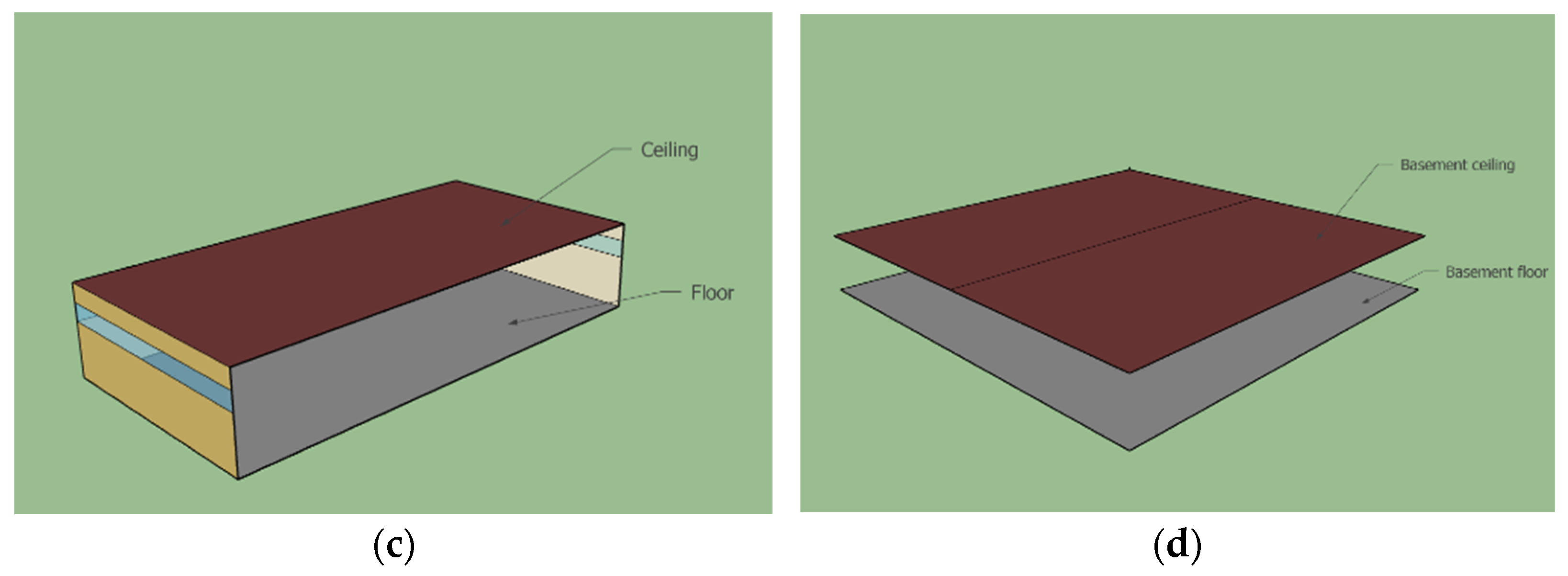
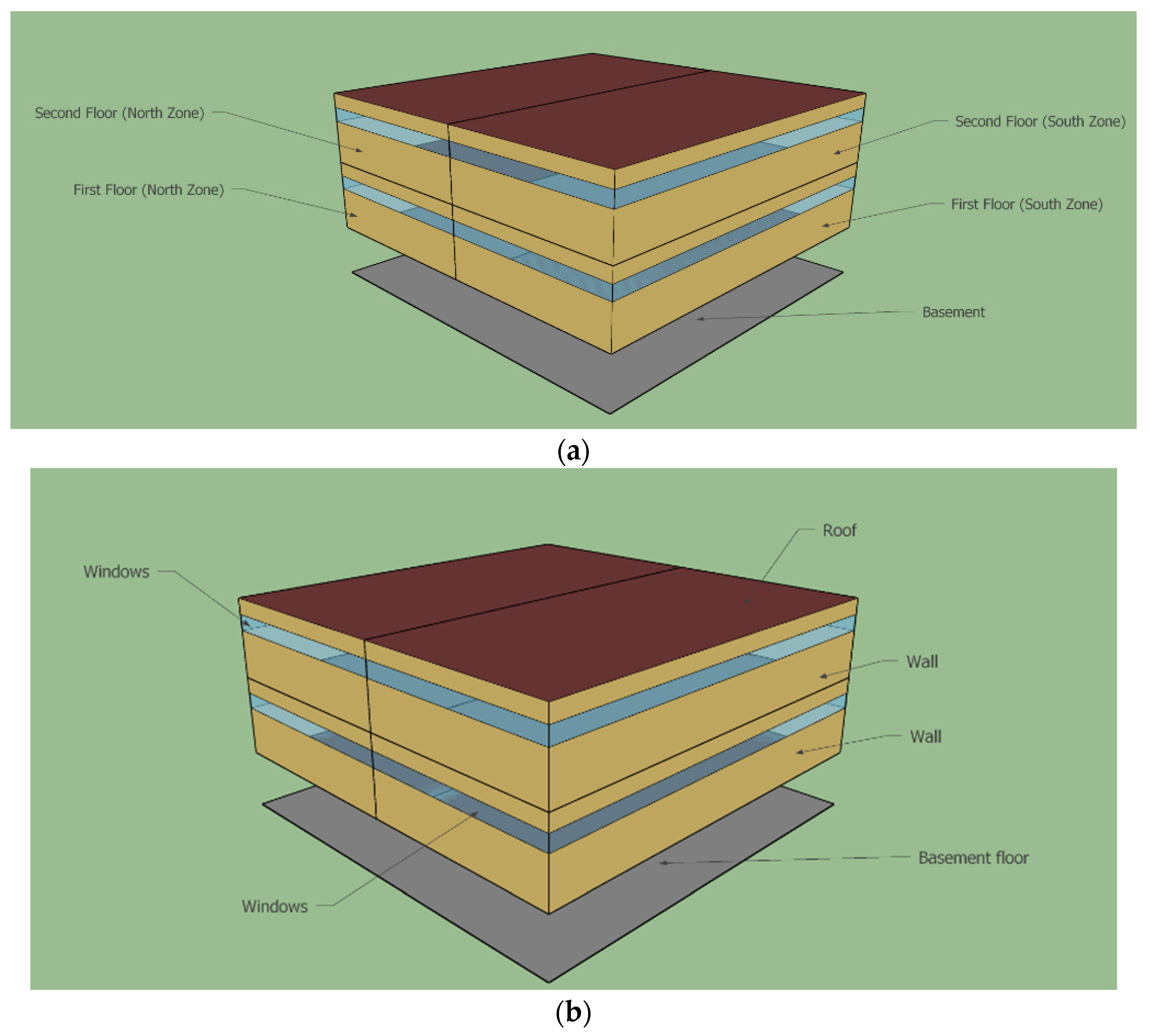
2.1. Building Description and Materials

The model of the building is an example obtained from an EnergyPlus Toolbox-GitHub repository [42] in order to avoid complex building configuration and focus on MPC control implementation. The building consists of two floors with similar geometry and a basement, as shown in Figure 1. Each floor has an area of 281.78 m², which is divided into a south and a north zone. There are two thermal zones per floor, corresponding to the north- and south-facing zones. Fixed windows run the length of each facade. The window-to-wall ratio (WWR) is 0.25. The glazing installed is a double-pane glass constituted by two clear glasses of 6 mm, a 6 mm space between, and a low-emissivity metallic coating on one pane surface. The walls are made of stone and gypsum board. They are insulated and have an air gap. The floor in both stories is ten centimeters of lightweight concrete, and it has carpet padding. The ceiling on the ground floor is made of ten centimeters of concrete and carpet padding, while on the second floor it is made of acoustic tile. The roof is built-up roofing with ten centimeters of concrete, insulation, and an air gap. The basement has the same ceiling construction as the ground floor, and the floor is fifteen centimeters of concrete.

Each thermal zone (the basement is unconditioned, but it has a heat source representing the equipment room) is served by a packaged single-zone (PSZ) HVAC system. Figure 2 shows a schematic diagram of the HVAC system for a single thermal zone. This configuration is also applied in the remaining thermal zones. The PSZ system has demand equipment and supply equipment. The demand equipment consists of a single duct, constant volume terminal unit without reheat coil (central air system) which regulates the volume of air to the occupied zone (ZNF1 thermal zone as shown in the figure). The supply equipment consists of a Direct Expansion (DX) cooling coil (single speed) for decreasing the temperature and pressure of the air passing through; a natural gas heating coil for increasing the temperature and pressure; and a draw to supply air fan (which means the fan is positioned downstream of the cooling coil) for circulating the air. Additionally, a setpoint manager for the thermal zone is shown in Figure 2, but this is not really a component of the HVAC system. Rather, this is a control construct of the simulation software that allows it to access data from the HVAC and use it for calculations.

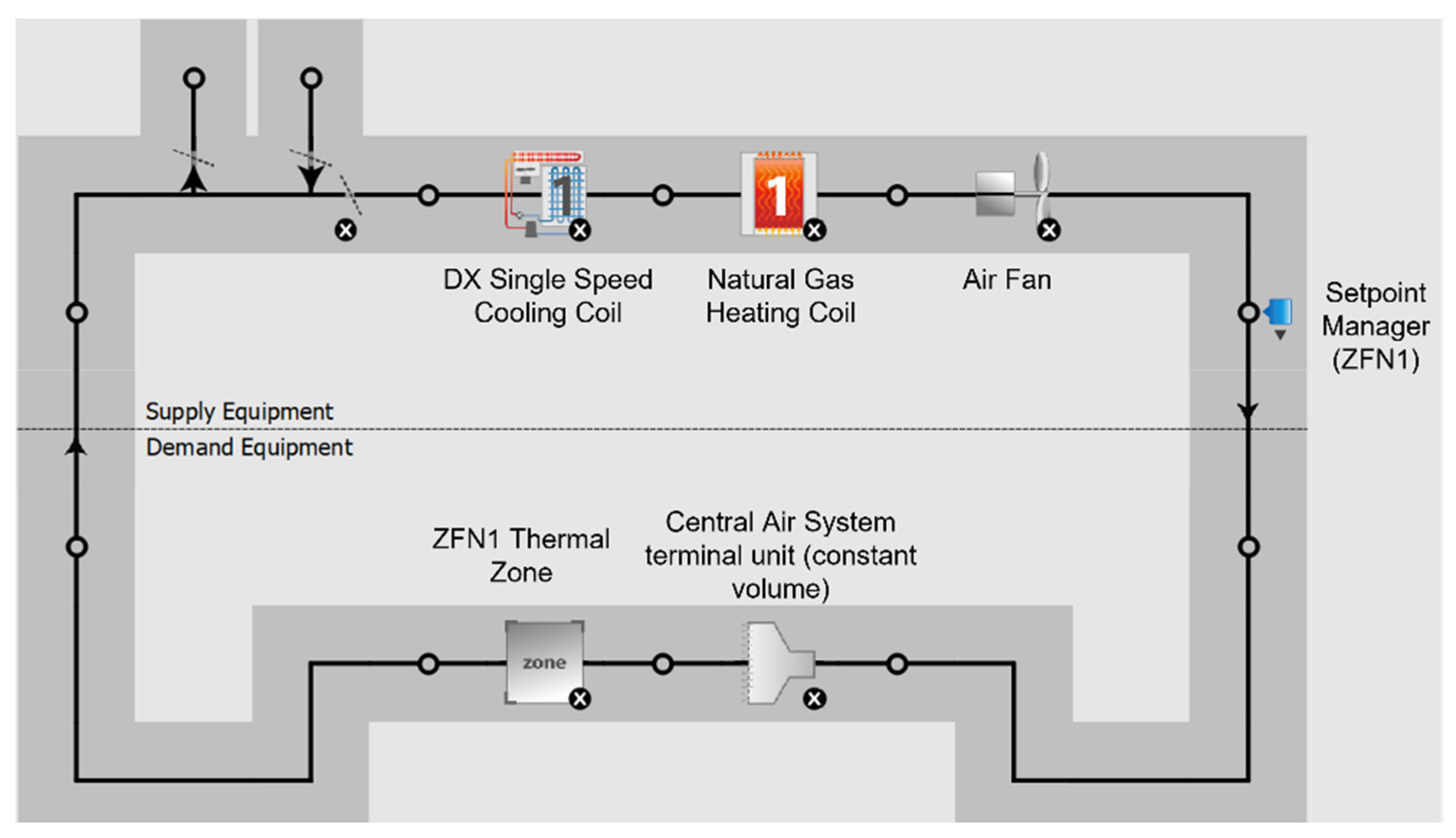
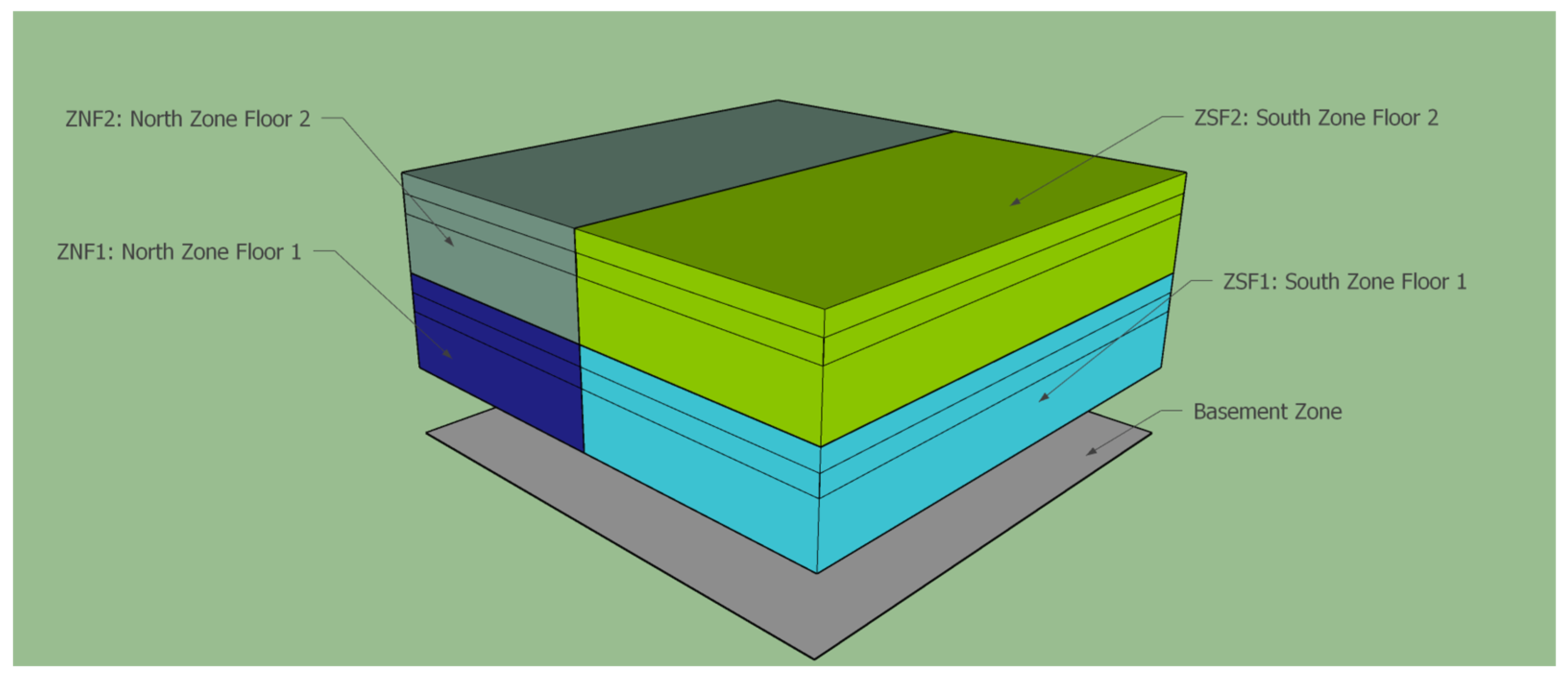
2.2. EnergyPlus Model

The building model and its HVAC system were developed with EnergyPlus. The building’s architecture and geometry are made with Google SketchUp, which is coupled to EnergyPlus using the Legacy Open Studio SketchUp plug-in. The FOMPC controller simulation scenario is applied to the north-facing thermal zone of floor 1 (the blue-colored zone in Figure 3), whose floor area is 154.70 m². Regarding the load configuration, lighting power is set to 3025 W, which implies an intensity of 19.55 watts/m². Electric equipment power is set to 687.5 W. There is one occupant per 47.3 m² of floor area (3.27 occupants in the zone). There is an internal mass occupying 77 m² (about half the floor area), which is made of 1.27 cm of wood. The infiltration design flow rate is 0.043 m³/s. There is a thermostat with a single heating or cooling setpoint related to the thermal zone and the HVAC system. The simulation run period is set from 1 to 30 June. This parameter is related to the meteorological data considered for EnergyPlus calculations.

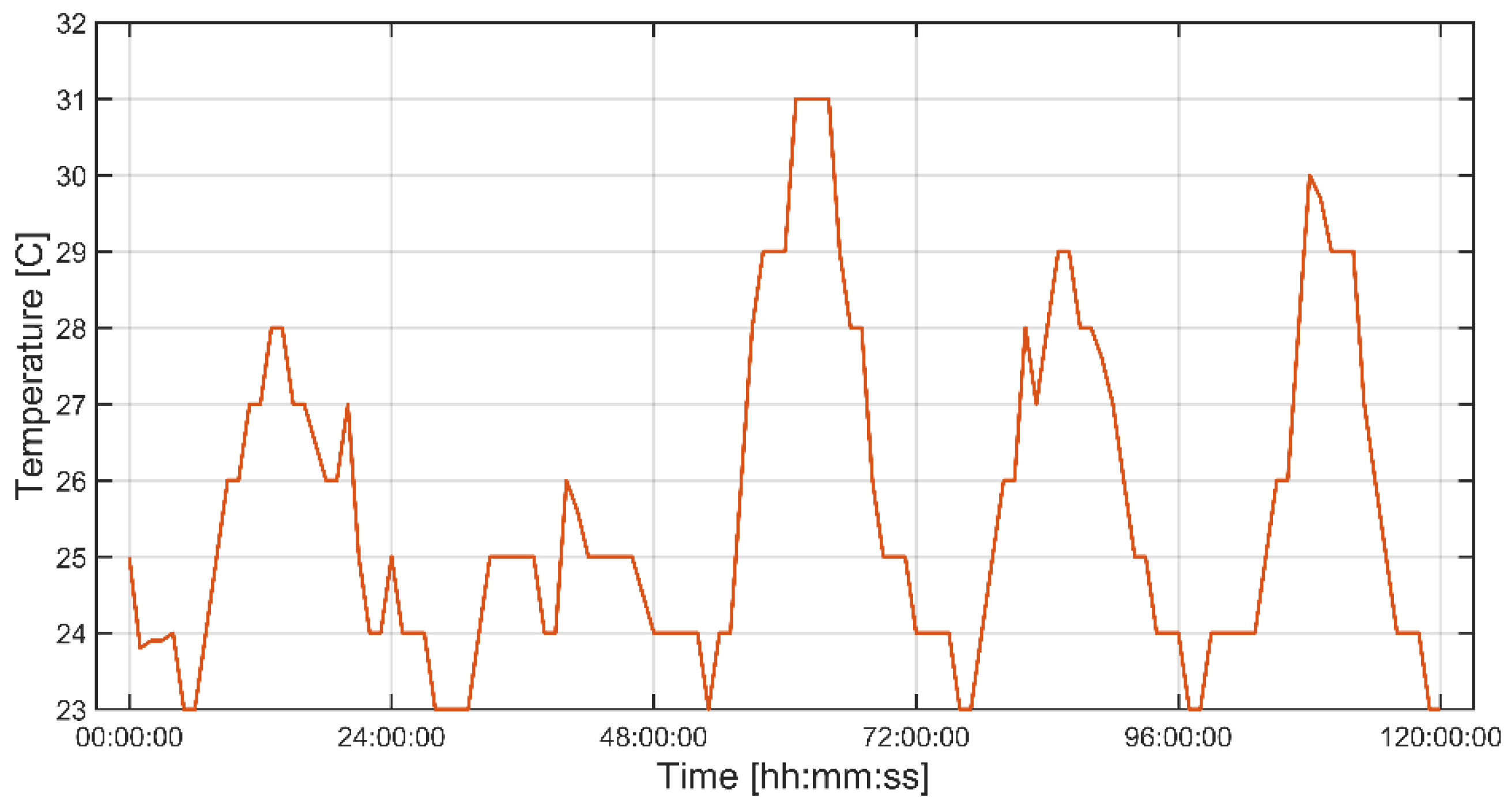
2.3. Meteorological Data

The weather data needed for the EnergyPlus calculations has been obtained as a licensed file from the ASHRAE Handbook [43]. The meteorological station is located at Jose Joaquin de Olmedo International Airport, located in Guayaquil, Ecuador. The main parameters of the file (also used for EnergyPlus calculations) are: dry bulb temperature (°C), dew point temperature (°C), relative humidity (%), atmospheric station pressure (Pa), horizontal infrared radiation intensity (Wh/m²), direct normal radiation (Wh/m²), diffuse horizontal radiation (Wh/m²), wind direction (°), wind speed (m/s) [44]. The weather data is TMY data, which means it is composed of 12 months of data, each chosen as the most typical among the total years. For this case, there is a range of data from 1990 to 2014 [45]. The data is also measured with an hourly time-step except for direct normal and diffuse radiation. Finally, the weather data for the outside air temperature (dry bulb temperature) for the city of Guayaquil through the first five days of the run period is shown in Figure 4.

2.4. System Identification

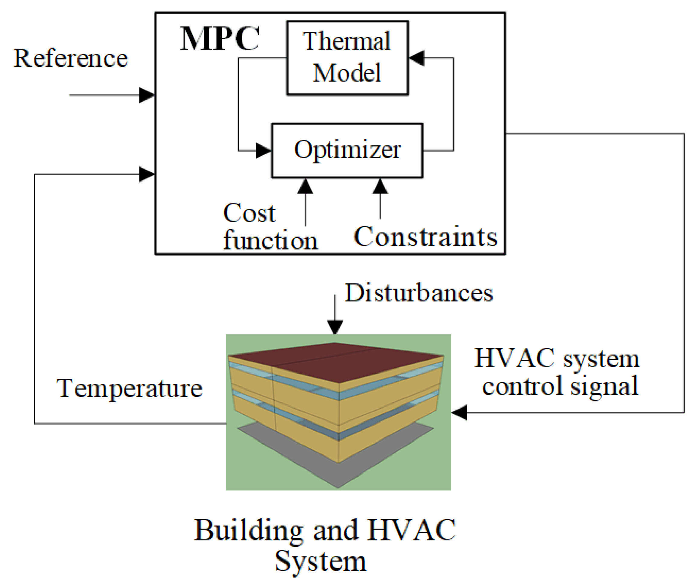
To design advanced model-based controllers, it is important to take into consideration the quality and accuracy of the model to be used, which is directly related to performance in terms of controller response. In addition, through the system model, the process characteristics can be simulated to avoid any damage in the equipment during the optimization process of the control method. Furthermore, since the temperature is a slow changing variable [39], a simple model may capture the dynamics of the system. Hence, we opted for a black-box model. In this regard, to get the input-output data, we run the EnergyPlus model using a Pseudo-Random Binary Signal (PRBS) [46] as the input signal $u\left(t\right)$ applied to north-faced thermal zone of floor 1 to get the temperature as the output signal $y\left(t\right)$. The following model has been obtained using Prediction Error Method (PEM):

$$G(s)=\frac{Y(s)}{U(s)}=\frac{0.85}{170.9s+1}{e}^{-46.9s}$$

(1)

where, $Y(s)=\mathcal{L}[y(t)]$ and $U(s)=\mathcal{L}[u(t)]$ are the Laplace transformations of $y(t)$ and $u(t)$, respectively.

3. Control Strategy

The predictive control strategy utilized hereafter is the Extended Prediction Self-Adaptive Control (EPSAC) formulation, whose basic structure is visualized in the block diagram of Figure 5. More information about this control method can be found in [47,48,49].

The process can be represented as:

$$y(t)=x(t)+w(t)$$

(2)

where, t is the discrete-time index, $y(t)$ is the process output, $x(t)$ is the model output and $w(t)$ represents the disturbances. The model output $x(t)$ depends on the past inputs and outputs.

$$y(t)=f[x(t-1),x(t-2),...,u(t-1),u(t-2),..]$$

(3)

The future input is obtained as follows:

$$u(t+k|t)=u_{base}(t+k|t)+\delta u(t+k|t)$$

(4)

where, $u_{base}(t+k|t)$ represents the basic future control actions and, $\delta u(t+k|t)$ is the cumulative effect of a series of impulse inputs and a step input and is the optimized future control actions. Based on these future input effects, the predicted system outputs can be defined as:

$$y(t+k|t)=y_{base}(t+k|t)+y_{opt}(t+k|t)$$

(5)

where, $y_{base}(t+k|t)$ is obtained by the basic future control action $u_{base}(t+k|t)$ and, $y_{opt}(t+k|t)$ is obtained with the optimized future control action $\delta u(t+k|t)$.

The $y_{opt}(t+k|t)$ is calculated according to:

$$y_{opt}(t+k|t)=h_k\delta u(t|t)+h_{k-1}\delta u(t+1|t)+...+g_{k-N_c+1}\delta u(t+N_c-1|t)$$

(6)

where, $N_c$ is the control horizon and $h_i$, $g_i$ are the coefficients of the impulse and step responses, respectively. The system output can be represented using matrix notation as follows:

$$Y=\overline{Y}+GU$$

(7)

where, $Y={[y(t+N_1|t)\cdots y(t+N_p|t)]}^T$, $U={[\delta u(t|t)\cdots \delta u(t+N_c-1|t)]}^T$, $\overline{Y}={[y_{base}(t+N_1|t)\cdots y_{base}(t+N_p|t)]}^T$, $N_1$ is the time delay of the system, $N_p$ is the prediction horizon and

$$G=\left[\begin{array}{llll}{h}_{N_1}& h_{N_1-1}& \cdots & g_{N_1-N_c+1}\\ h_{N_1+1}& h_{N_1}& \cdots & g_{N_2-N_c+1}\\ ⋮& ⋮& \ddots & ⋮\\ h_{N_p}& h_{N_p-1}& \cdots & g_{N_p-N_c+1}\end{array}\right]$$

The effects of the disturbances process output are considered in the term $w(t)$. It can be modeled using a colored noise process [48] as follows:

$$w(t+k|t)=\frac{C(q^{-1})}{D(q^{-1})}{w}_f(t+k|t)$$

(8)

where, $q^{-1}$ is the backward shift operator and $C(q^{-1})/D(q^{-1})$ is the disturbance model. Usually, a default disturbance model equal to an integrator is chosen $\frac{C(q^{-1})}{D(q^{-1})}=\frac{1}{1-q^{-1}}$ ensuring zero steady-state tracking-error [48].

The control signalis formulated by minimizing the following cost function:

$$J_{MPC}={\displaystyle \sum _{k=N_1}^{N_p}{\phi }_k{[r(t+k|t)-y(t+k|t)]}^2}+{\displaystyle \sum _{k=1}^{N_u}{\varphi }_k\Delta u{(t+k)}^2}$$

(9)

where $r(t+k|t)$ is the reference trajectory, and ${\phi }_k$ and ${\varphi }_k$ are nonnegative weighting factors, which are kept as constants.

Equation (9) can be expressed into matrix form as follows:

$${\mathrm{J}}_{\mathrm{MPC}}={(R-Y)}^T\Psi (R-Y)+U^T\Phi U={(R-\overline{Y}-GU)}^T\Psi (R-\overline{Y}-GU)+U^T\Phi U$$

(10)

where, $R={[r(t+N_1|t)\cdots r(t+N_p|t)]}^T$, $\Psi =diag({\phi }_1,{\phi }_2,...,{\phi }_{(N_p-N_1+1)})$ and $\Phi =diag({\varphi }_1,{\varphi }_2,...,{\varphi }_{N_u})$.

For processes with constraints, the mathematical optimization problem can be solved with quadratic programming (QP). Otherwise, the optimal sequence input $\delta u(t+k|t)$ is obtained as follows:

$$U_{\mathrm{MPC}}^{*}={(G^T\Psi G+\Phi )}^{-1}{G}^T\Psi (R-\overline{Y})$$

(11)

The Fractional-Order Model Predictive Control (FOMPC) formulation results from the generalization of the cost function (10) based on the fractional-order operator ${}^{\alpha }I{}_a^b(\cdot )$ [49], where $\mathit{\alpha }$ is the fractional order of integration in the [a, b] interval.

$$J_{FOMPC}={}^{\alpha }I_{N_1}^{N_p}{\phi }_k{[r(t+k|t)-y(t+k|t)]}^2+{}^{\beta }I{}_1^{Nu}{\varphi }_k\Delta u{(t+k)}^2$$

(12)

The cost function can be discretized with a sampling period $T_s$ and its representation into matrix form is given by:

$$J_{FOMPC}={(R-\overline{Y}-GU)}^T\Psi \Gamma (\alpha ,T_s)(R-\overline{Y}-GU)+U^T\Phi \Lambda (\beta ,T_s)U$$

(13)

where, $\Gamma$ and $\Lambda$ are weighting matrices obtained by the numerical evaluation of the fractional-order operators ${}^{\alpha }I_a^b(\cdot )$ and ${}^{\beta }I_a^b(\cdot )$ based on the Grunwald—Letnikov definition [50], which depends on the fractional terms $\alpha$ and $\beta$.

$$\Gamma (\alpha ,T_s)=T_s^{\alpha }diag(m_{N_p-N_1},m_{N_p-N_1-1},\cdots ,m_{1,}{m}_0)$$

(14)

$$\Lambda (\beta ,T_s)=T_s^{\beta }diag(m_{N_u},m_{N_u-1},\cdots ,m_1,m_0)$$

(15)

The $m_i$ terms with fractional order α or $\beta$ can be calculated as:

$$m_i={𝓁}_j^{(-\alpha )}-{𝓁}_{j-n}^{(-\alpha )}$$

(16)

where, $n$ is the number of the $m_i$ and $𝓁$ can be obtained with:

$${𝓁}_j^{(-\alpha )}=\left\{\begin{array}{ll}(1-(1-\alpha )/j){\omega }_{j-1}^{(-\alpha )}& j>0;\\ 1& j=0;\\ 0& j<0.\end{array}\right.$$

(17)

Similarly, this mathematical optimization problem can be solved with Quadratic programming (QP), when constraints for the system are considered. Otherwise, without constraints, the optimal sequence input $\delta u(t+k|t)$ is obtained as follows:

$$U_{\mathrm{FOMPC}}^{*}={(G^T\Psi (\Gamma +{\Gamma }^T)G+\Phi (\Lambda +{\Lambda }^T))}^{-1}{G}^T\Psi (\Gamma +{\Gamma }^T)(R-\overline{Y})$$

(18)

On the other hand, it is important to notice that the equivalent weighting factors for the FOMPC cost function result from the product $\Psi \Gamma (\alpha ,T_s)$ and $\Phi \Lambda (\beta ,T_s)$ for control increments and predicted error, respectively.

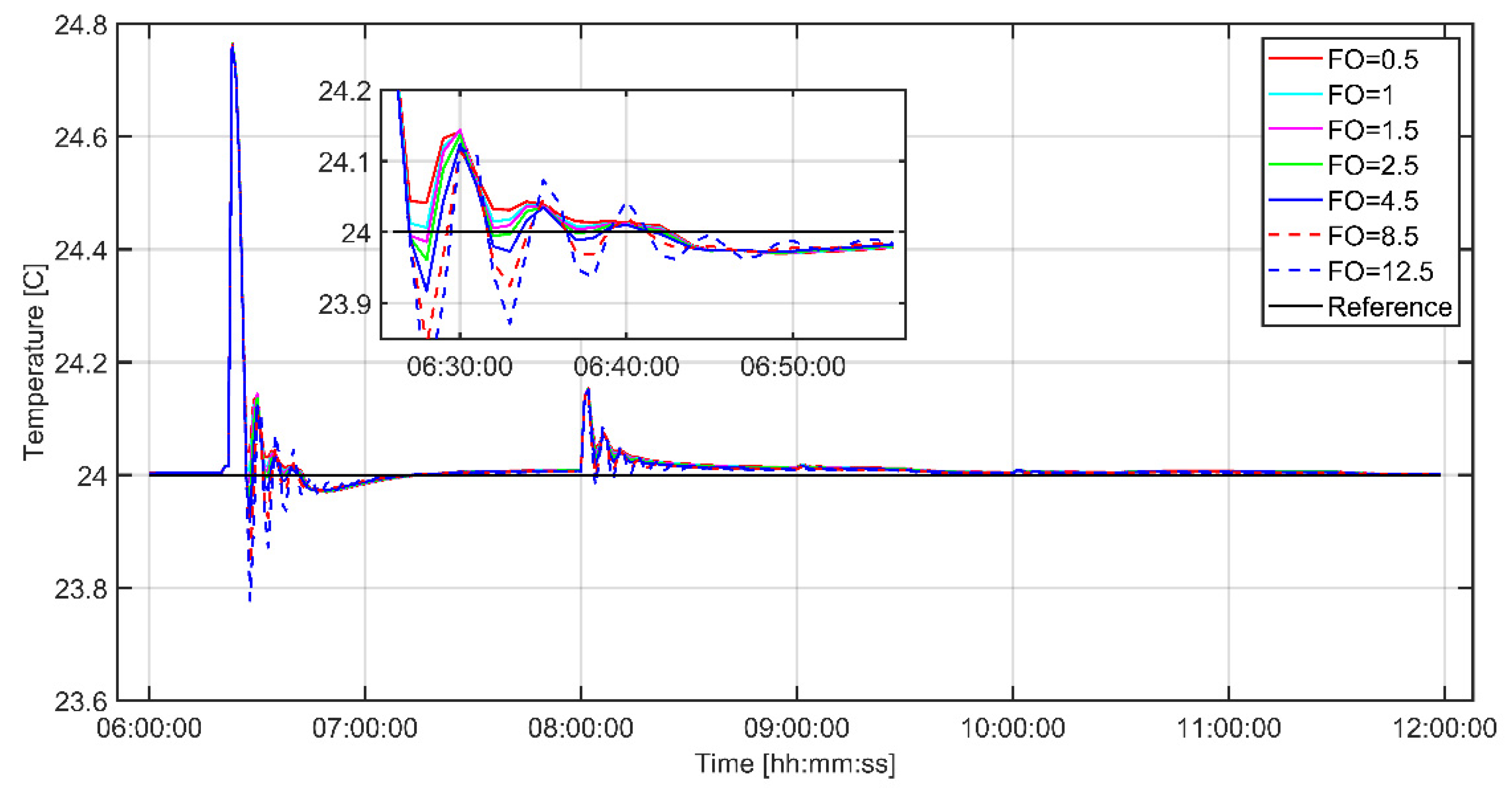
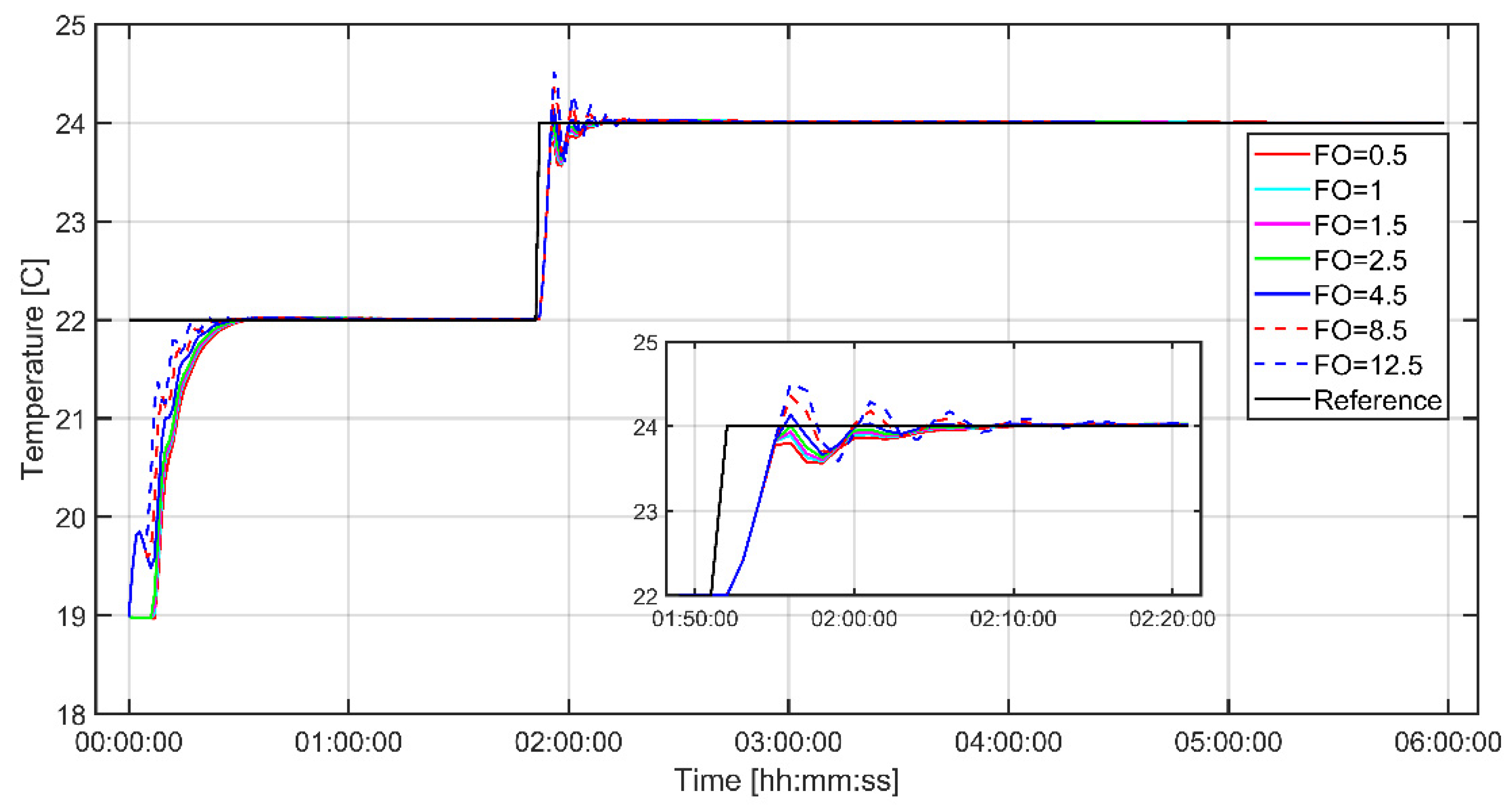
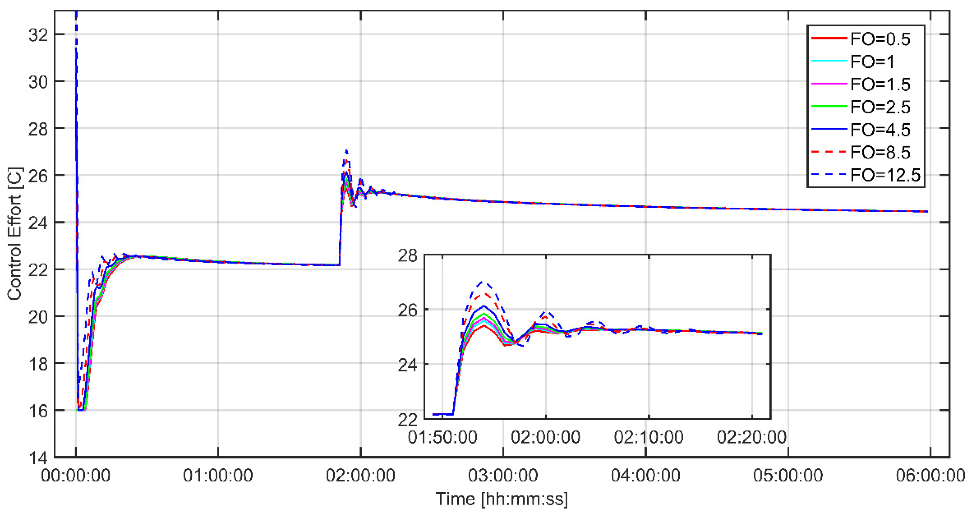
4. Results and Discussion

In this section, the results of the co-simulation between EnergyPlus and Matlab/Simulink for a building energy management system focused on thermal zone control are presented. Hence, the reference tracking and disturbance rejection experiments are conducted to verify the performance of the proposed FOMPC algorithm.

Parameters N1, Np, and Nu are chosen following the thumb-rules [51], and a default disturbance model has been selected as an integrator to guarantee zero steady-state error. These parameters are summarized in

Table 1. MPC parameters.

Parameters	Nu	Np	Ts	N1
Values	1	30	60 s	1

.

The weights of the objective function (see Equation (12)) are directly related to the optimal closed-loop response, $\alpha$ for the reference tracking and $\beta$ for the control signal. Therefore, it is important to study the influence of these parameters on the performance of the proposed control system proposed. In this study, $\alpha$ and $\beta$ are chosen to be the same for simplification. The results for different fractional order (FO) terms are depicted in Figure 6 and Figure 7.

From the results shown in Figure 6, we can see the effect of the fractional terms on the settling time, overshoot, and control effort of the system, which indicate that for a certain range of values of the fractional order, better responses are obtained both in settling time and overshoot when considering the reference tracking. However, we cannot simply use this result of reference tracking to select the more appropriate controller. Furthermore, it is important to analyze the control effort (see Figure 7) in order to select the best fractional order value to have a trade-off between tracking and control effort. Note that when the fraction terms are equal to 1, we have the case of a classical MPC.

On the other hand, Figure 8 depicts the disturbance rejection performance of the controller for different fractional values. We can see that for fractional values between 2 < FO < 8 the performance of the controller has a better disturbance suppression ability with respect to the traditional MPC (FO = 1).

For a better analysis based on numerical results, the following performance measures are applied to evaluate the performance of the FOMPC and MPC (FO = 1), including the Integrated Absolute Error (IAE), Integral Secondary control output (ISU), Ratio of Integrated Absolute Relative Error (RIARE), and Ratio of Integral Secondary control output (RISU). These indexes allow for the evaluation of the performance of reference tracking, disturbance rejection, and energy use by the controller.

$$IAE={\displaystyle \sum _{k=0}^{N_s-1}\left|r(k)-y(k)\right|}; ISU={\displaystyle \sum _{k=0}^{N_s-1}{\left(u(k)-u_{ss}(k)\right)}^2}$$

(19)

$$RIAE(C_2,C_1)=\frac{IAE(C_2)}{IAE(C_1)}; RISU(C_2,C_1)=\frac{ISU(C_2)}{ISU(C_1)}$$

(20)

where, $N_s$ is the number of simulation steps, $u_{ss}$ is the steady state value of the control effort and $C_1$, $C_2$ are the two compared controllers ((MPC is C₂ and FOMPC is C₁).

The results of this evaluation with different fractional terms are shown in

Table 2. Performance indexes for reference tracking and control effort.

Index	FO (0.5)	FO (1)	FO (1.5)	FO (2)	FO (2.5)	FO (3)	FO (4)	FO (4.5)
IAE	9.0898	8.5755	8.3136	8.1064	7.9328	7.8286	7.7099	7.6835
ISU	32.9162	33.8012	34.4025	34.9530	35.5080	36.0807	37.2308	37.8603
RIAE	0.9434	1	1.0315	1.0579	1.0810	1.0954	1.1123	1.1161
RISU	1.0269	1	0.9825	0.9670	0.9519	0.9368	0.9079	0.8928

and

Table 3. Performance indexes for reference tracking and control effort.

Index	FO (5)	FO (6)	FO (7)	FO (8)	FO (8.5)	FO (9)	FO (10)	FO (12.5)
IAE	7.6667	7.6849	7.7938	8.0320	8.1662	8.3047	8.6038	9.1152
ISU	38.5106	39.8635	41.2617	42.7213	43.4871	44.2778	45.9401	50.1256
RIAE	1.1185	1.1159	1.1003	1.0677	1.0501	1.0326	0.9967	0.9408
RISU	0.8777	0.8479	0.8192	0.7912	0.7773	0.7634	0.7358	0.6743

.

The results presented in Table 2 and Table 3 indicate that for fractional order values between 2 < FO < 8, a better controller performance is achieved during trajectory tracking (IAE index). Something similar happens with the control effort (ISU index): for a fractional range of values, less energy consumption is obtained compared to the MPC. Therefore, a trade-off between tracking and the control effort is achieved with FO = 2.5. This conclusion can also be drawn according to the RIAE and RISU indexes.

5. Conclusions

We have designed an FOMPC for the temperature control of a thermal zone of a building. As the capacity to process data is increasing, several sensors can monitor different variables of a building, and we can represent a model in specialized software like EnergyPlus. Additionally, an extensive analysis of the effect of the fractional weighting sequences on the FOMPC performance is presented. Therefore, it is only necessary to optimize the fractional orders $(\alpha ,\beta )$, to automatically generate non-constant weighting sequences that allow us to modify the final weighting factors $\Psi \Gamma (\alpha ,T_s)$ and $\Phi \Lambda (\beta ,T_s)$ considering the cost function. Here, these terms are considered high-level parameters to construct non-constant weighting sequences, which can have negative elements when the fractional terms are less than 1. The results demonstrate the advantage of the fractional controller during the temperature control of a thermal zone and an improvement in disturbance rejection due to external temperature changes to which the building is subjected. Undoubtedly, the achieved improvement is due to the inherent characteristics of the fractional terms in the FOMPC algorithm.

A further step is to apply the developed technique in a real-world setting. First, a building model should be constructed in EnergyPlus. Second, the model should be validated from measured data through several tests. Third, with a validated model, we can identify the model. Furthermore, we can design an MPC controller with fractional order weights until the objectives are met. Finally, the control is applied, tested, and redesigned if necessary.

References

1. González-Torres, M.; Pérez-Lombard, L.; Coronel, J.F.; Maestre, I.R.; Yan, D. A review on buildings energy information: Trends, end-uses, fuels and drivers. Energy Rep. 2022, 8, 626–637. [Google Scholar] [CrossRef]
2. 2019 Global Status Report for Buildings and Construction Sector. Available online: https://www.unep.org/resources/publication/2019-global-status-report-buildings-and-construction-sector (accessed on 29 July 2022).
3. Sources of Greenhouse Gas Emissions. Available online: https://www.epa.gov/ghgemissions/sources-greenhouse-gas-emissions#commercial-and-residential (accessed on 29 July 2022).
4. Royapoor, M.; Antony, A.; Roskilly, T. A review of building climate and plant controls, and a survey of industry perspectives. Energy Build. 2018, 158, 453–465. [Google Scholar] [CrossRef]
5. Ma, Y.; Borrelli, F.; Hencey, B.; Coffey, B.; Bengea, S.; Haves, P. Model predictive control for the operation of building cooling systems. IEEE Trans. Control. Syst. Technol. 2012, 20, 796–803. [Google Scholar]
6. Kathirgamanathan, A.; De Rosa, M.; Mangina, E.; Finn, D.P. Data-driven predictive control for unlocking building energy flexibility: A review. Renew. Sustain. Energy Rev. 2021, 135, 110120. [Google Scholar] [CrossRef]
7. Carlet, P.G.; Favato, A.; Bolognani, S.; Dörfler, F. Data-driven continuous-set predictive current control for synchronous motor drives. IEEE Trans. Power Electron. 2022, 37, 6637–6646. [Google Scholar] [CrossRef]
8. Zhang, X.; Cheng, Y.; Zhang, L. Disturbance-deadbeat inductance observer-based current predictive control for surface-mounted permanent magnet synchronous motors drives. IET Power Electron. 2020, 13, 1172–1180. [Google Scholar] [CrossRef]
9. Jiang, X.; Yang, Y.; Fan, M.; Ji, A.; Xiao, Y.; Zhang, X.; Zhang, W.; Garcia, C.; Vasquez, S.; Rodriguez, J. An improved implicit model predictive current control with continuous control set for PMSM drives. IEEE Trans. Transp. Electrif. 2022, 8, 2444–2455. [Google Scholar] [CrossRef]
10. Abu-Ali, M.; Berkel, F.; Manderla, M.; Reimann, S.; Kennel, R.; Abdelrahem, M. Deep learning-based long-horizon MPC: Robust, high performing and computationally efficient control for PMSM drives. IEEE Trans. Power Electron. 2022, 37, 12486–12501. [Google Scholar] [CrossRef]
11. Zhao, S.; Cajo, R.; De Keyser, R.; Ionescu, C.M. The potential of fractional order distributed MPC applied to steam/water loop in large scale ships. Processes 2020, 8, 451. [Google Scholar] [CrossRef]
12. Zhao, S.; Cajo, R.; De Keyser, R.; Liu, S.; Ionescu, C.M. Nonlinear predictive control applied to steam/water loop in large scale ships. IFAC Pap. 2019, 52, 868–873. [Google Scholar] [CrossRef]
13. Cheng, C.; Peng, C.; Zhang, T. Fuzzy k-means cluster based generalized predictive control of ultra supercritical power plant. IEEE Trans. Ind. Inform. 2021, 17, 4575–4583. [Google Scholar] [CrossRef]
14. Bonfiglio, A.; Cantoni, F.; Oliveri, A.; Procopio, R.; Rosini, A.; Invernizzi, M.; Storace, M. An MPC-based approach for emergency control ensuring transient stability in power grids with steam plants. IEEE Trans. Ind. Electron. 2019, 66, 5412–5422. [Google Scholar] [CrossRef]
15. Yang, S.; Wan, M.P.; Chen, W.; Ng, B.F.; Dubey, S. Experiment study of machine-learning-based approximate model predictive control for energy-efficient building control. Appl. Energy 2021, 288, 116648. [Google Scholar] [CrossRef]
16. Yang, S.; Wan, M.P.; Chen, W.; Ng, B.F.; Dubey, S. Model predictive control with adaptive machine-learning-based model for building energy efficiency and comfort optimization. Appl. Energy 2020, 271, 115147. [Google Scholar] [CrossRef]
17. Rout, R.; Subudhi, B. Design of line-of-sight guidance law and a constrained optimal controller for an autonomous underwater vehicle. IEEE Trans. Circuits Syst. II Express Briefs 2021, 68, 416–420. [Google Scholar] [CrossRef]
18. Heshmati-Alamdari, S.; Karras, G.C.; Marantos, P.; Kyriakopoulos, K.J. A robust predictive control approach for underwater robotic vehicles. IEEE Trans. Control Syst. Technol. 2020, 28, 2352–2363. [Google Scholar] [CrossRef]
19. Afram, A.; Janabi-Sharifi, F. Theory and applications of HVAC control systems—A review of model predictive control (MPC). Build. Environ. 2014, 72, 343–355. [Google Scholar]
20. Taheri, S.; Hosseini, P.; Razban, A. Model predictive control of heating, ventilation, and air conditioning (HVAC) systems: A state-of-the-art review. J. Build. Eng. 2022, 60, 105067. [Google Scholar] [CrossRef]
21. Dastjerdi, A.A.; Vinagre, B.M.; Chen, Y.; HosseinNia, S.H. Linear fractional order controllers; A survey in the frequency domain. Annu. Rev. Control 2019, 47, 51–70. [Google Scholar] [CrossRef]
22. Moreles, M.; Lainez, R. Mathematical modelling of fractional order circuit elements and bioimpedance applications. Commun. Nonlinear Sci. Numer. Simul. 2017, 46, 81–88. [Google Scholar] [CrossRef]
23. Zheng, W.; Huang, R.; Luo, Y.; Chen, Y.; Wang, X.; Chen, Y. A look-up table based fractional order composite controller synthesis method for the pmsm speed servo system. Fractal Fract. 2022, 6, 47. [Google Scholar] [CrossRef]
24. Cajo, R.; Mac, T.T.; Plaza, D.; Copot, C.; De Keyser, R.; Ionescu, C. A survey on fractional order control techniques for unmanned aerial and ground vehicles. IEEE Access 2019, 7, 66864–66878. [Google Scholar] [CrossRef]
25. Hashemizadeh, E.; Ebrahimzadeh, A.; Physica, A. An efficient numerical scheme to solve fractional diffusion-wave and fractional Klein-Gordon equations in fluid mechanics. Stat. Mech. Its Appl. 2018, 503, 1189–1203. [Google Scholar] [CrossRef]
26. Yang, F.; Mou, J.; Liu, J.; Ma, C.; Yan, H. Characteristic analysis of the fractional-order hyperchaotic complex system and its image encryption application. Signal Process. 2020, 169, 107373. [Google Scholar] [CrossRef]
27. Sohail, A.; Beg, O.; Li, Z.; Celik, S. Physics of fractional imaging in biomedicine. Prog. Biophys. Mol. Biol. 2018, 140, 13–20. [Google Scholar] [CrossRef]
28. Ivanescu, M.; Dumitrache, I.; Popescu, N.; Popescu, D. Fractional order model identification of a person with Parkinson’s disease for wheelchair control. Fractal Fract. 2023, 7, 23. [Google Scholar] [CrossRef]
29. Huang, C.; Wang, J.; Chen, X.; Cao, J. Bifurcations in a fractional-order BAM neural network with four different delays. Neural Netw. 2021, 141, 344–354. [Google Scholar] [CrossRef]
30. Huang, C.; Liu, H.; Shi, X.; Chen, X.; Xiao, M.; Wang, Z.; Cao, J. Bifurcations in a fractional-order neural network with multiple leakage delays. Neural Netw. 2020, 131, 115–126. [Google Scholar] [CrossRef]
31. Li, P.; Li, Y.; Gao, R.; Xu, C.; Shang, Y. New exploration on bifurcation in fractional-order genetic regulatory networks incorporating both type delays. Eur. Phys. J. Plus 2022, 137, 598. [Google Scholar] [CrossRef]
32. Afram, A.; Janabi-Sharifi, F. Review of modeling methods for HVAC systems. Appl. Therm. Eng. 2014, 67, 507–519. [Google Scholar] [CrossRef]
33. Zhan, S.; Chong, A. Data requirements and performance evaluation of model predictive control in buildings: A modeling perspective. Renew. Sustain. Energy Rev. 2021, 142, 110835. [Google Scholar] [CrossRef]
34. Kim, D.; Lee, J.; Do, S.; Mago, P.J.; Lee, K.H.; Cho, H. Energy Modeling and Model Predictive Control for HVAC in Buildings: A Review of Current Research Trends. Energies 2022, 15, 7231. [Google Scholar] [CrossRef]
35. Afram, A.; Janabi-Sharifi, F. Gray-box modeling and validation of residential HVAC system for control system design. Appl. Energy 2015, 137, 134–150. [Google Scholar] [CrossRef]
36. Crawley, D.B.; Lawrie, L.K.; Winkelmann, F.C.; Buhl, W.F.; Huang, Y.J.; Pedersen, C.O.; Strand, R.K.; Liesen, R.J.; Fisher, D.E.; Witte, M.J.; et al. EnergyPlus: Creating a new-generation building energy simulation program. Energy Build. 2001, 33, 319–331. [Google Scholar] [CrossRef]
37. Klein, S.A.; Beckman, W.A.; Mitchell, J.W.; Duffie, J.A.; Duffie, N.A.; Freeman, T.L.; Mitchell, J.C.; Braun, J.E.; Evans, B.L.; Kummer, J.P.; et al. TRNSYS 17: A Transient System Simulation Program, Solar Energy Laboratory; University of Wisconsin: Madison, WI, USA, 2010. [Google Scholar]
38. Ferrarini, L.; Fathi, E.; Disegna, S.; Rastegarpour, S. Energy consumption models for residential buildings: A case study. In Proceedings of the 2019 24th IEEE International Conference on Emerging Technologies and Factory Automation (ETFA), Zaragoza, Spain, 10–13 September 2019. [Google Scholar]
39. Široký, J.; Oldewurtel, F.; Cigler, J.; Prívara, S. Experimental analysis of model predictive control for an energy efficient building heating system. Appl. Energy 2011, 88, 3079–3087. [Google Scholar] [CrossRef]
40. Martinčević, A.; Vašak, M. Constrained Kalman filter for identification of semiphysical building thermal models. IEEE Trans. Control Syst. Technol. 2020, 28, 2697–2704. [Google Scholar] [CrossRef]
41. Zhao, S.; Wang, S.; Cajo, R.; Ren, W.; Li, B. Power tracking control of marine boiler-turbine system based on fractional order model predictive control algorithm. J. Mar. Sci. Eng. 2022, 10, 1307. [Google Scholar] [CrossRef]
42. dostaji4/EnergyPlus-Co-Simulation-Toolbox. Available online: https://github.com/dostaji4/EnergyPlus-co-simulation-toolbox (accessed on 5 May 2022).
43. ASHRAE Handbook. Available online: https://www.ashrae.org/technical-resources/ashrae-handbook (accessed on 1 September 2022).
44. Climate.OneBuilding.Org. Available online: https://climate.onebuilding.org/papers/EnergyPlus_Weather_File_Format.pdf (accessed on 5 May 2022).
45. Ebrahimpour, A. New Software for Generation of Typical Meteorological Year. In Proceedings of the World Renewable Energy Congress, Linköping, Sweden, 8–13 May 2011. [Google Scholar]
46. Ljung, L. System Identification Toolbox for Use With Matlab, 6th ed.; The Math-Works: Natick, MA, USA, 2003. [Google Scholar]
47. De Keyser, R. Model based predictive control for linear systems. In Control Systems, Robotics and Automation, Advanced Control Systems V; Unbehauen, H., Ed.; EOLSS Publishers/UNESCO: Oxford, UK, 2003; Volume XI, pp. 24–58. [Google Scholar]
48. De Keyser, R.; Ionescu, C.M. The disturbance model in model based predictive control. In Proceedings of the 2003 IEEE Conference on Control Applications, 2003 (CCA 2003), Istanbul, Turkey, 25 June 2003. [Google Scholar]
49. Fernandez, E.; Ipanaque, W.; Cajo, R.; De Keyser, R. Classical and advanced control methods applied to an anaerobic digestion reactor model. In Proceedings of the 2019 IEEE CHILEAN Conference on Electrical, Electronics Engineering, Information and Communication Technologies (CHILECON), Valparaiso, Chile, 13–27 November 2019. [Google Scholar]
50. Romero, M.; de Madrid, A.P.; Vinagre, B.M. Arbitrary real-order cost functions for signals and systems. Signal Process. 2011, 91, 372–378. [Google Scholar] [CrossRef]
51. Clarke, D.W.; Mohtadi, C.; Tuffs, P.S. Generalized predictive control—Part I. The basic algorithm. Automatica 1987, 23, 137–148. [Google Scholar] [CrossRef]
Figure 1. 3D View of the building design in Google Sketchup. (a) The north and south zones of each floor and the basement are labeled. (b) The walls, windows, roof, and basement floor are identified since they can be easily observed. (c) Shows the north zone of the first floor as a separate construction. As evidenced, there is no wall separating the north and south zones (this also applies to the second floor). Also, the ceiling and the floor are identified by labels. These elements can be similarly observed within the other zones, but on the second floor, there will be the roof rather than the ceiling. (d) Shows the basement, which is described by only two elements in this model: the floor and the ceiling.
Fractalfract 07 00172 g001aFractalfract 07 00172 g001b
Figure 2. HVAC loop for the air system established at the thermal zone under study. The HVAC loop is divided into two sub-loops: a demand loop and a supply loop. Each sub-loop comprises an inlet connection that is connected (following the direction of the arrows) via a number of components to an outlet connection. The supply loop is where the energy is supplied by the system; consequently, it incorporates specialized equipment as shown in the diagram (heating and cooling coils and an air fan). In the demand loop, the energy is extracted from the system so that it incorporates zone air distribution equipment (the air terminal unit shown in the diagram). Since the HVAC loop is constructed within Open-Studio, it includes a setpoint manager object at the supply loop section and a thermal zone object (labeled as ZFN1 Thermal Zone) at the demand loop section. The arrows in the diagram’s upper left corner represent an outdoor air mixer.
Fractalfract 07 00172 g002
Figure 3. Thermal zones defined in the building model. As previously stated in this article, there are two thermal zones per floor, and in the figure, each one is distinguished by a particular color (also by labels). The color-distinguished building model was obtained by applying the thermal zone rendering tool within the SketchUp-OpenStudio environment. The ZNF1 thermal zone is where the controller is applied.
Fractalfract 07 00172 g003
Figure 4. Outside air temperature for the city of Guayaquil. The hourly dry bulb temperature corresponding to the rows in the weather file from 1 to 5 June is depicted in this graph.
Fractalfract 07 00172 g004
Figure 5. The proposed scheme of MPC integrating a thermal model in EnergyPlus. The optimizer is composed of a quadratic objective function in the presence of constraints, which is solved by quadratic programming.
Fractalfract 07 00172 g005
Figure 6. Temperature control for thermal zone with different fractional order terms. FO = 1 represents the particular case of an integer order system (MPC).
Fractalfract 07 00172 g006
Figure 7. Control effort with different fractional order terms. FO = 1 represents the particular case of an integer order system (MPC).
Fractalfract 07 00172 g007
Figure 8. Disturbance rejection for thermal zone with different fractional order terms. FO = 1 represents the particular case of an integer order system (MPC).
Fractalfract 07 00172 g008