Nanoscale 3D Spatial Analysis of Zirconia Disc Surfaces Subjected to Different Laser Treatments

Abstract

We propose the application of morphological, fractal and multifractal analysis to differentiate surface patterns on zirconia-based ceramics after laser treatments. Furthermore, we introduce two new approaches for ceramic surfaces: the Moran correlogram, which complements the spatial autocorrelation analyses, and the Otsu binarization algorithm, which was used to identify the lacunar points in the lacunarity analysis. First, the AFM (Atomic Force Microscope) topographies revealed that samples have significant differences in terms of spatial features. Quantitatively, spatial surface texture parameters indicated that all laser treatments reduced the superficial isotropy of the Zirconia disc. Moran’s correlograms revealed a decrease in the short-range correlation in all treated samples. The Minkowski functionals (MFs) indicated a reduction in the amount of matter in the peaks, especially for the sample with Nd-YAG laser treatment. The estimated fractal dimension (FD) pointed out that all laser treatments weakened the surface complexity of the Zirconia disc. On the other hand, clear fingerprints of multifractal behavior in all the samples were detected, where the highest degree of multifractality was computed for the samples with CO₂ laser treatment. Finally, our findings suggested that the morphological changes caused by laser treatments on the surfaces of zirconia discs can be monitored and differentiated through the parameters proposed here.

1. Introduction

Zirconia-based ceramic has great potential for alternative material to titanium in dentistry, mainly due to its tooth-like color, biocompatibility and suitable mechanical properties [1,2,3,4]. In addition to the physical–chemical, mechanical and biological properties, the surface topography of the dental implants also plays an important role [4,5,6].

Some studies in the literature showed that implants made with modified zirconia have a much better osseointegration than those made with non-modified zirconia [7,8,9,10]. Actually, surface modification can improve adhesion and increase the clinical utility of zirconia restorations [11]. The most commonly used methods for modifying the surface of zirconia implants are machining [12], sandblasting [7], chemical etching [13], laser treatment [14] and coating [15]. However, laser processing has some advantages.

In laser treatment, generally, there is no surface contamination because it is a contact-free process [16]. Laser treatment can also produce hierarchical surface structures with regular patterns [5,6]. Such processing can still be applied to any kind of material [17]. Furthermore, laser treatment is considered one of the best methods to increase the service life of ceramic material [6]. In this context, some solid-state (e.g., Nd-YAG and Er-YAG lasers) and gas (e.g., CO₂ laser) lasers have been proposed to modify the surface characteristics of ceramics [6,18,19].

In dentistry, Er-YAG lasers are used for caries removal [20], Nd-YAG lasers are used in the treatment of tooth hypersensitivity, bleaching and reducing reinfection of root canals [18,19] and CO2 lasers are used in gingivectomy and excisional biopsies [21].

On the other hand, the multiscale spatial pattern of ZrO₂ can be influenced by surface treatment, enabling modifications that can generate improved surface characteristics [22,23]. However, as far as we know, there is no consensus in the literature regarding the most efficient approach to verify and differentiate changes in surface patterns caused by laser treatments.

For a long time, several studies have confirmed the efficiency of using fractal and multifractal analysis through AFM (Atomic Force Microscope) images for monitoring nanoscale surface patterns [24,25], including laser-modified polymeric surfaces [26] and biological surfaces [27,28]. Thus, our purpose in this work is to investigate the influence of treatment with Nd-YAG, Er-YAG and CO₂ lasers on the nanoscale surface patterns of Zirconia-based ceramic through morphological, fractal and multifractal analysis. Actually, we want to verify whether these analyses are efficient in differentiating surface patterns after laser treatments. Furthermore, we used Moran’s correlogram to complement the spatial autocorrelation analyses and the Otsu binarization algorithm to identify the lacunar points of the lacunarity analysis. Both approaches, as far as we know, are unpublished for evaluating patterns on ceramic surfaces.

2. Materials and Methods

2.1. Preparation of Zirconia Ceramic Discs

Zirconia (ZrO₂) ceramic discs (3 mm in thickness and 7 mm in diameter) were obtained by copy-milling technique (Zirkon Zahn GmbH, Bruneck, Italy) using a previous reported protocol [6]. According to that protocol, the obtained samples were annealed at 1500 °C and further polished using silicon carbide abrasive paper (English Abrasives, London, UK) by 600, 800 and 1200 grits. As an experiment control, one untreated single ZrO₂ disc was named S1. Subsequently, the ZrO₂ discs were irradiated by the Nd-YAG (duration time: 15 s; laser power: 20 W; beam energy: 200 mJ; number of repetitions: 10; laser wavelength: 2.94 µm; pulse width: 0.7 ms; beam distance: 10 mm; amplitude: 10%), Er-YAG (duration time: 20 s; laser power: 2 W; beam energy: 200 mJ; number of repetitions: 10; laser wavelength: 1.064 µm; pulse width: 0.3 ms; beam distance: 10 mm; amplitude: 10%) and CO₂ (duration time: 20 s; laser power: 3 W; beam energy: 300 mJ; number of repetitions: 100; laser wavelength: 10.16 µm; pulse width: 160 ms; beam distance: 10 mm; amplitude: 90%) lasers, which were labeled as S2, S3 and S4, respectively. The resultant samples were chilled at room temperature for further characterization.

We used Neodymium: Ytterbium Aluminum Garnet (Nd:YAG) nanosecond laser source (Q-PLUS model from Spectrum. A. T. N. Ltd., Toronto, ON, Canada), Erbium-yttrium Aluminum Garnet (Er: YAG) laser (Hoya model from Con Bio, Base Seattle, WA, USA) and Carbon Dioxide (CO₂) laser (LightScalpel LS-1005 CO₂, Base Seattle, WA, USA).

2.2. AFM Imaging

The 3D AFM topographical maps were accessed using a Nanoscope Multimode (Digital Instruments, Santa Barbara, CA, USA) apparatus, in non-contact mode and scan rates of 1.0 Hz. The 3 μm × 3 μm and 256 × 256 pixel AFM images were obtained at room temperature.

2.3. Morphology Analysis

Morphology analysis via AFM images of the samples was performed through Gwyddion 2.59 free software [29] (available in http://gwyddion.net/download.php, accessed on 30 January 2022). Topographic parameters, such as Sq (root mean square roughness), Sp (Maximum peak height), Sv (Maximum pit height) and Sz (Maximum height), were measured and discussed. Furthermore, the autocorrelation function (ACF), which is a second-order quantity that describes the mutual relationship between two points on the surface, was calculated by Equation (1) [30]:

$$\begin{array}{cc}\hfill G\left(r_x,r_y\right)={{\displaystyle \iint }}_{-\infty }^{+\infty }& z_1{z}_{2}w\left(z_1,z_2,r_x,r_y\right)d{z}_{1}d{z}_2\hfill \\ & =\underset{r\to \infty }{\lim }\xi \left(x_1,y_1\right)\xi \left(r_x+x_1,r_y+y_1\right)d{x}_{1}d{y}_1\end{array}$$

(1)

where $z_1$ and $z_2$ are the height values at points $\left(x_1,y_1\right)$ and $\left(x_2,y_2\right)$, being $r_x=x_1-x_2$ and $r_y=y_1-y_2$. The function $w\left(z_1,z_2,r_x,r_y\right)$ is the 2D probability density of the random variable $\xi \left(x,y\right)$ corresponding to points $\left(x_1,y_1\right)$ and $\left(x_2,y_2\right)$, considering the distances $r_x$ and $r_y$ between these points. Furthermore, the texture–aspect ratio ($S_{tr}$) (Equation (2)), which is a texture isotropy measurement, can highlight directional inhomogeneities in surface geometry. This parameter is defined as the ratio of extreme correlation lengths $r_{min}$ and $r_{max}$ [31].

$$S_{tr}=\frac{r_{min}}{r_{max}}$$

(2)

To complement the study of spatial autocorrelation of the sample topography using the AFM images, we also calculate the Moran index ($I$), which measures spatial autocorrelation among variables of neighboring areas. For AFM images, such a parameter was calculated according to Equation (3) [32]:

$$I=\frac{N}{{{\displaystyle \sum }}_i{{\displaystyle \sum }}_j{w}_{ij}}\frac{{{\displaystyle \sum }}_i{{\displaystyle \sum }}_j{w}_{ij}\left(z_i-\mu \right)\left(z_j-\mu \right)}{{{\displaystyle \sum }}_i{\left(z_i-\mu \right)}^2}$$

(3)

where $N$ is the total number of areas; $z_i$ and $z_j$ are the height values of areas $i$ and $j$, respectively; and μ is the height average of areas i and j. Moran’s correlograms were generated using the sp.correlogram function from the spdep package written in R language [32] (available at https://github.com/r-spatial/spdep/, accessed on 30 January 2022).

Additionally, to help with certain morphological features that cannot be fully described using techniques commonly used in image analysis, the Minkowski functionals (MF’s) [33,34], such as Minkowski volume ($V$) (Equation (4)), Minkowski boundary ($S$) (Equation (5)) and Minkowski connectivity (Euler–Poincaré characteristic) ($\chi$) (Equation (6)), were computed by separating the AFM images into peaks and valleys based on thresholding ($z$).

$$V=\frac{N_{white}}{N}$$

(4)

$$S=\frac{N_{bound}}{N}$$

(5)

$$\chi =\frac{C_{white}-C_{black}}{N}$$

(6)

where $N$ denotes the total number of pixels, $N_{white}$ denotes the number of pixels above the threshold (white pixels = pixels above of threshold; black pixels = pixels below of threshold) and $N_{bound}$ denotes the number of white–black pixel boundaries. $C_{white}$ and $C_{black}$ denote the number of continuous sets of white and black pixels, respectively.

2.4. Fractal and Multifractal Analysis

Fractal analysis was performed by calculating fractal dimension ($FD$), fractal succolarity ($FS$) and lacunarity exponent ($\beta$). FD (Equation (7)) and FS (Equation (8)) were calculated using the box-counting algorithm described in [35]. $FD$ is used to evaluate the spatial complexity of films and FS to evaluate the percolation between top and bottom bands of the AFM topography [32,35].

$$N\left(s\right)=\gamma ·S^{-FD}$$

(7)

$$FS=\frac{{{\displaystyle \sum }}_{k=1}^n{P}_r\left(k\right)·P_0\left(k\right)}{P_0\left(n\right)·{{\displaystyle \sum }}_{k=1}^n{P}_r\left(k\right)}$$

(8)

where $N\left(s\right)$ is the minimum number of squares of side $s$ needed to cover the entire image and $\gamma$ is an arbitrary constant. $P_0$ is the number of occupied boxes per line (for calculating $FS$, the box-counting algorithm was adapted using boxes with a length of 1 pixel on the binary image); $P_r$ is the pressure centroid abscissa referring to each box that can be occupied in the image; n is the total number of boxes per line.

We computed $\beta$ by combining the gliding-box algorithm with the Otsu binarization algorithm according to the Equations (9)–(11), as described by Pinto et al. [32].

$$\eta =\frac{{\sigma }_B{}^2}{{\sigma }_T{}^2}$$

(9)

$$L\left(p,r\right)=\frac{\sum p^2·Q\left(p,r\right)}{{\left[\sum p·Q\left(p,r\right)\right]}^2}$$

(10)

$$L\left(p,r\right)=\alpha ·r^{-\beta }$$

(11)

where $\eta$, ${\sigma }_B{}^2$ and ${\sigma }_T{}^2$ are the class separability measure of Otsu, the variance between classes separated by the selected threshold and the variance of the height values in AFM images, respectively. $L\left(p,r\right)$ is the fractal lacunarity, $p$ is the number of pixels a below threshold identified by Otsu binarization using the threshold that maximizes $\eta$, $Q\left(p,r\right)$ is the probability distribution of pixels a below threshold inside a box of side length $r$ and $\alpha$ is an arbitrary constant. $FD$ was obtained through Gwyddion software 2.59, while $FS$ and $\beta$ were obtained through algorithm codes developed in R language.

The $\eta$ provides a measure of the height histogram’s bimodality. This measure varies from zero to one and the lower and upper limits correspond to images presenting single and double height values, respectively [32].

On the other hand, just one $FD$ is not always sufficient to analyze the fractality of a real system as a film [36,37]. To counter this inconvenience, we use the multifractal theory. A surface with multifractal behavior can be fractioned in $N\left(\epsilon \right)$ square cells that have a constant side ε and a cumulative variation in height around the average value in the i-th square given by $r_i\left(\epsilon \right)=\sum z_{kl}$. The multifractal spectrum can be characterized by the partition function in Equation (12), where $\tau \left(q\right)$ is known as scaling function, $p_i\left(\epsilon \right)=r_i\left(\epsilon \right)/{{\displaystyle \sum }}_{k=1}^{N\left(\epsilon \right)}{r}_k\left(\epsilon \right)$, being the power exponent $q\in \left(-\infty ;+\infty \right)$.

$$Z\left(q,\epsilon \right)={\displaystyle \sum }_{i=1}^{N\left(\epsilon \right)}{p}_i^q\left(\epsilon \right)~{\epsilon }^{\tau \left(q\right)}$$

(12)

Multifractal spectrum function can be obtained by a Legendre transform through Equation (13) [37], where $\alpha \left(q\right)$ is the function that maximizes $\tau \left(q\right)$. The multifractal analysis was performed using a code developed in Matlab.

$$f\left(\alpha \left(q\right)\right)=q\alpha \left(q\right)-\tau \left(q\right)$$

(13)

2.5. Statistical Analysis

The average values of parameters were compared via analysis of variance (ANOVA one-way; p < 0.05). To conduct statistical analysis, Origin^® pro 2016 software (version 9.3) was used.

3. Results and Discussion

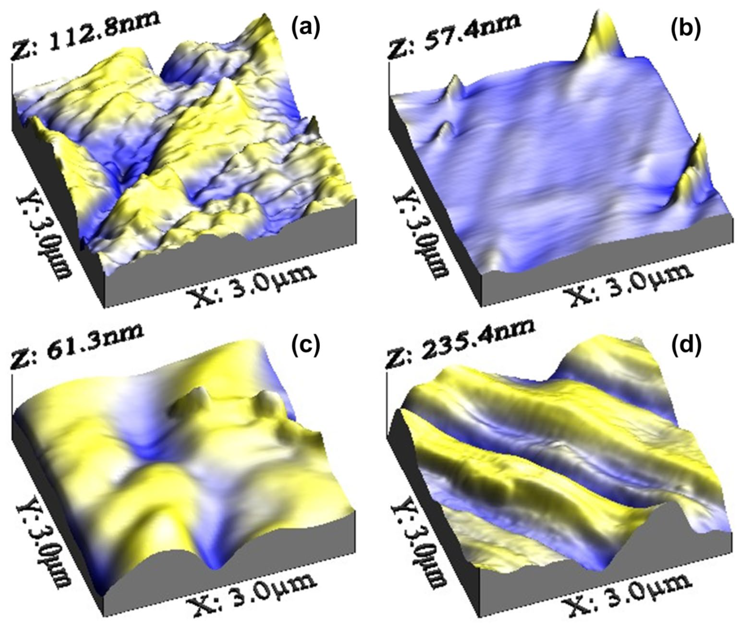
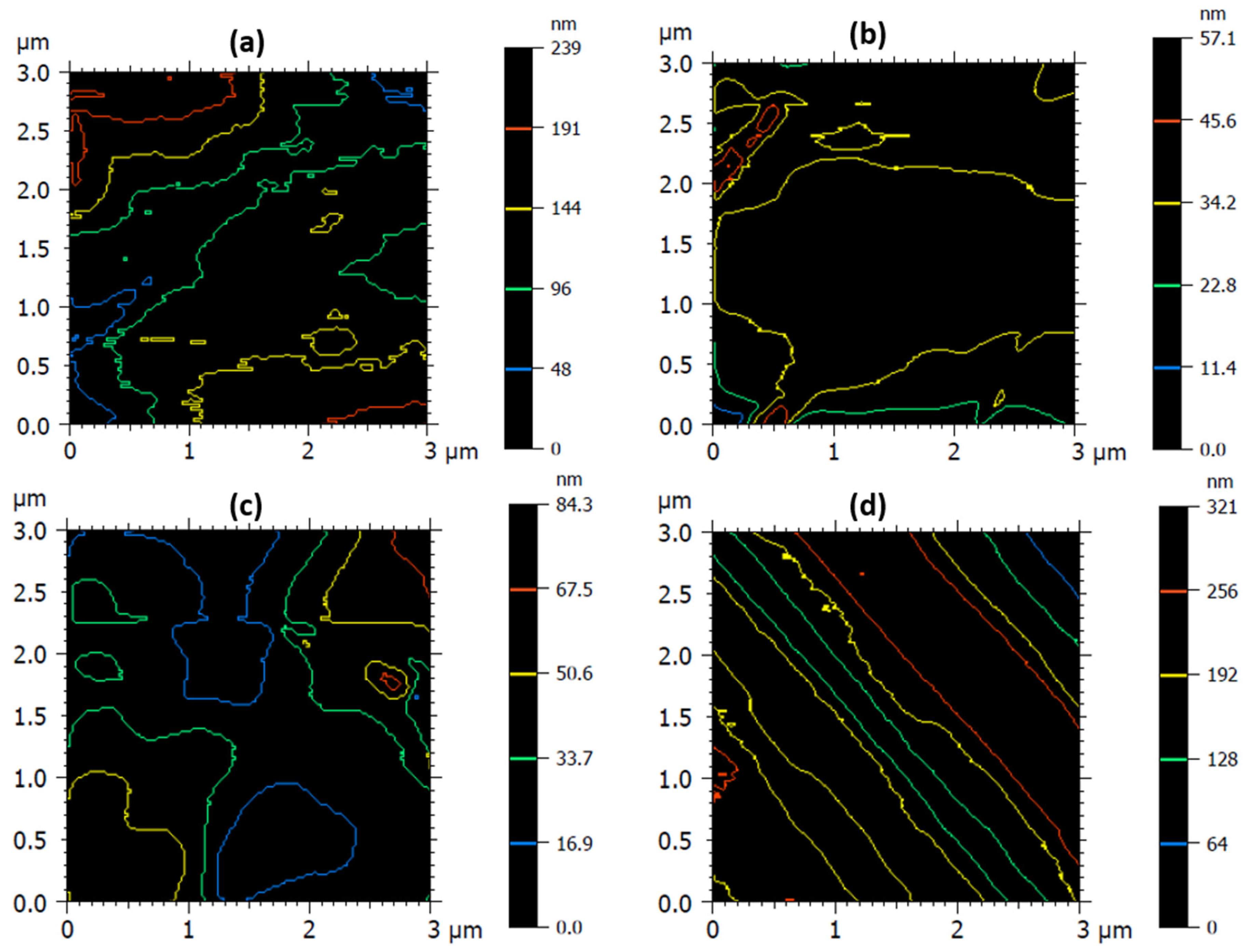
3.1. Standard Morphology Analysis

Three-dimensional topographies via Atomic Force Microscopy (AFM) of the samples S1, S2, S3 and S4 are shown in Figure 1. Square areas of 3 µm × 3 µm of the zirconia disc surfaces subjected to different laser treatments were scanned. Actually, processing conditions influence surface texture and changes can be monitored through statistical parameters calculated from AFM data.

The laser treatments provided different topographical features formed by hills (local maxima) and valleys (local minima) of varying amplitudes and spacing, as shown in the two-dimensional profiles (Rz’s) of Figure 2.

The amplitude parameters (

Table 1. Amplitude parameters of the samples, according to ISO 25178-2:2012.

Parameter	Unit	S1	S2	S3	S4
Sq	[nm]	14.13 ± 2.6	3.247 ± 0.3	7.097 ± 0.5	35.07 ± 2.7
Sp	[µm]	46.50 ± 3.1	32.38 ± 2.7	26.33 ± 2.6	103.5 ± 4.2
Sv	[µm]	66.30 ± 3.9	25.01 ± 2.6	34.92 ± 2.7	131.9 ± 4.4
Sz	[µm]	112.8 ± 4.3	57.39 ± 2.9	61.25 ± 2.9	235.4 ± 6.8

), obtained from the AFM data, showed that treatments with Nd-YAG (S2) and Er-YAG (S3) lasers reduce the surface roughness of the Zirconia ceramics disc, while the CO₂ laser treatment has the opposite effect. The S2 sample presented the lowest values of root mean square roughness (Sq = 3.247 nm), maximum pit height (Sv = 25.01 nm) and maximum height (Sz = 57.39 nm). On the other hand, sample S4 presented values of Sq, Sp, Sv and Sz, equivalent to more than twice the value presented by the reference sample (S1). The CO₂ laser (wavelength 10.16 μm) has a much longer wavelength than the Nd-YAG (wavelength 2.94 μm) and Er-YAG (wavelength 1.064 μm) lasers [29]. The significant difference presented in amplitude parameters by sample S4 in relation to samples S2 and S3 can be associated with this fact.

MountainsMap^® Premium 8.1 software was used to render the topographical maps obtained by AFM (Figure 3 and Figure 4) [30]. The renderings show representative furrows on sample surfaces, revealing that they are dominated by similar channel systems with apparent furrow uniformity, mainly sample S4 (CO₂ laser treatment).

The maximum depth of furrow and mean depth of furrow parameters, presented in

Table 2. Furrow parameters of the samples, according to ISO 25178-2:2012.

Parameter	Unit	S1	S2	S3	S4
Maximum depth of furrows	nm	39.2 ± 2.9	14.8 ± 1.8	14 ± 1.8	85.4 ± 5.7
Mean depth of furrows	nm	15.2 ± 1.8	3.92 ± 0.3	5.71 ± 0.5	20.1 ± 1.9
Mean density of furrows	cm/cm2	36,208 ± 215	45,410 ± 284	27,721 ± 187	43,765 ± 275

, increased from S1 (reference sample) to S4, confirming the behavior indicated by the amplitude parameters (Table 1). Overall, the results in Table 2 suggest that Nd-YAG (S2) and Er-YAG (S3) laser treatments smooth the topography of the Zirconia disc surface, while CO₂ laser treatment has the opposite effect. Furthermore, Figure 4 shows that the S4 treatment was the one that caused the greatest changes in the topography boundary pattern.

3.2. Spatial Autocorrelation (ACF) and Moran’s Correlogram

Autocorrelation analysis is a statistical method used for analysis of repeating patterns in topographic data [33]. One-dimensional autocorrelation is interesting, but in some cases, the two-dimensional autocorrelation is more useful for AFM images. The ACF is shown in real space, so the spacing of the repeating features (correlation length) can then be measured directly from the image. Two-dimensional autocorrelation analysis for the fast decay (black line) and slow decay (red line) direction of the samples is shown in Figure 5.

The correlation length (r) is calculated using a Gaussian fit over the ACF and represents the distance at which the repetition pattern is maintained. Actually, different topographic directions can display different values for this parameter. Thus, to assess the texture isotropy of the surface, the texture–aspect ratio (Str) must be calculated. If Str is close to unity, then the surface is isotropic, that is, it has the same repetition patterns, regardless of the direction. If Str is close to 0, then the surface is anisotropic, that is, it has a texture direction with a dominant repeating pattern [34].

Table 3. The fastest (θ_min) and the slowest (θ_max) decay directions of the autocorrelation function (ACF), correlation length for both directions (r_min and r_max) and texture–aspect ratio (Str) for the investigated samples.

Parameter	Unit	S1	S2	S3	S4
θmin	[°]	−10.01	−41.42	−14.86	31.50
θmax	[°]	47.26	51.93	−89.65	−45.00
rmin	[nm]	303.3	132.8	297.0	213.0
rmax	[nm]	630.3	617.7	966.8	2113
Str	[-]	0.4815 ± 0.091	0.2151 ± 0.052	0.3072 ± 0.074	0.1008 ± 0.021

shows the values of the correlation parameters obtained from the ACF in Figure 3a–d. All laser treatments reduced the superficial isotropy of zirconia ceramic sample S4 (CO₂ laser treatment), which was the one that caused the greatest effect, with an Str value almost 4× lower than the reference sample (S1). The Er-YAG laser treatment (S3) had the least significant effect on the Str value, showing a reduction of approximately 63%. However, samples S3 (r_max = 966.8 nm) and S4 (r_max = 2113 nm) showed much greater maximum correlation lengths than S1 (r_max = 630.3 nm), while sample S2 (r_max = 617.7 nm) showed a small reduction in relation to S1.

To evaluate, in more detail, the spatial autocorrelation of the topography, it is interesting to obtain Moran’s correlograms of the images (Figure 6). Such a correlogram is a graph of the Moran index versus distance lags. The Moran index (I) ranges from −1 to 1. For topography data, I = 0 reveals perfect randomness of height distribution. A I > 0 indicates the grouping degree of similar heights and a perfect clustering when I = 1. On the other hand, I < 0 demonstrates the grouping degree of different heights and represents an ideal dispersion when I = −1. Furthermore, it can be said that the Moran index is a short-range correlation measure, since the Moran correlogram shows that the I index decreases with the distance lag [35,38]. The Moran index was calculated over the entire data matrix extracted from the AFM image, which makes this parameter very interesting for differentiating spatial patterns. In this context, the graph in Figure 6 shows that all surfaces present a high degree of clustering. However, the S4 surface (CO₂ laser treatment) is the one that loses correlation faster for distant neighborhoods. In contrast, treatment with the Er-YAG laser (S3 surface) showed a behavior very close to the reference sample (S1). Such results are in agreement with the ACF in Figure 5 and reaffirm the hypothesis that the treatment with CO₂ laser is the one that causes the greatest change in the surface of the zirconia disc.

3.3. Minkowski Functionals

Minkowski functionals (MFs) are morphological measures usually defined for binary systems. Hence, the AFM images to be analyzed need to be segmented into peaks and valleys through a threshold. The MFs can be used to describe both the morphology (shape) and topology (connectedness) of a system [39,40]. Figure 7 shows graphs of Minkowski Functionals (MFs) as a function of different thresholds (z). In panel (a), we see that the Minkowski volume (V) is a decreasing function with the threshold z for all samples. This is an expected feature since it is a measure of the relative matter amount existing above the threshold z. More interestingly, we observe that all treated samples have an enhancement in the decreasing rate of V versus z. In panel (b,c), we note that all laser treatments induced changes in the Minkowski boundary (S) and Minkowski connectivity (χ), suggesting modifications to the connectedness of the surface.

Table 4. Minkowski functionals (MFs) for the images binarized using the median of the z values as thresholds. Minkowski volume (V), Minkowski boundary (S) and Minkowski connectivity (χ).

Parameter	Unit	S1	S2	S3	S4
V	[-]	0.767	0.043	0.745	0.660
S [10−3]	[-]	0.043	0.011	0.021	0.036
χ [10−6]	[-]	−0.0003	9.16 × 10−5	−6.10 × 10−5	−7.63 × 10−5

shows the values of the Minkowski Functionals (MFs) for the images binarized by the median of the z values. According to Salerno and Banzato [40], the most natural choice for the thresholding value z for MFs is taking it as equal to the median value of the scanned z range. All laser treatments reduced the amount of matter in the peaks, especially for the S2 surface (Nd-YAG laser treatment), which presented a Minkowski volume value almost 18-times smaller than the reference sample (S1). Laser treatments also reduced the Minkowski surface, with an emphasis, again, on sample S2, which showed a reduction of almost 4× the value of sample S1. Thus, on all treated surfaces, there was a decrease in spiky isolated regions. Regarding the Minkowski connectivity, only the S2 surface presented a positive value (χ > 0), indicating a punctiform structure, which is in accordance with Figure 1b. All other samples showed χ < 0, which is characteristic of a porous structure, corroborating Figure 1a–d.

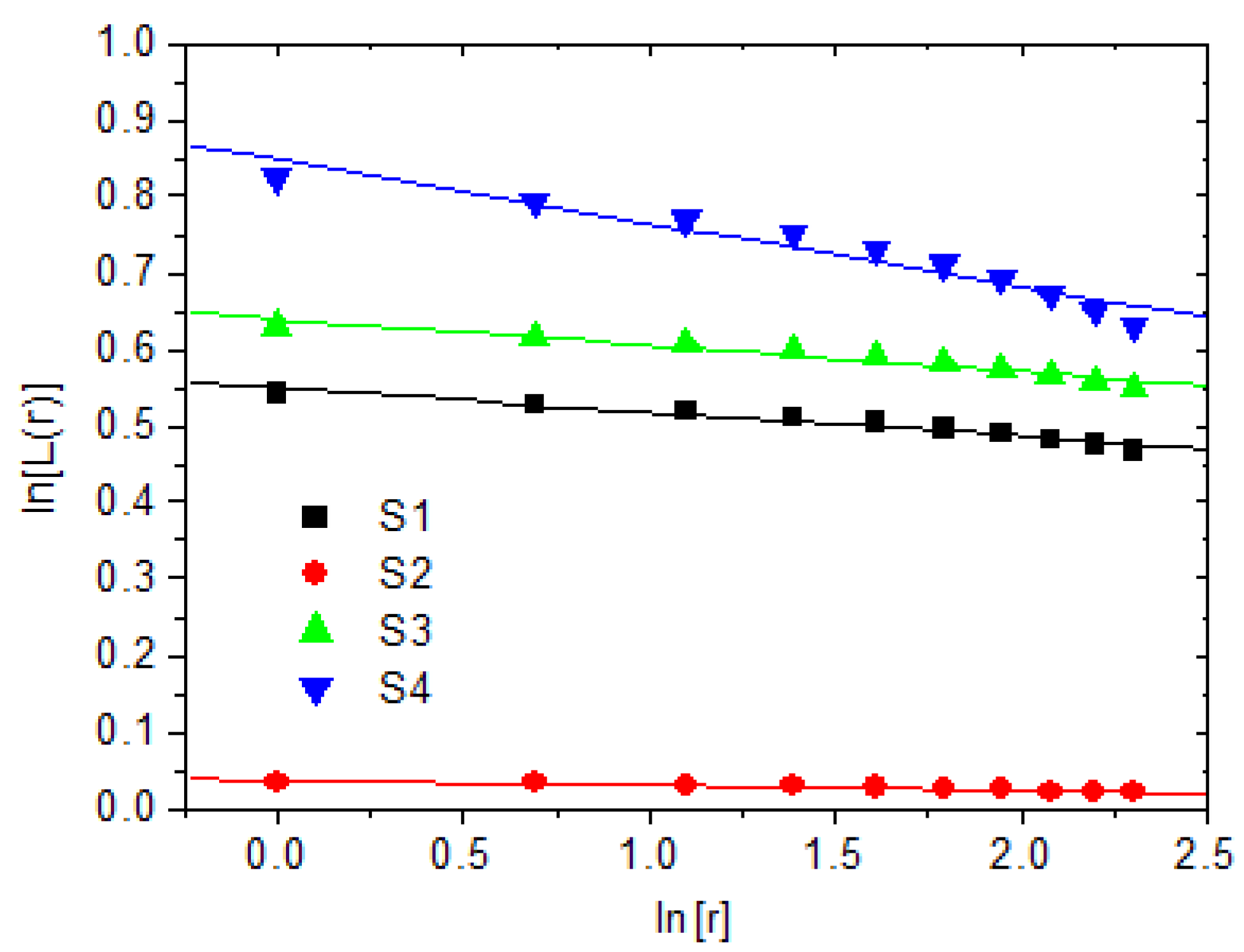
3.4. Fractal Analysis

The spatial autocorrelation of the samples, which was confirmed by the ACF (Figure 5) and by Moran’s correlograms (Figure 6), suggests that the surfaces evaluated have characteristics similar to self-affine fractals. Thus, the analysis fractal of the samples was performed by calculating the parameters: fractal dimension (FD), fractal succolarity (FS) and lacunarity exponent (β). FD is a measure of complexity referring to the distribution of heights on the surface and it is related to the filling of the metric space of the topography. The FS assesses the connection between the upper and lower bands of the scanned region, that is, it is an indirect measure of percolation. β is a useful parameter to assess the homogeneity of lacuna distribution as well as its size on the surface of the samples. Figure 8 shows plots of the lacunarity distribution of the samples, where the lacunarity exponent is equal to the slope of the linear fit for lacunarity value L(r) versus length of box (r).

The calculated fractal parameters are shown in

Table 5. Fractal parameters of the samples.

Parameter	Unit	S1	S2	S3	S4
FD	[-]	2.183	2.067	2.089	2.15
FS	[-]	0.601	0.976	0.533	0.448
β	[-]	0.032	0.007	0.035	0.083

. As can be seen, all laser treatments reduced the surface complexity of the Zirconia ceramic disc. Treatment with the Nd-YAG laser (S2) had the greatest effect, showing a reduction of approximately 5.3% in the FD value. On the other hand, surface percolation (evaluated by the value of FS) increased by almost 33% for sample S2 and decreased by almost 21% for sample S4 (CO₂ laser treatment). All samples showed a high degree of surface microtexture homogeneity (β < 0.09), with emphasis for sample S2, which presented the lowest value of lacunarity exponent (β = 0.007), and sample S4, which showed an increase of approximately 1.6× in relation to the β value of the surface of S1 (reference sample). Er-YAG laser treatment (S3) had an intermediate effect on the fractal aspects of the samples (Table 4). According to the range of values presented on the vertical axis of the graph in Figure 6, the CO₂ laser treatment (S4) provided the largest lacunas sizes, while the Nd-YAG laser treatment (S2) formed a surface with significantly smaller lacunas than S1, S3 and S4 samples. This is supported, considering that a surface topography is more lacunar for larger values of L(r) [32].

3.5. Multifractal Analysis

Multifractal analysis was applied to the AFM images using MATLAB R2015b software. More specifically, the box-counting method was used to investigate the multifractality of the surfaces [41,42,43]. A multifractal structure could be seen as an extension of the fractal structure [44]. Multifractal spectrum identifies the fluctuations in fractal structure, e.g., in multifractal analysis, we want to determine whether some type of power-law scaling exists for various statistical moments at different scales. Thus, if this scaling behavior is characterized by a single scaling exponent, or equivalently is a linear function of the moments, the process is monofractal (or fractal). However, if the scaling behavior by scale is a nonlinear function of the moments, the process is multifractal [41,42,43,44,45], which is our present case, as shown in Figure 9.

Table 6. Measures of multifractal spectra.

Parameter	S1	S2	S3	S4
f(αmax)	2.007	1.316	1.944	2.002
f(αmin)	0.143	−0.207	−0.153	−0.185
Δf = f(αmax) − f(αmin)	1.864	1.523	2.097	2.187
αmax	3.184	3.540	3.513	3.485
αmin	2.137	2.046	2.128	2.131
Δα = αmax − αmin	1.047	1.494	1.385	1.354

shows the multifractal parameters obtained from the multifractal spectra of the samples. The heterogeneity in the topographies can be assessed by the magnitude of differences in the values of f(α_max) and f(α_min) or in the values of α_max and α_min. Actually, Δf on the vertical axis and Δα on the horizontal axis indicate the heterogeneity degree in the samples, which can be further used to differentiate the type and size of singularities in AFM image profiles. The Δα values show that the multifractality of the surface of the Zirconia disc increases for all laser treatments, that is, the samples start to have greater spatial variability in their height values. However, sample S2 (Nd-YAG laser treatment) had its multifractal spectrum strongly affected by the low volume of matter in the peaks and its point structure, as confirmed by the Minkowski functionals (Figure 7 and Table 4). This sample showed ambiguity between the values of Δf and Δα. On the other hand, through the analysis of lacunarity and the measurements of the lacunarity exponent (β) (Figure 8 and Table 5), it was possible to perceive that the parameter Δf is the most suitable to evaluate the multifractality in our samples, since it agrees with the β values. Thus, it can be concluded that the CO₂ laser treatment (S4) has a multifractality that increases by about 32% compared to the reference sample (S1). In contrast, Nd-YAG laser treatment (S2) reduces Zirconia ceramic disc multifractality by almost 34%. The Er-YAG laser treatment (S3) showed an intermediate behavior, corroborating our monofractal analysis.

4. Conclusions

We propose the application of morphological, fractal and multifractal analysis to differentiate surface patterns on zirconia-based ceramics after laser treatments. Furthermore, we introduce two new approaches for ceramic surfaces: the Moran correlogram, which complements the spatial autocorrelation analyses, and the Otsu binarization algorithm, which was used to identify the lacunar points in the lacunarity analysis. Initial insights were gained from AFM images that revealed that all treated surfaces have significant differences in relation to the reference samples. Quantitatively, spatial surface texture parameters revealed that all laser treatments decreased the superficial isotropy of Zirconia disc, where the most noticeable decrease occurred with CO₂ laser treatment. In turn, Moran’s correlograms showed that the short-range correlation decreased for all treated surfaces, where the fattest decrease occurred again with CO₂ laser treatment. The MFs indicated a reduction in the amount of matter in the peaks, especially for the sample with Nd-YAG laser treatment. Moreover, the FD measurements detected a reduction in the topographic complexity of all treated samples, where the sample treated with a CO₂ laser showed the smallest drop in the FD. On the other hand, clear fingerprints of multifractal behavior in all the samples were detected, where the highest degree of multifractality was computed for the sample treated with the CO₂ laser. Finally, our findings suggested that the morphological changes caused by laser treatments on the surfaces of zirconia discs can be monitored and differentiated through the parameters proposed here.

References

1. Han, J.; Zhang, F.; Van Meerbeek, B.; Vleugels, J.; Braem, A.; Castagne, S. Laser Surface Texturing of Zirconia-Based Ceramics for Dental Applications: A Review. Mater. Sci. Eng. C 2021, 123, 112034. [Google Scholar] [CrossRef] [PubMed]
2. Osman, R.; Swain, M. A Critical Review of Dental Implant Materials with an Emphasis on Titanium versus Zirconia. Materials 2015, 8, 932–958. [Google Scholar] [CrossRef] [PubMed]
3. Yoshinari, M. Future Prospects of Zirconia for Oral Implants—A Review. Dent. Mater. J. 2020, 39, 37–45. [Google Scholar] [CrossRef] [PubMed]
4. Elnayef, B.; Lázaro, A.; Suárez-López del Amo, F.; Galindo-Moreno, P.; Wang, H.-L.; Gargallo-Albiol, J.; Hernández-Alfaro, F. Zirconia Implants as an Alternative to Titanium: A Systematic Review and Meta-Analysis. Int. J. Oral Maxillofac. Implants 2017, 32, e125–e134. [Google Scholar] [CrossRef]
5. Faria, D.; Madeira, S.; Buciumeanu, M.; Silva, F.S.; Carvalho, O. Novel Laser Textured Surface Designs for Improved Zirconia Implants Performance. Mater. Sci. Eng. C 2020, 108, 110390. [Google Scholar] [CrossRef]
6. Fattahi, M.; Nezafat, N.B.; Ţălu, Ş.; Solaymani, S.; Ghoranneviss, M.; Elahi, S.M.; Shafiekhani, A.; Rezaee, S. Topographic Characterization of Zirconia-Based Ceramics by Atomic Force Microscopy: A Case Study on Different Laser Irradiations. J. Alloys Compd. 2020, 831, 154763. [Google Scholar] [CrossRef]
7. Sennerby, L.; Dasmah, A.; Larsson, B.; Iverhed, M. Bone Tissue Responses to Surface-Modified Zirconia Implants: A Histomorphometric and Removal Torque Study in the Rabbit. Clin. Implant Dent. Relat. Res. 2005, 7, s13–s20. [Google Scholar] [CrossRef]
8. Gahlert, M.; Gudehus, T.; Eichhorn, S.; Steinhauser, E.; Kniha, H.; Erhardt, W. Biomechanical and Histomorphometric Comparison between Zirconia Implants with Varying Surface Textures and a Titanium Implant in the Maxilla of Miniature Pigs. Clin. Oral Implants Res. 2007, 18, 662–668. [Google Scholar] [CrossRef]
9. Park, Y.-S.; Chung, S.-H.; Shon, W.-J. Peri-Implant Bone Formation and Surface Characteristics of Rough Surface Zirconia Implants Manufactured by Powder Injection Molding Technique in Rabbit Tibiae. Clin. Oral Implants Res. 2013, 24, 586–591. [Google Scholar] [CrossRef]
10. Delgado-Ruíz, R.; Markovic, A.; Calvo-Guirado, L.; Lazic, Z.; Piattelli, A.; Boticelli, D.; Maté-Sánchez, J.; Negri, B.; Ramírez-Fernández, M.; Misic, T. Implant Stability and Marginal Bone Level of Microgrooved Zirconia Dental Implants: A 3-Month Experimental Study on Dogs. Vojnosanit. Pregl. 2014, 71, 451–461. [Google Scholar] [CrossRef] [Green Version]
11. Tzanakakis, E.-G.C.; Tzoutzas, I.G.; Koidis, P.T. Is There a Potential for Durable Adhesion to Zirconia Restorations? A Systematic Review. J. Prosthet. Dent. 2016, 115, 9–19. [Google Scholar] [CrossRef]
12. Kim, H.-K.; Woo, K.M.; Shon, W.-J.; Ahn, J.-S.; Cha, S.; Park, Y.-S. Comparison of Peri-Implant Bone Formation around Injection-Molded and Machined Surface Zirconia Implants in Rabbit Tibiae. Dent. Mater. J. 2015, 34, 508–515. [Google Scholar] [CrossRef]
13. Hempel, U.; Hefti, T.; Kalbacova, M.; Wolf-Brandstetter, C.; Dieter, P.; Schlottig, F. Response of Osteoblast-like SAOS-2 Cells to Zirconia Ceramics with Different Surface Topographies. Clin. Oral Implants Res. 2010, 21, 174–181. [Google Scholar] [CrossRef]
14. Calvo-Guirado, J.L.; Aguilar Salvatierra, A.; Gargallo-Albiol, J.; Delgado-Ruiz, R.A.; Maté Sanchez, J.E.; Satorres-Nieto, M. Zirconia with Laser-Modified Microgrooved Surface vs. Titanium Implants Covered with Melatonin Stimulates Bone Formation. Experimental Study in Tibia Rabbits. Clin. Oral Implants Res. 2015, 26, 1421–1429. [Google Scholar] [CrossRef]
15. Wang, G.; Meng, F.; Ding, C.; Chu, P.K.; Liu, X. Microstructure, Bioactivity and Osteoblast Behavior of Monoclinic Zirconia Coating with Nanostructured Surface. Acta Biomater. 2010, 6, 990–1000. [Google Scholar] [CrossRef]
16. Hao, L.; Ma, D.R.; Lawrence, J.; Zhu, X. Enhancing Osteoblast Functions on a Magnesia Partially Stabilised Zirconia Bioceramic by Means of Laser Irradiation. Mater. Sci. Eng. C 2005, 25, 496–502. [Google Scholar] [CrossRef]
17. Cheng, J.; Liu, C.; Shang, S.; Liu, D.; Perrie, W.; Dearden, G.; Watkins, K. A Review of Ultrafast Laser Materials Micromachining. Opt. Laser Technol. 2013, 46, 88–102. [Google Scholar] [CrossRef]
18. Mirhashemi, A.; Emadian Razavi, E.s.; Behboodi, S.; Chiniforush, N. Effect of Laser-Assisted Bleaching with Nd:YAG and Diode Lasers on Shear Bond Strength of Orthodontic Brackets. Lasers Med. Sci. 2015, 30, 2245–2249. [Google Scholar] [CrossRef]
19. Mohammad Asnaashari, M.M. Effectiveness of Lasers in the Treatment of Dentin Hypersensitivity. J. Lasers Med. Sci. 2013, 4, 1–7. [Google Scholar]
20. Marcondes, M.; Gandolfi Paranhos, M.P.; Spohr, A.M.; Mota, E.G.; Lima da Silva, I.N.; Souto, A.A.; Burnett, L.H. The Influence of the Nd:YAG Laser Bleaching on Physical and Mechanical Properties of the Dental Enamel. J. Biomed. Mater. Res. Part B Appl. Biomater. 2008, 90, 388–395. [Google Scholar] [CrossRef]
21. Michiels, R.; Vergauwen, T.E.M.; Mavridou, A.; Meire, M.; De Bruyne, M.; De Moor, R.J.G. Investigation of Coronal Leakage of Root Fillings after Smear-Layer Removal with EDTA or Nd:YAG Lasing through Capillary-Flow Porometry. Photomed. Laser Surg. 2010, 28, S-43–S-50. [Google Scholar] [CrossRef] [PubMed] [Green Version]
22. Singhvi, R.; Stephanopoulos, G.; Wang, D.I.C. Effects of Substratum Morphology on Cell Physiology. Biotechnol. Bioeng. 1994, 43, 764–771. [Google Scholar] [CrossRef] [PubMed]
23. Curtis, A.; Wilkinson, C. Topographical Control of Cells. Biomaterials 1997, 18, 1573–1583. [Google Scholar] [CrossRef] [PubMed]
24. Zhou, W.; Cao, Y.; Zhao, H.; Li, Z.; Feng, P.; Feng, F. Fractal Analysis on Surface Topography of Thin Films: A Review. Fractal Fract. 2022, 6, 135. [Google Scholar] [CrossRef]
25. Mwema, F.M.; Jen, T.-C.; Kaspar, P. Fractal Theory in Thin Films: Literature Review and Bibliometric Evidence on Applications and Trends. Fractal Fract. 2022, 6, 489. [Google Scholar] [CrossRef]
26. Gavriil, V.; Chatzichristidi, M.; Kollia, Z.; Cefalas, A.-C.; Spyropoulos-Antonakakis, N.; Semashko, V.; Sarantopoulou, E. Photons Probe Entropic Potential Variation during Molecular Confinement in Nanocavities. Entropy 2018, 20, 545. [Google Scholar] [CrossRef]
27. Spyropoulos-Antonakakis, N.; Sarantopoulou, E.; Trohopoulos, P.N.; Stefi, A.L.; Kollia, Z.; Gavriil, V.E.; Bourkoula, A.; Petrou, P.S.; Kakabakos, S.; Semashko, V.V.; et al. Selective Aggregation of PAMAM Dendrimer Nanocarriers and PAMAM/ZnPc Nanodrugs on Human Atheromatous Carotid Tissues: A Photodynamic Therapy for Atherosclerosis. Nanoscale Res. Lett. 2015, 10, 210. [Google Scholar] [CrossRef]
28. Starodubtseva, M.N.; Starodubtsev, I.E.; Starodubtsev, E.G. Novel Fractal Characteristic of Atomic Force Microscopy Images. Micron 2017, 96, 96–102. [Google Scholar] [CrossRef]
29. Yamada, M.K.; Uo, M.; Ohkawa, S.; Akasaka, T.; Watari, F. Three-Dimensional Topographic Scanning Electron Microscope and Raman Spectroscopic Analyses of the Irradiation Effect on Teeth by Nd:YAG, Er: YAG, and CO2 Lasers. J. Biomed. Mater. Res. 2004, 71, 7–15. [Google Scholar] [CrossRef]
30. Ghaderi, A.; Shafiekhani, A.; Solaymani, S.; Ţălu, Ş.; da Fonseca Filho, H.D.; Ferreira, N.S.; Matos, R.S.; Zahrabi, H.; Dejam, L. Advanced Microstructure, Morphology and CO Gas Sensor Properties of Cu/Ni Bilayers at Nanoscale. Sci. Rep. 2022, 12, 12002. [Google Scholar] [CrossRef]
31. Dong, W.P.; Sullivan, P.J.; Stout, K.J. Comprehensive Study of Parameters for Characterising Three-Dimensional Surface Topography. Wear 1994, 178, 45–60. [Google Scholar] [CrossRef]
32. Pinto, E.P.; Pires, M.A.; Matos, R.S.; Zamora, R.R.M.; Menezes, R.P.; Araújo, R.S.; de Souza, T.M. Lacunarity Exponent and Moran Index: A Complementary Methodology to Analyze AFM Images and Its Application to Chitosan Films. Phys. A Stat. Mech. Appl. 2021, 581, 126192. [Google Scholar] [CrossRef]
33. Nečas, D.; Klapetek, P. One-Dimensional Autocorrelation and Power Spectrum Density Functions of Irregular Regions. Ultramicroscopy 2013, 124, 13–19. [Google Scholar] [CrossRef]
34. Matos, R.S.; Pinto, E.P.; Ramos, G.Q.; Fonseca de Albuquerque, M.D.; Fonseca Filho, H.D. Stereometric Characterization of Kefir Microbial Films Associated with Maytenus Rigida Extract. Microsc. Res. Tech. 2020, 83, 1401–1410. [Google Scholar] [CrossRef]
35. Cocu, N.; Harrington, R.; Hullé, M.; Rounsevell, M.D.A. Spatial Autocorrelation as a Tool for Identifying the Geographical Patterns of Aphid Annual Abundance. Agric. For. Entomol. 2005, 7, 31–43. [Google Scholar] [CrossRef]
36. Ţălu, Ş.; Stach, S.; Mahajan, A.; Pathak, D.; Wagner, T.; Kumar, A.; Bedi, R.K. Multifractal Analysis of Drop-Casted Copper (II) Tetrasulfophthalocyanine Film Surfaces on the Indium Tin Oxide Substrates. Surf. Interface Anal. 2014, 46, 393–398. [Google Scholar] [CrossRef]
37. Zelati, A.; Mardani, M.; Rezaee, S.; Matos, R.S.; Pires, M.A.; da Fonseca Filho, H.D.; Das, A.; Hafezi, F.; Rad, G.A.; Kumar, S.; et al. Morphological and Multifractal Properties of Cr Thin Films Deposited onto Different Substrates. Microsc. Res. Tech. 2022, 86, 157–168. [Google Scholar] [CrossRef]
38. Chen, Y. New Approaches for Calculating Moran’s Index of Spatial Autocorrelation. PLoS ONE 2013, 8, e68336. [Google Scholar] [CrossRef]
39. Boelens, A.M.P.; Tchelepi, H.A. QuantImPy: Minkowski Functionals and Functions with Python. SoftwareX 2021, 16, 100823. [Google Scholar] [CrossRef]
40. Vogel, H.-J.; Weller, U.; Schlüter, S. Quantification of Soil Structure Based on Minkowski Functions. Comput. Geosci. 2010, 36, 1236–1245. [Google Scholar] [CrossRef]
41. Ţălu, Ş.; Boudour, S.; Bouchama, I.; Astinchap, B.; Ghanbaripour, H.; Akhtar, M.S.; Zahra, S. Multifractal Analysis of Mg-doped ZnO Thin Films Deposited by Sol–Gel Spin Coating Method. Microsc. Res. Tech. 2022, 85, 1213–1223. [Google Scholar] [CrossRef] [PubMed]
42. Salat, H.; Murcio, R.; Arcaute, E. Multifractal Methodology. Phys. A Stat. Mech. Appl. 2017, 473, 467–487. [Google Scholar] [CrossRef]
43. Ihlen, E.A.F. Introduction to Multifractal Detrended Fluctuation Analysis in Matlab. Front. Physiol. 2012, 3, 141. [Google Scholar] [CrossRef] [PubMed]
44. Ţălu, Ş. Micro and Nanoscale Characterization of Three Dimensional Surfaces. Basics and Applications; Napoca Star Publishing House: Cluj-Napoca, Romania, 2015; ISBN 978-606-690-349-3. [Google Scholar]
45. Shakoury, R.; Rezaee, S.; Mwema, F.; Luna, C.; Ghosh, K.; Jurečka, S.; Ţălu, Ş.; Arman, A.; Grayeli Korpi, A. Multifractal and optical bandgap characterization of Ta2O5 thin films deposited by electron gun method. Opt. Quant. Electron. 2020, 52, 95. [Google Scholar] [CrossRef]
Figure 1. 3D AFM images related to the surfaces of zirconia discs with and without laser treatments: (a) S1, (b) S2, (c) S3 and (d) S4.
Fractalfract 07 00160 g001
Figure 2. Rz profile of (a) S1, (b) S2, (c) S3 and (d) S4, respectively.
Fractalfract 07 00160 g002
Figure 3. The representation of the furrows for the samples: (a) S1, (b) S2, (c) S3 and (d) S4.
Fractalfract 07 00160 g003
Figure 4. The graphical representation of the contour lines for the samples: (a) S1, (b) S2, (c) S3 and (d) S4.
Fractalfract 07 00160 g004
Figure 5. The autocorrelation function (ACF) as a function of the correlation length (r) of (a) S1, (b) S2, (c) S3 and (d) S4, respectively.
Fractalfract 07 00160 g005
Figure 6. Moran’s Correlograms: S1, S2, S3 and S4.
Fractalfract 07 00160 g006
Figure 7. The Minkowski functionals (MFs) for different thresholds: (a) Minkowski volume, (b) Minkowski boundary and (c) Minkowski connectivity for the scanning area of 3 μm × 3 μm.
Fractalfract 07 00160 g007
Figure 8. Lacunarity analysis: S1, S2, S3 and S4. All linear fits presented R² > 0.9. R² is the coefficient of determination of the linear fit, the closer to 1 the value of R² is, the better the linear model will be.
Fractalfract 07 00160 g008
Figure 9. (a) Mass exponent τ(q) and (b) generalized dimensions Dq as a function of the order of moments (q) and (c) multifractal spectra (f(α) versus α). For clarity, we shifted the curves S1, S2, S3 and S4, shown in the mass exponent graph, by −5, −1, +3 and +7, respectively.
Fractalfract 07 00160 g009