Article

Numerical Investigation of Fractional Step-Down ELS Option

1
Department of Mathematics and Applied Mathematics, Reading Academy, Nanjing University of Information Science and Technology, Nanjing 210044, China
2
School of Mathematics, Harbin Institute of Technology, Harbin 150001, China
3
School of Economics, Nanjing University of Finance and Economics, Nanjing 210023, China
4
Center for Applied Mathematics of Jiangsu Province, Nanjing University of Information Science and Technology, Nanjing 210044, China
5
Jiangsu International Joint Laboratory on System Modeling and Data Analysis, Nanjing University of Information Science and Technology, Nanjing 210044, China
*
Author to whom correspondence should be addressed.
Current address: School of Mathematics and Statistics, Nanjing University of Information Science and Technology, Nanjing 210044, China.
Fractal Fract. 2023, 7(2), 126; https://doi.org/10.3390/fractalfract7020126
Submission received: 16 December 2022 / Revised: 17 January 2023 / Accepted: 18 January 2023 / Published: 30 January 2023

Abstract

:
In this paper, we use the finite difference methods to explore step-down Equity Linked Securities (ELS) options under the fractional Black-Scholes model. We establish Crank-Nicolson scheme under one asset and study the impact of Hurst exponent (H) on return of repayment under fixed stock price. We also explore the impact of stock price on return of repayment under different H. Through numerical experiments, it is found that the return of repayment of options is related to H, and the result of difference scheme will increase with the increase of H. In the case of two assets, we establish implicit scheme, and in the case of three assets, we use operator splitting method (OSM) method to establish semi-implicit scheme. We get the result that the H also influences the return of repayment in two and three assets. We also conduct Greeks analysis. Through Greeks analysis, we find that the long-term correlation of stocks has a huge impact on investment gains or losses. Therefore, we take historical volatility (fractal exponents) into account which can significantly reduce risk and increase revenue for investors.

1. Introduction

Options originated in the United States and European markets in the late 18th century, but it was not until the 1970s that options trading developed rapidly with the unification and standardization of the trading of options contracts. In recent decades, with the repaid development of economy, the investment risk of financial market is also increasing, and investors are gradually keen to invest in options with hedging, management and analysis function. Therefore, more and more new options have emerged, which not only enrich the financial market, but also meet the needs of a large number of investors to avoid risks. Equity Linked Securities (ELS) is a kind of hybrid debt securities. As one of the most popular derivatives in structured financial instrument, its annual issuance scale exceeds 5 trillion US dollars. Step-down ELS option contains knocks-in and knock-out and the option price will gradually decrease with time. In addition, ELS option products can be based on an underlying asset, such as the Shanghai 50 index. It can also be based on two or three basic assets at the same time, such as Shanghai 50 index, Kospi 200 index, Hang Seng index, etc. Chen and Kensinger [1] studied the pricing of American ELS options and found that the variable interest paid by ELS is related to the performance of S & P 500 stock market index. Baubonis et al. [2] used numerical algorithm to price ELS options. After that, Kim et al. [3] used a new finite difference method to solve the three assets pricing problem based on the operator splitting method which is used by Jeong et al. [4].
Bachelier [5] established many bond price motion models under Brown motion to describe the price return of stock. Because of the negative value of the results obtained from the Brownian motion, Sumuelson [6] proposed a geometric Brownian motion model. Since the 1970s, Black and Scholes [7] gave European call option pricing formula, the research results of options have been increasing, but the results of option pricing research are mainly obtained under the geometric Brownian motion. But in reality, the changes of the target asset price described by the traditional geometric Brownian motion are not necessarily satisfied with the normal, independent increment and continuous path. Mandelbrot and Ness [8] proved that the distribution of capital market income is not symmetrical and does not obey normal distribution. Therefore, some scholars have focused on the study of options under fractional Brownian motion [9,10] or improve reaserch methods [11]. Peter [12] considered that the characteristics of fractional Brownian motion, such as long memory, thick tail and self similarity, can describe the changes of asset prices in financial markets, and puts forward the fractal market hypothesis. Seidler [13] had proved in his paper that the logarithmic return of financial assets has the characteristics of asymmetry, peak and thick tail, capital market mutation or reversal, deviation and so on. But compared with the traditional Brownian motion, the fractional Brownian motion can well describe these characteristics. At the same time, many financial products in financial market have fractal structure [14,15,16,17]. Necula [18] studied European option under fractional Brownian motion and gave the corresponding pricing formula. Liu and Yang [19] studied the European option on dividend-paying stock under fractional Brownian motion which is a new option form. Murwaningtyas et al. [20] studied the European option pricing problem under mixed fractional Brownian motion which includes fractional and geometric, and took the method based on Fourier transformation and quasi conditional expectation to solve the problem. Finally, them gave a formula to calculate the European call option. Jian Wang et al. [21] used Monte Carlo method to study ELS options under fractional Brownian motion and compared the results with those of ELS options and actual results under traditional geometric Brownian motion. Ali et al. [22] developed new group iterative schemes for the numerical solution of two-dimensional anomalous fractional sub-diffusion equation subject to specific initial and Dirichlet boundary conditions. Oderinu et al. [23] considered the nature of these time-fractional differential equations are in sense of Caputo. Nikan et al. [24] addressed the solution of the Rayleigh–Stokes problem for an edge in a generalized Oldroyd-B fluid using fractional derivatives and the radial basis function-generated finite difference (RBF-FD) method. Golbabai et al. [25] considered a partial integro-differential equation (PIDE) problem with a free boundary. Golbabai et al. [26] provided methods for accurate modeling of anomalous diffusion and transport dynamics in determined multifaceted systems. Golbabai et al. [27] investigated the pricing of double barrier options when the price change of the underlying is considered as a fractal transmission system. Golbabai et al. [28] managed to determine the numerical solution of the time fractional Black–Scholes model (TFBSM) by using a truly mesh-free scheme. Nikan et al. [29] proposed an efficient and modified local mesh-less method for the numerical simulation of the TFBSE.
The results of fractional Brownian motion are more close to the actual results. It also shows that the asymmetry, peak thick tail and bias of fractional Brownian motion are more in line with the actual situation. Therefore, we consider the finite difference method to study ELS option under fractional Brownian motion. In order to better observe the financial market, issues must be considered in actual operations. At present, under the environment of the rapid economic development, various financial markets gradually become active, and the demand for investment continues to increase. The resource allocation has become very important. According to the efficiency and risk characteristics of the markets, investors can better price assets, optimize the risk control and perfect their investment portfolios more reasonably with the model we proposed. The efficiency of the market can be used in the pricing of assets and the allocation of resources. Its importance is self-evident in the financial market. Notice that the financial market is not simple linear, it has a complex structure inside, and the fractal market hypothesis can describe the nonlinear structure inside the market. Therefore our model can identify the market much more accurately and can benefit investors profoundly.
The structure and content of this paper are as follows. In Section 2, we give the definition of fractional Brownian motion and establish the mathematical model of fractional step-down ELS. In Section 3, we establish a finite difference scheme for the mathematical model, and carry out numerical experiments in Section 4. Finally, we give the experimental conclusion in Section 5.

2. Fractional Step-Down ELS Model

ELS is a structured product which includes two processes of knock-in and knock-out. Its trading principle is based on financial assets. The return of ELS depends on three forms: early redemption, final redemption and maturity redemption. For one asset, if the price date of the asset at the first exercise is higher than the predetermined exercise price, ELS will give the specified exercise price for early redemption, and the contract will be terminated. Otherwise, the contract will continue to be judged until the next expiration date. If the contract fails to be redeemed in advance when it matures, the return on investment depends on whether the contract meets the knock-in-barrier. When the underlying asset does not reach the knock-in-barrier, ELS gives a fixed value return determined by the fictitious interest rate as the maturity redemption. Otherwise, the final redemption will be made at the asset price on the maturity date.
The trading mechanism of fractional step-down ELS is the same as ELS, only in the holding stage, it meets the conditions of fractional Black-Scholes model. Step-down ELS option means option price gradually decreases with time. Next, we introduce fractional Brownian motion and establish fractional step-down ELS model under different assets, and give the corresponding parameters.

2.1. Fractional Brownian Motion

We suppose that the random process B t , t 0 is Brownian motion, then fractional Brownian motion is to modify B t in Brownian motion to B H t with parameter Hurst exponent (H). H is the earliest statistical measure proposed by Hu and Oksendal [30] applied to fractal analysis. In time series analysis, using H as a measure, we can see how a time series has a long memory and moves irregularly. In fractional Brownian motion, a larger H value indicates a stronger fluctuation trend. Now we define the following: let Ω , F , P be a probability space and H be a constant on 0 , 1 . If the one dimensional Gaussian process satisfies:
  • B 0 H = E B t H , for any t > 0 .
  • E B t H B s H = 1 2 t 2 H + s 2 H t s 2 H , for any t , s > 0 .
The Gaussian process B t H is called fractional Brownian motion with H. E is the mathematical expectation of probability measure p. The function of B t H is:
p B t H B 0 H x = 1 2 π t 2 H S e x p S 2 2 t 2 H d S , t 0 .
At the same time, there are two important properties of fractional Brownian motion.
  • Fractional Brownian motion has self-similarity. For any H 0 , 1 and α > 0 , B α t H and α B t H have the same finite-dimensional distribution.
  • When H = 0.5 , it is the standard Brownian motion. When H > 0.5, B t H has a long-term dependence. When 0 < H < 0.5 , B t H has anti persistence.
If the underlying asset price S t satisfies:
d S t = μ t S t + σ t S t d B t H .
Then S t is said to obey geometric fractional Brownian motion. μ t and σ t represent the forecast return and volatility of the risk asset price respectively. Under the risk neutral measure, μ replaces with risk-free rate r. Equation (2) can be changed to Equation (3):
d S t = r t S t + σ t S t d B t H .
If r t = r and σ t = σ are constants, then Equation (3) can be changed to Equation (4):
d S t = r S t + σ S t d B t H .
We call the underlying asset price S t is an I t o ^ type fractional Black-Scholes market when it satisfies the usual Black-Scholes model conditions and obeys geometric fractional Brownian motion. Hu and Oksendal [30] proved that the market is complete and there is no arbitrage.

2.2. Fractional Step-Down ELS Model of One Asset

We first give the main parameters of fractional step-down ELS option under one asset through Table 1.
In the holding stage, the asset satisfies the fractional Black-Scholes model, therefore, the change of asset satisfies the fractional Black-Scholes partial differential equation (PDE). Through establishing hedge techniques and I t o ^ fractional formula, we can get the fractional Black-Schoels PDE.
V t + H Δ t 2 H 1 S 2 σ 2 2 V S 2 + r S V S r V = 0 .
In Equation (5), V = V S , t represents the return of repayment and Δ t represents time step of T. ϕ S represents V when t = T . To transform the backward-in-time in PDE into forward-in-time, we take τ = T t and obtain the PDE with initial value problem.
V τ = H Δ t 2 H 1 S 2 σ 2 2 V S 2 + r S V S r V , τ 0 , T , S 0 , + , V S , 0 = ϕ S .
In the exercise stage, its judging form is the same as that of ELS. We assume that there are n strike prices, n coupon rates and n strike dates. At the same time, we set S t to represent the value of the underlying asset at time t, S 0 is the price at the initial time, and the above corresponding symbols are:
K 1 K 2 K n , β 1 β 2 β n , δ 1 δ 2 δ n .
It is worth noting that when comparing with the execution price, we use the ratio of the underlying asset price to the initial price. Therefore, judgment conditions of exercise stage can be expressed as follows.
V S , t = F 1 + β 1 , i f S t 1 K 1 , F 1 + β 2 , i f K 2 S t 2 K 1 , D S t 1 K 1 , F 1 + β n , i f K n S t n K 1 , D S t n 1 K n 1 , F 1 + d , o t h e r w i s e .

2.3. Fractional Step-Down ELS Model of Two Assets

In two assets, we let x and y denote the price of two underlying assets and H in x direction and y direction are expressed as H x and H y . The symbols of other parameters remain unchanged. In the holding stage, for x , y Φ , t 0 , T , the return of repayment V x , y , t follows fraction Black-Scholes partial differential equation (PDE):
V t + r x V x + r y V y + H x Δ t 2 H x 1 σ x 2 x 2 V x x
+ H y Δ t 2 H y 1 σ y 2 y 2 V y y + H x + H y Δ t H x + H y 1 ρ x y σ x σ y V x y r V = 0 .
In this equation, σ x , σ y represent the volatility of x and y respectively and ρ x y represents the correlation value between x and y. We also take τ = T t and ϑ x , y represents V when t = T . We obtain the PDE with initial value problem.
V τ = r x V x + r y V y + H x Δ t 2 H x 1 σ x 2 x 2 V x x + H y Δ t 2 H y 1 σ y 2 y 2 V y y + H x + H y Δ t H x + H y 1 ρ x y σ x σ y x y V x y r V , x , y , τ Φ times 0 , T , V x , y , 0 = ϑ x , y .
In the exercise stage, the fractional step-down ELS of two assets is different from that of one asset. The base price of two assets’ fractional step-down ELS is expressed by the minimum value of two underlying assets. If the minimum value is larger than or equal to the strike price at the strike date, the contract will be terminated. If the early redemption fails on the maturity date, the return depends on whether the minimum value of the two underlying assets reaches the knock-in-barrier. Therefore, We take u i = m i n x t i , y t i , i = 1 , 2 , , n and judgment conditions of exercise stage can be expressed as follows.
V x , y , t = F 1 + β 1 , i f u 1 K 1 , F 1 + β 2 , i f K 2 u 2 K 1 , D u 1 K 1 , F 1 + β n , i f K n u n K n 1 K 1 , , D u n 1 K n 1 , F 1 + d , o t h e r w i s e .

2.4. Fractional Step-Down ELS Model of Three Assets

In three assets, we let x, y and z denote the price of three underlying assets and H in direction of x, y and z are expressed as H x , H y and H z . The symbols of other parameters remain unchanged. In the holding stage, for x , y , z Ψ , t 0 , T , the return of repayment V x , y , z , t follows fractional Black-Scholes PDE:
V t + r x V x + r y V y + r z V z
+ H x Δ t 2 H x 1 σ x 2 x 2 V x x + H y Δ t 2 H y 1 σ y 2 y 2 V y y
+ H z Δ t 2 H z 1 σ z 2 z 2 V z z + H x + H y Δ t H x + H y 1 ρ x y σ x σ y x y V x y
+ H y + H z Δ t H y + H z 1 ρ y z σ y σ z y z V y z
+ H x + H z Δ t H x + H z 1 ρ x z σ x σ z x z V x z r V = 0 .
In this equation, σ x , σ y , σ z represent the volatility of x, y and z respectively. ρ x y , ρ y z , ρ z x represent the correlation value between two subscript assets variables. We also take τ = T t and ψ x , y , z represents V when t = T . We obtain the PDE with initial value problem.
V τ = r x V x + r y V y + r z V z + H x Δ t 2 H x 1 σ x 2 x 2 V x x + H y Δ t 2 H y 1 σ y 2 y 2 V y y + H z Δ t 2 H z 1 σ z 2 z 2 V z z + H x + H y Δ t H x + H y 1 ρ x y σ x σ y x y V x y + H y + H z Δ t H y + H z 1 ρ y z σ y σ z y z V y z + H x + H z Δ t H x + H z 1 ρ x z σ x σ z x z V x z r V = 0 , x , y , z , τ Ψ times 0 , T , V x , y , z , 0 = ψ x , y , z .
In the exercise stage, the fractional step-down ELS of three assets is similar to that of two assets. The base price of two assets’ fractional step-down ELS is expressed by the minimum value of three underlying assets. Therefore, judgment conditions of exercise stage can be expressed as follows.
V x , y , z , t = F 1 + β 1 , i f l 1 K 1 , F 1 + β 2 , i f K 2 l 2 K 1 , D l 1 K 1 , F 1 + β n , i f K n l 1 K n 1 K 1 , , D l 1 K n 1 , F 1 + d , o t h e r w i s e ,
where, l i = m i n x t i , y t i , z t i , i = 1 , 2 , , n .

3. Numerical Method

In the holding stage of fractional step-down ELS option. The chang of its return satisfies the fractional Black-Scholes equation. We consider using the finite difference method to solve the initial problem. We establish Crank-Nicolson scheme under one asset and establish implicit scheme under two assets, and in the case of three assets, we use operator splitting method (OSM) method to establish semi-implicit scheme. We also take the judgment condition of the exercise stage and Dirichlet zero boundary as its boundary conditions. On the one asset and two assets, Crank-Nicolson scheme and implicit scheme are unconditionally stable and convergent [31]. On the three asset, OSM method is also proved to be convergent and stable by reference [3,4,32].

3.1. One Underlying Asset

We grid on area Σ : 0 S S m a x , 0 t T . From t = 0 to t = T , we divide the option price into several equal intervals. We take Δ t = T N t , Δ S = S m a x S m i n N S , Δ t represents the time step of T, Δ S represents the price step of S.
There are N t + 1 time periods and N s + 1 option price: 0 , Δ t , 2 Δ t T and 0 , Δ S , , S m a x . In this grid, V i , j denotes the corresponding time i Δ t and option price: j Δ S = S j , where i = 0 , , N t , j = 0 , , N S . We take V j i = V i , j to express the return at point S j . For Equation (6), we consider the Crank-Nicolson scheme.
V j i + 1 V j i Δ t = 1 2 ( H Δ t 2 H 1 σ 2 S j 2 V j + 1 i 2 V j i + V j 1 i Δ S 2
+ r S j V j + 1 i V j 1 i 2 Δ S r V j i ) + 1 2 ( H Δ t 2 H 1 σ 2 S j 2 V j + 1 i + 1 2 V j i + 1 + V j 1 i + 1 Δ S 2
+ r S j V j + 1 i + 1 V j 1 i + 1 2 Δ S r V j i + 1 ) .
After sorting out the above difference scheme and adding zero Dirichilet boundary condition at S = 0 and nonlinear boundary condition at t = T , we can observe the equation as follows:
α j V j 1 i + 1 + B j V j i + 1 + γ j V j + 1 i + 1 = V j i Δ t + H Δ t 2 H 1 σ 2 S j 2 V j + 1 i + 1 2 V j i + 1 + V j 1 i + 1 2 Δ S 2 + r S j V j + 1 i + 1 V j 1 i + 1 4 Δ S r 2 V j i + 1 , 1 j N S 1 , 0 i N t 1 , V j T = ϕ S j , 0 j N S , V S m a x i = V 0 i = V j 0 = 0 , 0 i N t , 0 j N s .
and
α j = r S j 4 Δ S H Δ t 2 H 1 σ 2 S j 2 2 Δ S 2 ,
B j = 1 t + H Δ t 2 H 1 σ 2 S j 2 Δ S 2 + r 2 ,
γ j = r S j 4 Δ S H Δ t 2 H 1 σ 2 S j 2 2 Δ S 2 .
In the system of Equation (9), like ELS option, fractional ELS option has different returns whether the underlying asset occurs knock-in-barrier event. And the boundary conditions at V j T = ϕ S j are also different.
When knock-in-barrier event occurs, ϕ S j can be expressed as:
ϕ S j = S j , i f S j D , F 1 + d , i f D S j K 1 , F 1 + β 1 , i f K 1 S j .
When knock-in-barrier event doesn’t occur, ϕ S j can be expressed as:
ϕ S j = S j , i f S j D , S j , i f D S j K 1 , F 1 + d , o t h e r w i s e .

3.2. Two Underlying Assets

For region Φ times 0 , T = 0 y y m a x , 0 x x m a x , 0 t T , we grid it. From t = 0 to t = T , we divide the option price into several equal intervals. We take Δ t = T N t , Δ x = x m a x N x , Δ y = y m a x N y , Δ t represents the time step of T, Δ x , Δ y represent the price step of x and y. There are N t + 1 time periods, N x + 1 option price of x and N y + 1 option price of y. These are expressed as:
0 , Δ t , 2 Δ t T ; 0 , Δ x , , x m a x and 0 , Δ y , , y m a x .
In this grid, V i , j , k denotes the corresponding time i Δ t and option price of x and y: j Δ x = x j , k Δ y = y k , where i = 0 , , N t ; j = 0 , , N x ; k = 0 , , N y . We take V j , k i = V i , j , k to express the return of repayment at point j , k . For Equation (7), we consider the following difference scheme to establish implicit scheme. We also use zero Dirichilet boundary conditions at x = 0 , y = 0 and nonlinear boundary condition at t = T .
V t = V i + 1 V i Δ t , V x = V j + 1 V j 1 2 Δ x , V x x = V j + 1 2 V j + V j 1 Δ x 2 ,
V x y = 1 4 Δ x Δ y V j + 1 , k + 1 V j 1 , k + 1 V j + 1 , k 1 + V j 1 , k + 1 ,
V j k i + 1 V j k i Δ t = r x j V j + 1 , k i + 1 V j 1 , k i + 1 2 Δ x + r y k V j , k + 1 i + 1 V j , k 1 i + 1 2 Δ y
+ H x Δ t 2 H x 1 σ x 2 x j 2 V j + 1 , k i + 1 2 V j , k i + 1 + V j 1 , k i + 1 Δ x 2
+ H y Δ t 2 H y 1 σ y 2 y k 2 V j , k + 1 i + 1 2 V j , k i + 1 + V j , k 1 i + 1 Δ y 2
+ H x + H y Δ t H x + H y 1 ρ x y σ x σ y x j y k V j + 1 , k + 1 i + 1 V j 1 , k + 1 i + 1 V j + 1 , k 1 i + 1 + V j 1 , k 1 i + 1 4 Δ x Δ y
r V j , k i + 1 .
After sorting out the above difference scheme and adding zero Dirichilet boundary condition at point x , y = 0 , 0 and nonlinear boundary condition at t = T , we can observe the equation as follows:
g j x V j 1 , k i + 1 + q j x V j , k i + 1 + w j x V j + 1 , k i + 1 + g k y V j , k 1 i + 1 + q k y V j , k i + 1 + w k y V j , k + 1 i + 1 = V j , k i Δ t + ς j , k i + 1 , 1 j N x 1 , 0 i N t 1 , 1 k N y 1 , V j , k T = ϑ x j , y k , 0 , 0 j N x , 0 k N y , V x m a x , k i = V j , y m a x i = V 0 i = V j , k 0 = 0 , 0 i N t , 0 j N x , 0 k N y ,
where,
g j x = r x j 4 Δ x H x Δ t 2 H x 1 σ x 2 x j 2 2 Δ x 2 , g k y = r y k 4 Δ y H y Δ t 2 H y 1 σ y 2 y k 2 2 Δ y 2 ,
q j x = 1 Δ t + H x Δ t 2 H x 1 σ x 2 x j 2 Δ x 2 + r 2 , q k y = 1 Δ t + H y Δ t 2 H y 1 σ y 2 y k 2 Δ y 2 + r 2 ,
w j x = r x j 4 Δ x H x Δ t 2 H x 1 σ x 2 x j 2 2 Δ x 2 , w k y = r y k 4 Δ y H y Δ t 2 H y 1 σ y 2 y k 2 2 Δ y 2 ,
ς j , k i + 1 = H x + H y Δ t H x + H y 1 ρ x y x y σ x σ y V j + 1 , k + 1 i + 1 V j 1 , k + 1 i + 1 V j + 1 , k 1 i + 1 + V j 1 , k 1 i + 1 4 Δ x Δ y .
It is similar to one asset, V j , k T = ϑ x j , y k , T can also be divided into two situations.
When knock-in-barrier event occurs, V j , k T = ϑ x j , y k , T can be expressed as:
ϑ x j , y k , T = m i n x j , y k , i f m i n x j , y k D , F 1 + d , i f D m i n x j , y k K 1 , F 1 + β 1 , i f K 1 m i n x j , y k .
When knock-in-barrier event doesn’t occur, V j k T = ϑ x j , y k , 0 can be expressed as:
ϑ x j , y k , T = m i n x j , y k , i f m i n x j , y k D , m i n x j , y k , i f D m i n x j , y k K 1 , F 1 + d , o t h e r w i s e .

3.3. Three Underlying Assets

We grid region Ψ times 0 , T = 0 x x m a x , 0 y y m a x , 0 z z m a x , 0 t T uniformly. From t = 0 to t = T , we divide the option price into several equal intervals. We take Δ t = T N t , Δ x = x m a x N x , Δ y = y m a x N y , Δ z = z m a x N z , Δ t represents the time step of T, Δ x , Δ y and Δ z represent the price step of x, y and z. There are N t + 1 time periods, N x + 1 option price of x, N y + 1 option price of y and N z + 1 option price of z. These are expressed as:
0 , Δ t , 2 Δ t T ; 0 , Δ x , , x m a x ; 0 , Δ y , , y m a x and 0 , Δ z , 2 Δ z , , z m a x .
In this grid, V i , j , k , m denotes the corresponding time i Δ t and option price of x, y and z: j Δ x = x j , k Δ y = y k and m Δ z = z m , where i = 0 , , N t ; j = 0 , , N x ; k = 0 , , N y ; m = 0 , , N z . We take V j , k , m i = V i , j , k , m to express the return of repayment at point j , k , m . We also consider using zero Dirichilet boundary conditions at x = 0 , y = 0 and z = 0 . As for t = T , we employ nonlinear boundary condition. We also use OSM method [4,31,32] which is the most extensive to establish semi-implicit scheme. And the reference [3,4,32] have proved that this method is convergent.
V j , k , m i + 1 V j , k , m i Δ t = ( γ x V ) j , k , m i + 1 3 + ( γ y V ) j , k , m i + 2 3 + ( γ z V ) j , k , m i + 1 .
In Equation (11), we define difference operators γ x , γ y and γ z as follows:
( γ x V ) j , k , m i + 1 3 = H x t 2 H x 1 U x x V j , k , m i + 1 3 + r x j U x V j , k , m i + 1 3 + 1 3 H x + H y Δ t H x + H y 1 σ x σ y x j y k U x y V j , k , m i
+ H z + H y Δ t H z + H y 1 σ y σ z y k z m U y z V j , k , m i
+ H x + H z Δ t H x + H z 1 σ z σ x z m x j U z x V j , k , m i ) r V j , k , m i + 1 3 ,
( γ y V ) j , k , m i + 2 3 = H y t 2 H y 1 U y y V j , k , m i + 2 3 + r y k U y V j , k , m i + 2 3 + 1 3 H x + H y Δ t H x + H y 1 σ x σ y x j y k U x y V j , k , m i + 1 3
+ H z + H y Δ t H z + H y 1 σ y σ z y k z m U y z V j , k , m i + 1 3
+ H x + H z Δ t H x + H z 1 σ z σ x z m x j U z x V j , k , m i + 1 3 ) r V j , k , m i + 2 3 ,
( γ z V ) j , k , m i + 1 = H z Δ t 2 H z 1 U z z V j , k , m i + 1 + r z m U z V j , k , m i + 1 + 1 3 H x + H y Δ t H x + H y 1 σ x σ y x j y k U x y V j , k , m i + 2 3
+ H z + H y Δ t H z + H y 1 σ y σ z y k z m U y z V j , k , m i + 2 3
+ H x + H z Δ t H x + H z 1 σ z σ x z m x j U z x V j , k , m i + 2 3 ) r V j , k , m i + 1 .
We take the following difference scheme for Equation (11),
U x V j , k , m = 1 2 Δ x V j + 1 , k , m V j 1 , k , m ,
U x x V j , k , m = 1 Δ x 2 V j 1 , k , m 2 V j , k , m + V j + 1 , k , m ,
U x y V j , k , m = 1 4 Δ x Δ y V j + 1 , k + 1 , m V j 1 , k + 1 , m V j + 1 , k 1 , m + V j 1 , k 1 , m .
V j , k , m i + 1 3 V j , k , m i Δ t = γ x V j , k , m i + 1 3 ,
V j , k , m i + 2 3 V j , k , m i + 1 3 Δ t = γ y V j , k , m i + 2 3 ,
V j , k , m i + 1 V j , k , m i + 2 3 Δ t = γ z V j , k , m i + 1 .
We give V j k m i and rewrite the Equation (12) as follows:
a j V j 1 , k , m i + 1 3 + b j V j , k , m i + 1 3 + c j V j + 1 , k , m i + 1 3 = f j , k , m , for j = 1 , , N x ,
where,
a j = 2 H x Δ t 2 H x 1 σ x 2 x j 2 + r x j Δ x Δ t 2 Δ x 2 ,
β j = 2 H x Δ t 2 H x 1 σ x 2 x j 2 Δ x 2 + 1 Δ t ,
c j = 2 H x t 2 H x 1 σ x 2 x j 2 r x j Δ x 2 Δ x 2 ,
f j , k , m = 1 3 H x + H y t H x + H y 1 ρ x y σ x σ y x j y k U x y V j , k , m i
+ 1 3 H z + H y t H z + H y 1 ρ y z σ z σ y z m y k U y z V j , k , m i
+ 1 3 H x + H z t H x + H z 1 ρ x z σ x σ z x j z m U x z V j , k , m i ) 1 Δ t V j , k , m i .
It is similar to the direction of y and z. By the reference of Kim et al. [3], we can get the solution method for the finite difference scheme.
Similar to two assets and one asset, V j , k , m T = ψ x j , y k , z m , T can also be divided into two situations.
When knock-in-barrier event occurs, V j , k , m T = ψ x j , y k , z m , T can be expressed as:
ψ x j , y k , z m , T = m i n x j , y k , z m , i f m i n x j , y k , z m D , F 1 + d , i f D m i n x j , y k , z m K 1 , F 1 + β 1 , o t h e r w i s e .
When knock-in-barrier event doesn’t occur, V j , k , m T = ψ x j , y k , z m , T can be expressed as:
ψ x j , y k , z m , T = m i n x j , y k , z m , i f m i n x j , y k , z m D , m i n x j , y k , z m , i f D m i n x j , y k , z m K 1 , F 1 + d , o t h e r w i s e .

4. Numerical Experiments

All the computations are processed by using Matlab R2022a on an Rog Strix Intel(R) Core(TM) i9-12950HX CPU constructed in Chongqing, China 2.30 GHz processor.
In Section 3, we establish different finite difference schemes for one, two and three assets. We let k v be the return of repayment without knock-in-barrier, v be the return of repayment with knock-in-barrier and error represents k v v . Now we assign values to parameters and then take numerical experiments.

4.1. One Underlying Asset

First, we research the relationship between H and v as well as k v at a fixed point S under different values of H. We take values of H at equal intervals from 0.1 to 0.9 for 20 groups. We take n = 4 and take S from 0 to 200 for 21 groups. For other parameters, our values are as follows:
σ = 0.3 , r = 0.03 , N S = 20 , T = 1 , N t = 100 , Δ t = T N t = 0.01 ,
δ 1 = N t 4 , δ 2 = N t 2 , δ 3 = 3 N t 4 , δ 4 = N t + 2 ,
K 1 = 90 , K 2 = 85 , K 3 = 80 , K 4 = 75 ,
β 1 = 0.055 , β 2 = 0.11 , β 3 = 0.165 , β 4 = 0.22 , D = 50 , d = 0.16 .
K 1 to K 4 , β 1 to β 4 and δ 1 to δ 4 represent the strike price in strike date and the corresponding coupon rate. We can get the corresponding figures at point S = 70 as follows.
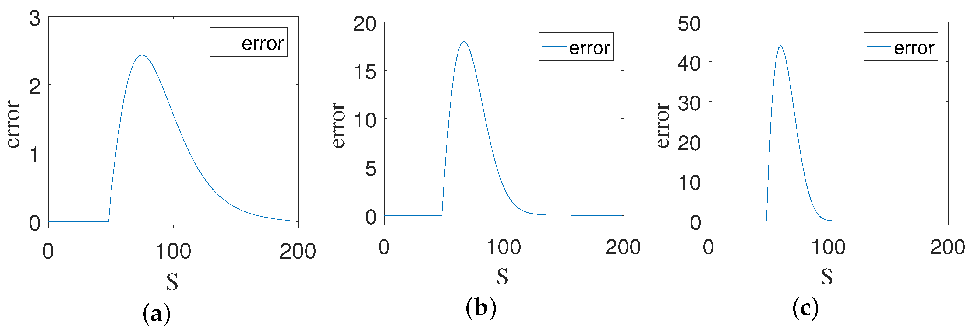
In Figure 1, we can obtain that whether the knock-in-barrier is triggered or not, the change of H value will affect the return of repayment. Therefore, we explore the relationship between the option price S and the return of repayment v and k v and the error between each other under a specific H value. Next, we take the specific H values of 0.3, 0.5, 0.7 and don’t change the values of other parameters. We get the figures of S and v, S and k v and figures of error between S and k v v . These figures are as shown below.
In Figure 2, Figure 3 and Figure 4, (a), (b), (c) in turn represent the result figures obtained when H values are 0.3, 0.5 and 0.7. In Figure 2 and Figure 3, we obtained that the change of v and k v with H is mainly in the range of S value from 50 to 100, which includes strike price and knock-in-barrier. With the increase of H value, the value of v and k v corresponding to S value on 50 to 100 will also increase. It can also be confirmed from Figure 4 that with the increase of H value, the maximum value of the error between v and k v also increases, and the range of the changed wave is about 50 to 100. Next, we explore whether the change of H value in different dimensions will also affect v and k v .

4.2. Two Underlying Assets

The same as one underlying asset, we first research the relationship between H x , H y and v as well as kv at a fixed point x , y under different values of H x and H y . We take values of H x and H y at equal intervals from 0.1 to 0.9 for 20 groups. We take n = 4 and take x and y from 0 to 300 for 31 groups. For other parameters, our values are as follow:
σ x = σ y = 0.3 , r = 0.03 , N x = N y = 30 , Δ x = Δ y = 10 , T = 1 , N t = 100 , Δ t = T N t = 0.01 ,
δ 1 = N t 4 , δ 2 = N t 2 , δ 3 = 3 N t 4 , δ 4 = N t + 2 , ρ x y = 0.5 , K 1 = 90 , K 2 = 85 , K 3 = 80 , K 4 = 75 ,
β 1 = 0.055 , β 2 = 0.11 , β 3 = 0.165 , β 4 = 0.22 , D = 50 , d = 0.16 .
K 1 to K 4 , β 1 to β 4 and δ 1 to δ 4 represent the strike price in strike date and the corresponding coupon rate. We can get the corresponding figures at a fixed point x , y = 100 , 100 as follows.
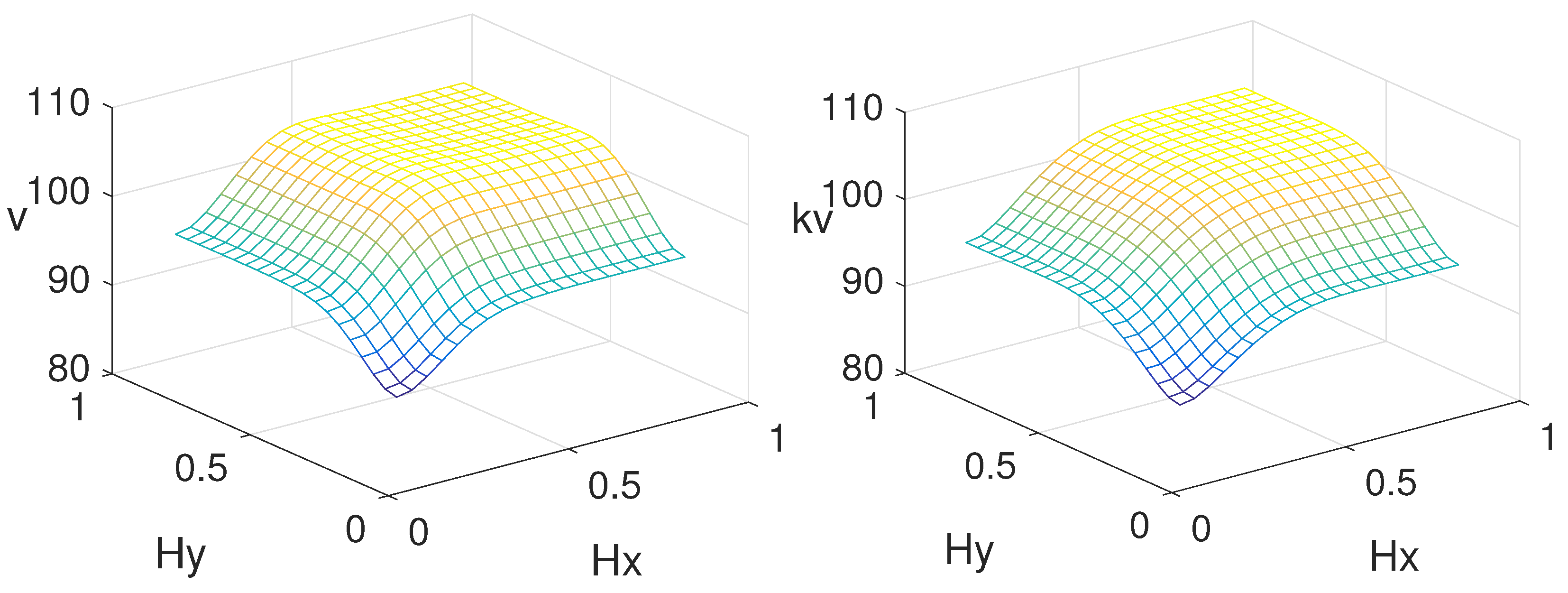
In Figure 5, we can observe that the change of H x , H y will also affect v and k v in the case of fixed point x , y . With the increase of H x and H y , the values of v and k v are also increasing. Therefore, we explore the relationship of x, y and v, x, y and k v . Next, we take the specific H x , H y values of 0.3, 0.5, 0.7 at the same time, and change N x = N y = 150 , Δ x = Δ y = 2 . We take x and y from 0 to 300 for 151 groups. Then, we don’t change the values of other parameters. We get the figures of x, y and v, x, y and k v . At the same time, we obtain the error figures of x, y and k v v . These figures are as shown in the Figure 6, Figure 7 and Figure 8 below.
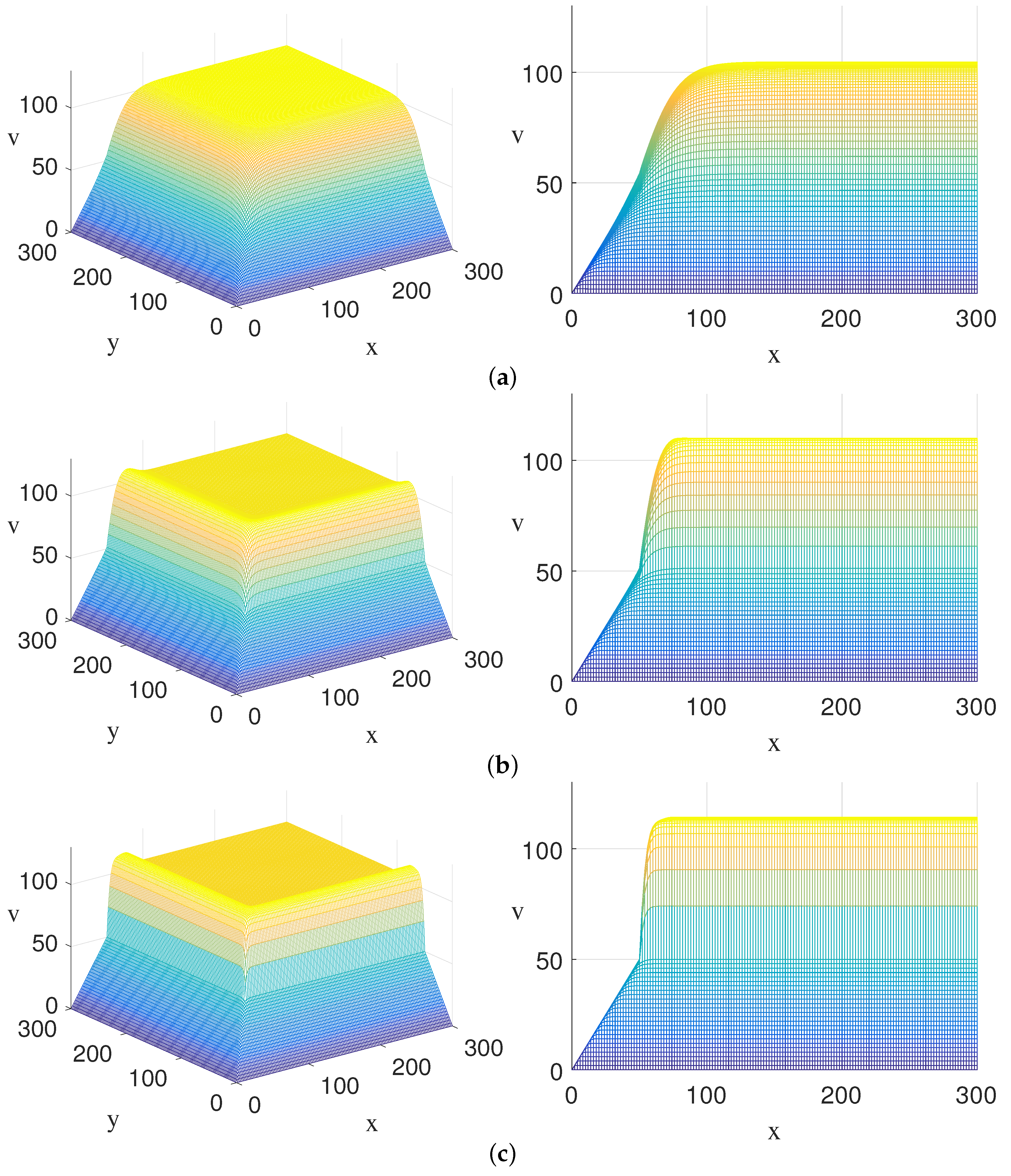
In Figure 6, Figure 7 and Figure 8, (a), (b), (c) in turn represent the result figures obtained when H x = H y = 0.3 , 0.5 , 0.7 . In Figure 6 and Figure 7, similar to the case of one asset, the change of H x and H y values will also affect the results of v and k v . The variation of v and k v values is mainly in the range of S value from 50 to 100, and this range just includes strike price and knock-in-barrier. If the influence of H x and H y on v and k v values is not considered in practical application, there will be a great error in calculating the return of repayment in the exercise stage, and even the result of wrong judgment. On the other hand, it can also be confirmed from Figure 8 that with the increase of H x and H y values, the maximum value of the error between v and kv also increases.

4.3. Three Underlying Assets

In three underlying assets, we also explore the relationship between H x , H y , H z and v as well as k v at a fixed point x , y , z and fixed value H z under different values of H x , H y . We take values of H x and H y at equal intervals from 0.1 to 0.9 for 20 groups. We take n = 4 and take x and y from 0 to 200 for 21 groups. For other parameters, our values are as follow:
σ x = σ y = σ z = 0.3 , r = 0.03 , N x = N y = N z = 20 , T = 3 , N t = 90 , Δ t = T N t = 1 30 ,
ρ x y = ρ y z = ρ x z = 0.5 , δ 1 = N t 6 , δ 2 = N t 3 , δ 3 = N t 2 , δ 4 = 4 N t 6 , δ 5 = 5 6 N t , δ 6 = 7 6 N t ,
K 1 = 95 , K 2 = 95 , K 3 = 90 , K 4 = 90 , K 5 = 85 , K 6 = 85 ,
β 1 = 0.05 , β 2 = 0.1 , β 3 = 0.15 , β 4 = 0.2 , β 5 = 0.25 , β 6 = 0.30 , D = 50 , d = 0.3
.
K 1 to K 4 , β 1 to β 4 and δ 1 to δ 4 represent the strike price in strike date and the corresponding coupon rate. We can get the corresponding figure at point x , y , z = 100 , 100 , 100 as follows.
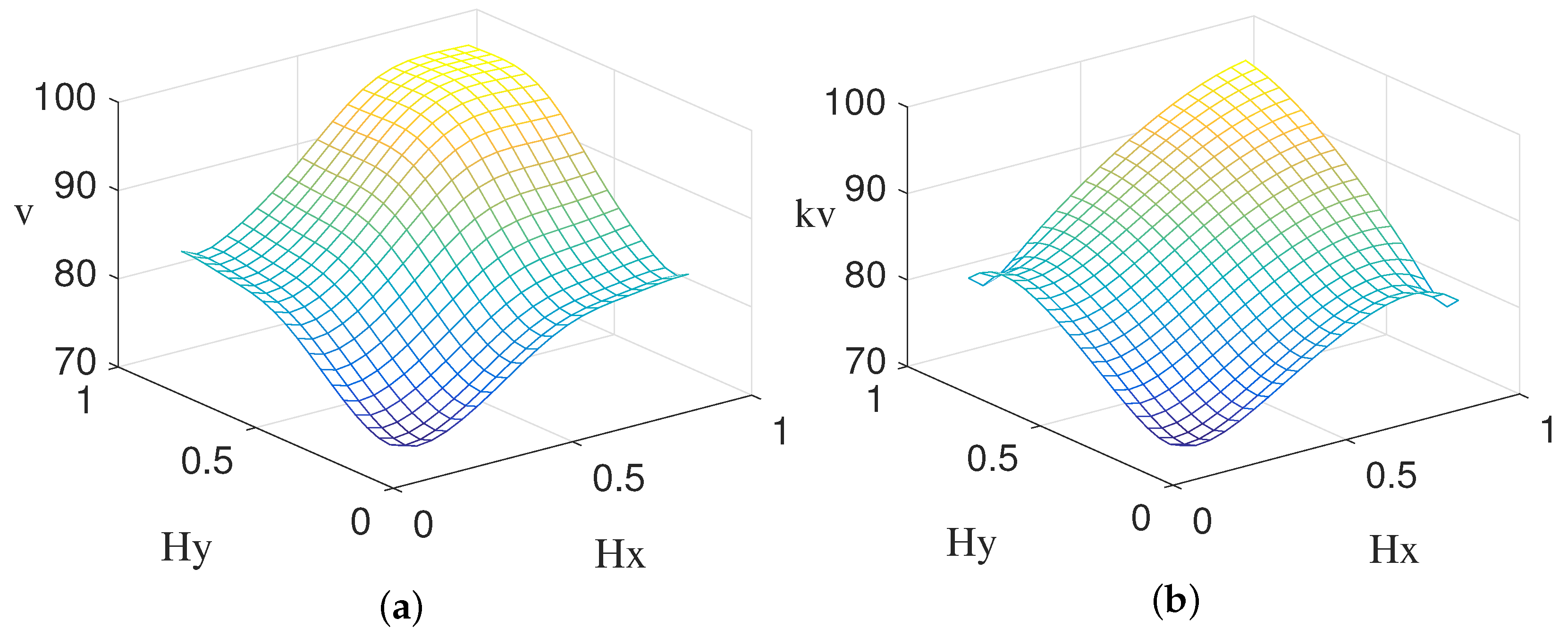
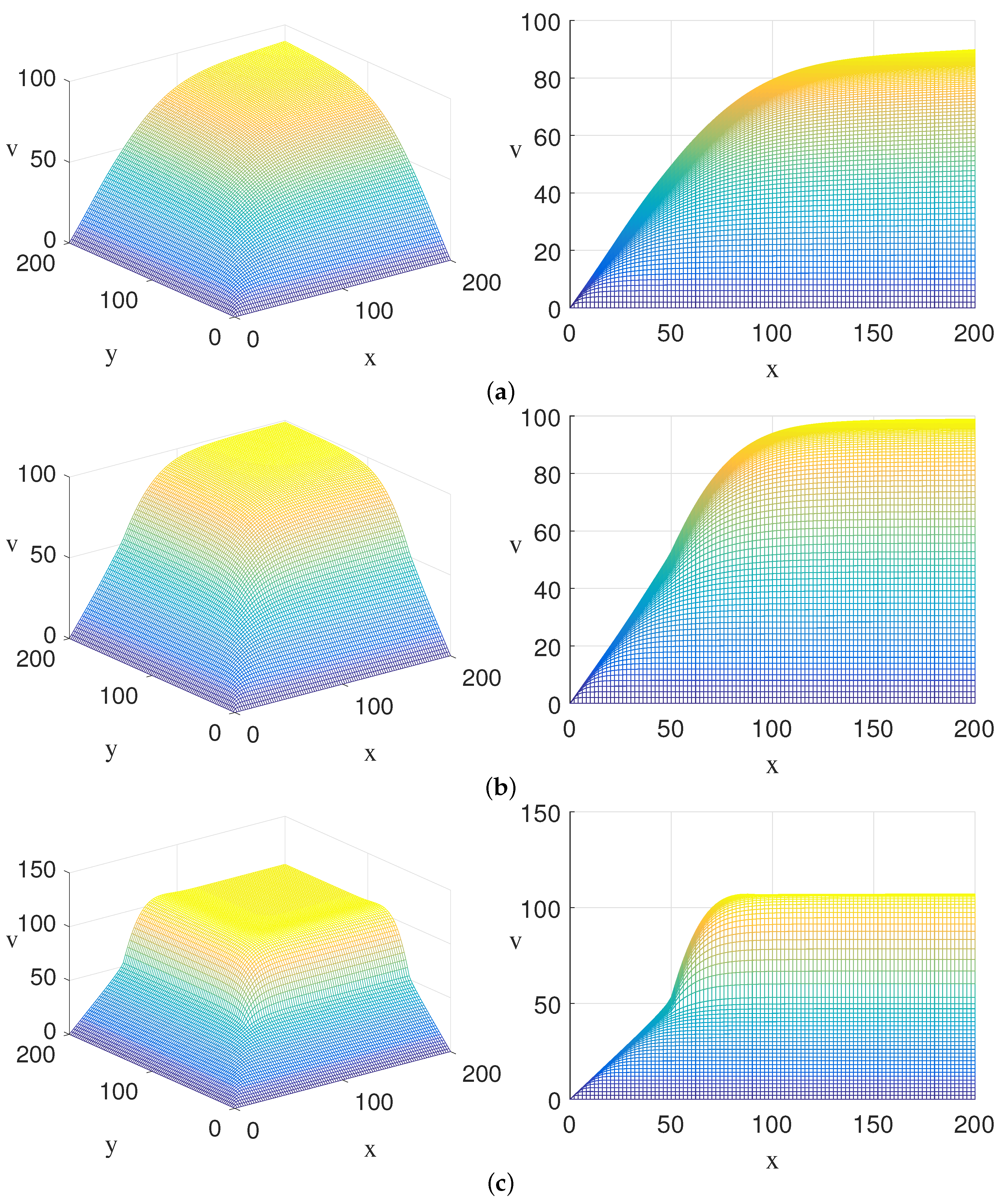
In Figure 9, (a) represents the figure of H x , H y and v at fixed point x , y , z = 100 , 100 , 100 when H z = 0.5 . (b) represents the figure of H x , H y and k v at fixed point x , y , z = 100 , 100 , 100 when H z = 0.5 . In two assets, we get the conclusion that the change of H x and H y will affect the results of v and k v . In three assets, this conclusion is still true, and with the increase of H x , H y values, the results of v and k v also increase. Next, we take the specific H x , H y , H z values of 0.3, 0.5, 0.7 at the same time, and change N x = N y = N z = 100 , Δ x = Δ y = Δ z = 2 . Therefore, we take x, y and z from 0 to 200 for 101 groups. And then we don’t change the values of other parameters. Therefore, we can get the figures of x, y and v, the figures of x, y and k v when z = 100 . At the same time, we also give the figures of x, y and k v v when z = 100 . These are as shown in Figure 10, Figure 11 and Figure 12 below.
In Figure 10, Figure 11 and Figure 12, (a), (b) and (c) respectively represent the corresponding figures when H x = H y = H z = 0.3 , 0.5 and 0.7 . In Figure 10 and Figure 11, we can observe the conclusion that the change of H value will still affect v and k v values, and the main change occurs in a reign containing strike price and knock-in-barrier. At the same time, we also calculate that v and k v at a fixed point x , y , z = 100 , 100 , 100 , when H x = H y = H z = 0.3 , the corresponding values of v and k v are 71.5396 and 89.7243 respectively. When H x = H y = H z = 0.5 , the corresponding values of v and k v at this point are 89.7243 and 84.2065. When H x = H y = H z = 0.7 , the corresponding values of v and k v at this point are 106.3668 and 95.9271. We can obtain that the value of v and k v increase with the increase of H x , H y and H z . In Figure 12, the error value increases with increase of H x , H y and H z values, which indicates that with the increase of H x , H y and H z values, the difference between v and k v value becomes significant. In practice, H value is not directly obtainable. Nowadays, the value of H is estimated mainly based on historical data. Barunik and Kristoufek [33] point out that it is most effective to estimate H by using the GHE method suitable for multifractal measurement of time series. But if the influence of H value is ignored, there may be a big error between the calculated result and the actual result, which will affect the final decision.

4.4. Empirical Evidence for Well-Posed of the Model and Validation of the Solution

In this section, we select an actual three-asset ELS product to price three-asset step-down ELS with Monte Carlo simulation )(MCs). The three-asset ELS product consists of three underlying assets such as KOSPI200, EU- ROSTOXX50, and S&P500 whose details can be accessed on 12 December 2020 and can be referred to website “http://www.miraeassetdaewoo.com”.
According to the investment statement of the selected ELS, we observe the following parameters as: the face value F = 10000 , the expiration time T = 3 , the volatilizes σ 1 = 0.2414 (KOSPI200), σ 2 = 0.2871 (EUROSTOXX50), σ 3 = 0.3509 (S&P500), the correlations of two underlying assets ρ 12 = 0.5474 , ρ 13 = 0.3357 , ρ 23 = 0.7172 , the dummy rate d = 0.135 , the initial prices of three-asset are 315.89 p t , 3160.95 p t , 3281.06 p t , which correspond to KOSPI200, EUROSTOXX50, and S&P500, respectively. Here for convenience, we set the benchmark prices of three underlying assets S ( 0 ) = S 1 ( 0 ) = S 2 ( 0 ) = S 3 ( 0 ) = 100 , then all the knock-in-barrier levels of three assets are D = 0.45 × S ( 0 ) . Besides, the free risk interest rate is chosen by the current London InterBank Offered Rate r = 0.023631 .
The next step is to determine the long-memory characteristics of each asset, namely, the values of Hurst exponent. There have been many methods proposed for estimating the Hurst exponent, we here adopt generalized Hurst exponent (GHE) approach to calculate the Hvalue of each asset. GHE is a suitable method for measuring the multifractality of time series. For instance, a time series S ( t ) with length N, where t = ( 1 , 2 , , δ t ) , calculate the H ( q ) based on the scaling of qth order moments defined by the distribution as K q ( τ ) = t = 0 N τ | X ( t + τ ) X ( t ) | q N τ + 1 , where 1 < τ < t m a x , and τ m a x always varies between 5 and 19, we choose τ m a x = 15 in this paper. We obtain the statistic scales by the power-law K q ( τ ) c τ q H ( q ) . When q = 2 , the K 2 ( τ ) represents the scaling of the auto-correlation function of the increments. We estimate the K 2 ( τ ) c τ 2 H ( 2 ) in this study, and we can easily estimate 2 H ( 2 ) by the least squares regression on logarithms of l o g K 2 ( τ ) and l o g τ , then we obtain the Hurst exponents for three-asset step-down ELS in the following table.
We observe from Table 2 that the classic ELS model calculates a price that is obviously higher than the reference price, whereas the proposed model almost exactly corresponds to the reference price. As a result, ELS models should take into consideration long-range correlations of underlying assets. Buyers or sellers will suffer significant losses when selling an ELS contract with large amounts, if not considering Hurst exponent. Besides, we average the 20 prices and obtain the ELS prices of the classical ELS model and the ELS-MCs model are 9109.8, and 8948.6 while the reference price is given by 8931.2.

4.5. Greeks

In one asset, we explore Greeks and obtain the conclusion that the change of H will affect the numerical solution of Greeks. Therefore, we also explore whether the change of H will also affect the numerical solution of three dimensional Greeks. We remain the value of parameters unchanged and use semi-implicit to obtain solution of Greeks in x direction. But in Rho, the value of r is selected in 0.02985 , 0.03015 . In Vega, the value of σ is selected in 0.3 , 0.4 . In x direction, we give the finite difference scheme of calculating Greeks.
Finite difference scheme of Greeks:
D e l t a = V x x , T V x + h , y , z , T V x h , y , z , T 2 h ,
G a m m a = V x x x , T V x h , y , z , T 2 V x , y , z , T + V x + h , y , z , T h 2 ,
T h e t a = V t x , T V x , y , z , T V x , y , z , T Δ t Δ t ,
R h o = V r x , T | r = 0.03 V x , y , z , T | r = 0.03015 V x , y , z , T | r = 0.02985 0.0003 ,
V e g a = V σ x x , T | σ x = 0.35 V x , y , z , T | σ x = 0.4 V x , y , z , T | σ x = 0.3 0.1 .
We also change the value of H x , H y , H z and we observe the numerical figures under different values of H x , H y , H z .
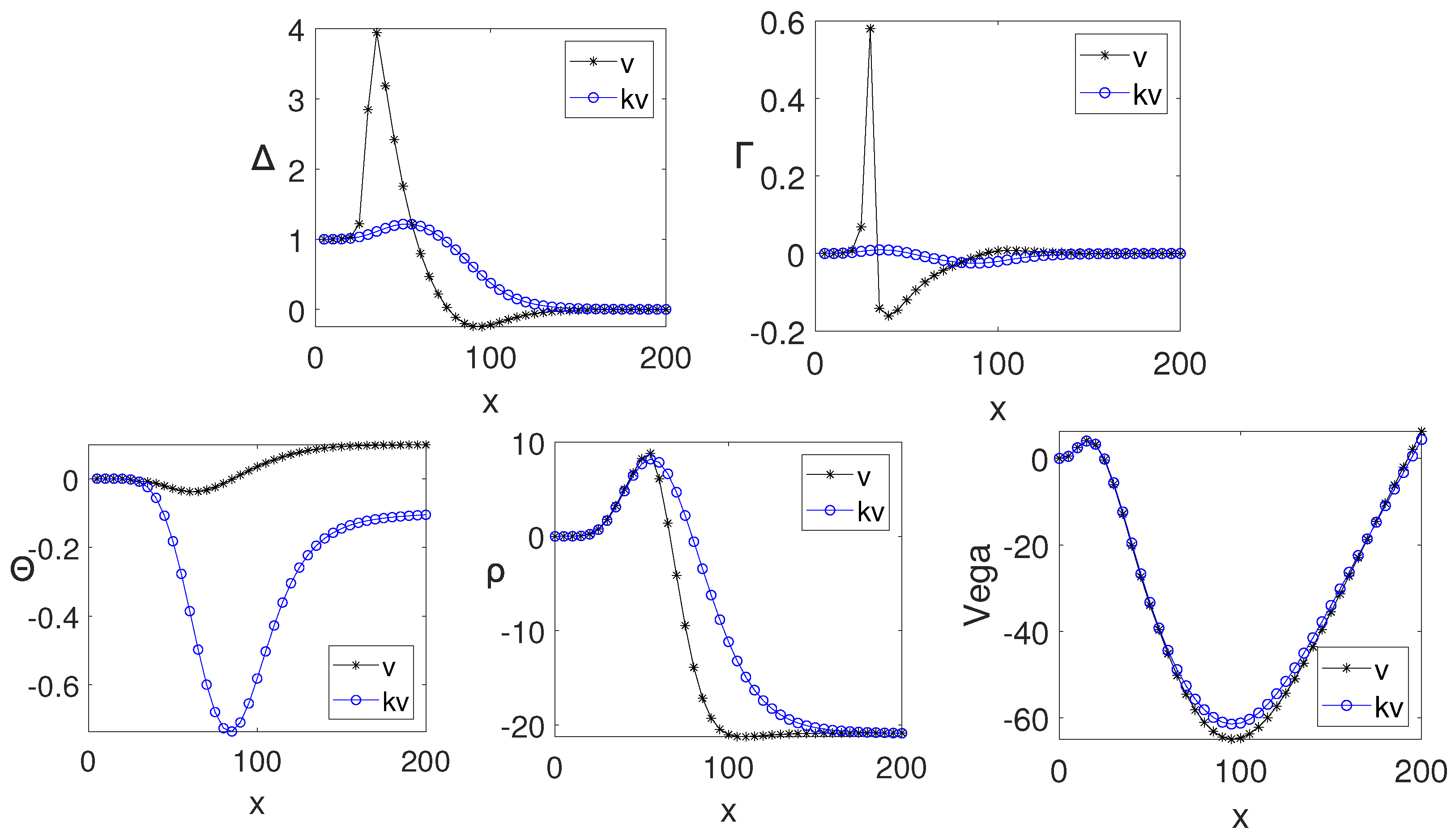
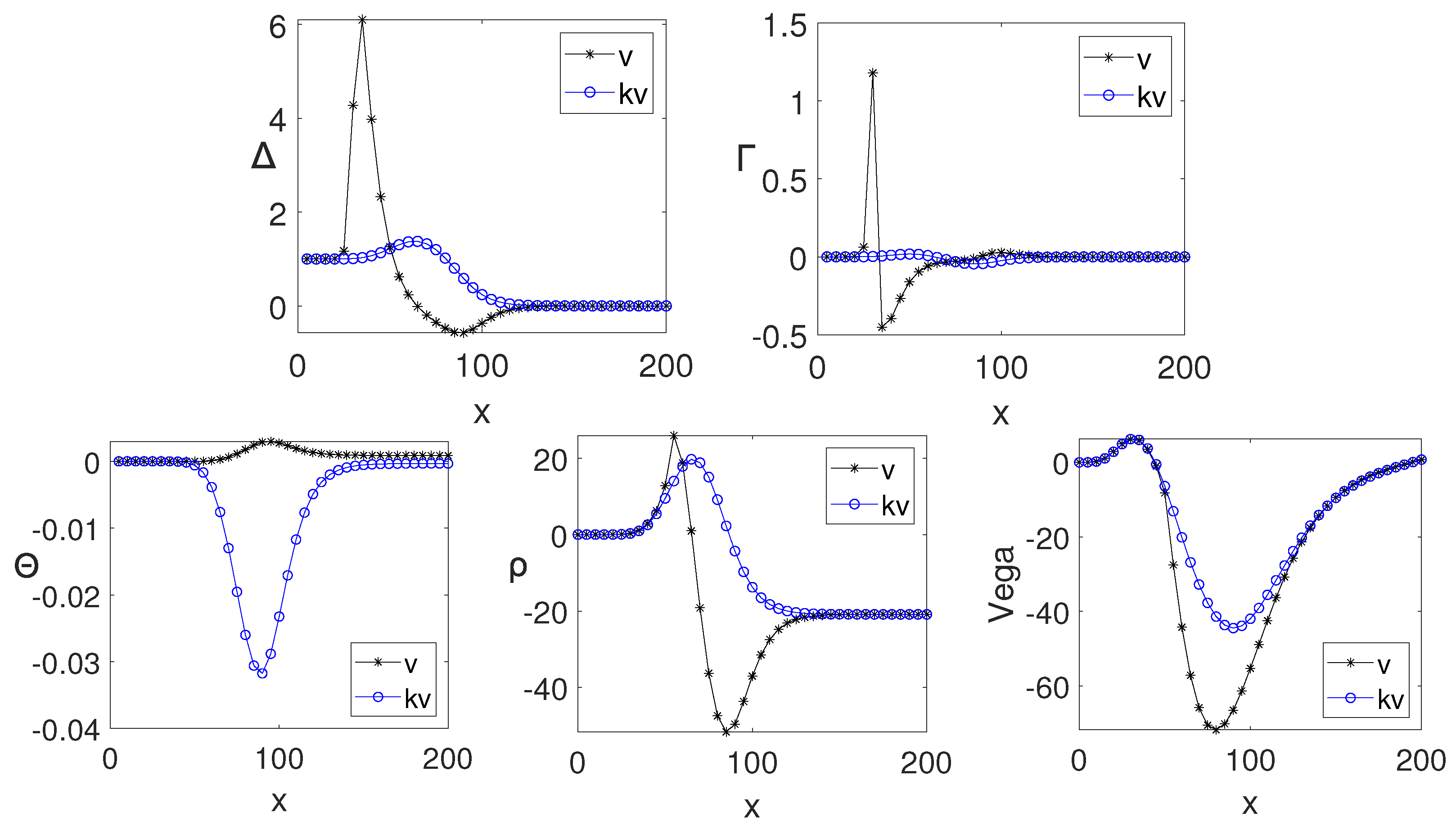
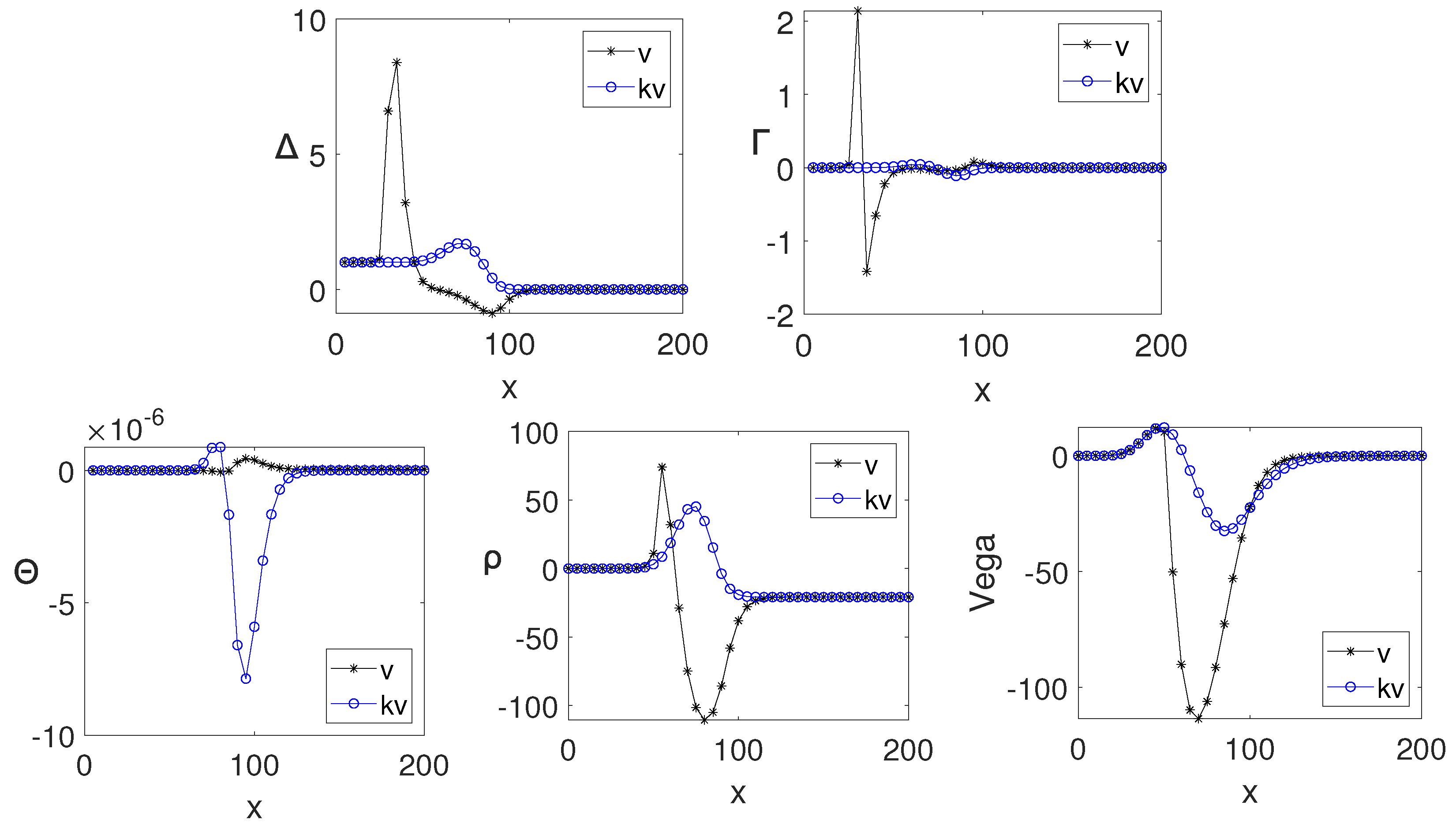
Delta is the rate of change of the option price with respect to the price of the underlying asset. With the increase of H x , H y , H z , the peak value of the figure increases gradually and the figure becomes steeper. Gamma is the change in the Delta of an option relative to the change in the underlying assets. With the increase of H x , H y , H z , the peak value of the figure also increases gradually and the figure also becomes steeper. Theta represents the speed of option yield decay with time. With the increase of H x , H y , H z , the value range of the curve in the figure fluctuates obviously. When H x = H y = H z = 0.7 , there are obvious fluctuations in this figure. Rho is the partial differential of option yield to risk-free interest rate. With the increase of H x , H y , H z , the peak value of the figure decline gradually. Vega is the ratio between the change of option price and the change of underlying asset volatility. With the increase of H x , H y , H z , the figure becomes smoother and wider. But the peak value of the figure hardly changed.
In Figure 13, Figure 14 and Figure 15, the black curve represents option price without knock-in-barrier and the blue curve stands for option price with knock-in-barrier. From the results of figures, we can obtain that the change of H will also affect the final result in the Greeks of three assets. In the fractional Black-Scholes model, there is a big error between the result and the actual result if we don’t consider the effect of H.
Our proposed model incorporates the concept of fractals on the basis of efficient market theory. Since the concept of fractal is added, there will be some changes in the price of options, which will lead to changes in Greeks. Considering that fractals add the historical volatility of stock prices into the calculation, this is consistent with the long-term memory, auto-correlation and persistence of stocks. More importantly, in the process of financial investment, considering the fractal exponents or not will have a considerable impact on investment Greeks risk hedging. When we consider the long-term correlation of stock prices, the fractal exponents helps us reduce the volatility of stock expectations which can effectively guide investment institutions or investors to reduce losses and increase revenue.

5. Conclusions

We established finite difference scheme for the step-down ELS option of one, two and three assets under the fractional Black-Scholes model. In the case of one asset, we established the Crank-Nicolson scheme, in the case of two assets, we established implicit scheme and in the case of three assets, we also used OSM method to establish semi-implicit scheme. Numerical experiments were performed after meshing at equal intervals, and the results were obtained. Regardless of whether the knock-in-barrier is triggered, the return of repayment will be affected by H. As the value of H increases, the return of repayment will also increase. The gap between the result v obtained when the knock-in-barrier is occurred and the result kv obtained when the knock-in-barrier is not occurred is also increasing. Under different assets forms, we also had explored the relationship between H and v and kv when option price is fixed. It can be confirmed that the conclusion that the values of v and kv increase with the increases of the value of H. We also conducted Greeks analysis and discovered that the values of Delta, Gamma, Theta, Rho and Vega are all different under the fractal exponents of 0.3, 0.5 and 0.7, which implies the stock price series of the investment market all have obvious long-term correlation and memory characteristics. In our model, during the process of hedging, different fractal exponents can provide investors or investment companies with constructive advice in the calculation process of Greeks hedging, and can help reduce losses in time before losses damage. Moreover, the option price can be more accurately described.

Author Contributions

Conceptualization, Software, Methodology X.W.; Writing-original draft, S.W.; Data curation, Validation, Visualization, W.S.; Writing—review & editing, Supervision, J.W. All authors have read and agreed to the published version of the manuscript.

Funding

This research was funded by the Natural Science Foundation of the Jiangsu Higher Education Institutions of China (Grant No. 22KJB110020).

Institutional Review Board Statement

Not applicable.

Informed Consent Statement

Not applicable.

Data Availability Statement

The data that support the findings of this study are available on request from the corresponding author upon reasonable request.

Acknowledgments

The corresponding author Jian Wang expresses thanks for the Natural Science Foundation of the Jiangsu Higher Education Institutions of China (Grant Nos. 22KJB110020). The authors are grateful to the reviewers for their valuable suggestions and comments, which significantly improved the quality of this article.

Conflicts of Interest

The authors declare no conflict of interest.

References

  1. Chen, A.H.; Kensinger, J.W. An analysis of market-index certificates of deposit. J. Financ. Serv. Res. 1990, 4, 93–110. [Google Scholar] [CrossRef]
  2. Baubonis, C.; Gastineau, G.L.; Purcell, D. The Banker’s Guide to Equity-Linked Certificates of Deposit. J. Deriv. 1993, 1, 87–95. [Google Scholar] [CrossRef]
  3. Kim, J.; Kim, T.; Jo, J.; Choi, Y.; Lee, S.; Hwang, H.; Yoo, M.; Jeong, D. A practical finite difference method for the three-dimensional Black-Scholes equation. Eur. J. Oper. Res. 2016, 252, 183–190. [Google Scholar] [CrossRef]
  4. Jeong, D.; Kim, J. A comparison study of ADI and operator splitting methods on option pricing models. J. Comput. Appl. Math. 2013, 247, 162–171. [Google Scholar] [CrossRef]
  5. Bachelier, L. Theoryofspeculation. In The Random Characterof Stock Market; Ksotner, P., Ed.; MIT Press: Cambridge, NA, USA, 1900. [Google Scholar]
  6. Sumuelson, P.A. Rational theory of warrant pricing. Ind. Manag. Rev. 1965, 6, 13–31. [Google Scholar]
  7. Black, F.; Scholes, M. The Pricing of Options and Corporate Liabilities. J. Political Econ. 1973, 81, 637–654. [Google Scholar] [CrossRef] [Green Version]
  8. Mandelbrot, B.B.; Van Ness, J.W. Fractional Brownian motion, fractional noises and applications. SIAM Rev. 1968, 10, 422–436. [Google Scholar] [CrossRef]
  9. Hazhir, A.; Mahsan, T.K.; Hamid, K. Option pricing under finite moment log stable process in a regulated market: A generalized fractional path integral formulation and Monte Carlo based simulation. Commun. Nonlinear Sci. Numer. Simul. 2020, 90, 105345. [Google Scholar]
  10. Lin, S.; He, J.X. A regime switching fractional Black–Scholes model and European option pricing. Commun. Nonlinear Sci. Numer. Simul. 2020, 85, 105222. [Google Scholar] [CrossRef]
  11. Grzegorz, K.; Marcin, M. A computational weighted finite difference method for American and barrier options in subdiffusive Black–Scholes model. Commun. Nonlinear Sci. Numer. Simul. 2021, 95, 105676. [Google Scholar]
  12. Peter, E.E. Fractal Structure in the Captial Market. Financ. Anal. J. 1989, 45, 32–37. [Google Scholar] [CrossRef]
  13. Karatzas, I.; Shreve, S.E. Brownian motion and stochastic calculus. Acta Appl. Math. 1991, 24, 197–200. [Google Scholar]
  14. Radu, V. Analysis of the Romanian Capital Market Using the Fractal Dimension. Fractal Fract. 2022, 6, 564. [Google Scholar] [CrossRef]
  15. Li, Y. Multifractal Characteristics of China’s Stock Market and Slump’s Fractal Prediction. Fractal Fract. 2022, 6, 499. [Google Scholar] [CrossRef]
  16. Zhang, J.; Wang, Y.; Zhang, S. A New Homotopy Transformation Method for Solving the Fuzzy Fractional Black–Scholes European Option Pricing Equations under the Concept of Granular Differentiability. Fractal Fract. 2020, 6, 286. [Google Scholar] [CrossRef]
  17. Sarraj, M.; Ben Mabrouk, A. The Systematic Risk at the Crisis—A Multifractal Non-Uniform Wavelet Systematic Risk Estimation. Fractal Fract. 2021, 5, 135. [Google Scholar] [CrossRef]
  18. Necula, C. Option Pricing in a Fractional Brownina Motion Environment. Math. Rep. 2002, 2, 259–273. [Google Scholar]
  19. Liu, S.Y.; Yang, X.Q. Pricing of european option on dividend-paying stock in a fractional Brownian motion environment. Math. Econ. 2002, 19, 35–39. [Google Scholar]
  20. Murwaningtyas, C.E.; Kartiko, S.H.; Gunardi Suryawan, P.H. European option pricing by using a mixed fractional brownian motion. J. Phys. Conf. Ser. 2019, 1180, 012081. [Google Scholar] [CrossRef]
  21. Wang, J.; Yan, Y.; Chen, W.B.; Shao, W.; Tang, W.W. Equitylinked securities option pricing by fractional brownian motion. Chaos Solitons Fractals 2021, 144, 110716. [Google Scholar] [CrossRef]
  22. Ali, A.; Abbas, M.; Akram, T. New group iterative schemes for solving the two-dimensional anomalous fractional sub-diffusion equation. J. Math. Comp. Sci. 2021, 22, 119–127. [Google Scholar] [CrossRef]
  23. Oderinu, R.A.; Owolabi, J.A.; Taiwo, M. Approximate solutions of linear time-fractional differential equations. J. Math. Comput. Sci. 2023, 29, 60–72. [Google Scholar] [CrossRef]
  24. Nikan, O.; Golbabai, A.; Machado, J.A.; Nikazad, T. Numerical solution of the fractional Rayleigh–Stokes model arising in a heated generalized second-grade fluid. Eng. Comput. 2021, 37, 1751–1764. [Google Scholar] [CrossRef]
  25. Golbabai, A.; Ahmadian, D.; Milev, M. Radial basis functions with application to finance: American put option under jump diffusion. Math. Comput. Model. 2012, 55, 1354–1362. [Google Scholar] [CrossRef]
  26. Golbabai, A.; Nikan, O.; Nikazad, T. Numerical investigation of the time fractional mobile-immobile advection-dispersion model arising from solute transport in porous media. Int. J. Appl. Comput. Math. 2019, 5, 1–22. [Google Scholar] [CrossRef]
  27. Golbabai, A.; Nikan, O. A computational method based on the moving least-squares approach for pricing double barrier options in a time-fractional Black–Scholes model. Comput. Econ. 2020, 55, 119–141. [Google Scholar] [CrossRef]
  28. Golbabai, A.; Nikan, O.; Nikazad, T. Numerical analysis of time fractional Black–Scholes European option pricing model arising in financial market. Comput. Appl. Math. 2019, 38, 1–24. [Google Scholar] [CrossRef]
  29. Nikan, O.; Avazzadeh, Z.; Tenreiro Machado, J.A. Localized kernel-based meshless method for pricing financial options underlying fractal transmission system. Mathematical Methods in the Applied Sciences. Math. Methods Appl. Sci. 2021. [Google Scholar] [CrossRef]
  30. Hu, Y.; Oksendal, B. Fractional white noise calculus and applications to finance. In Infinite Dimensional Analysis Quantum Probability and Related Topics; World Scientific: Singapore, 2003; Volume 6(01), pp. 1–32. [Google Scholar]
  31. Duffy, D.J. Finite Difference Methods in Financial Engineering: A Partial Differential Equation Approach, 2nd ed.; John Wiley and Sons: New York, NY, USA, 2006. [Google Scholar]
  32. Jeong, D.; Wee, I.S.; Kim, J. An operator splitting method for pricing the ELS option. J. Korean Soc. Ind. Appl. Math. 2010, 14, 175–187. [Google Scholar]
  33. Barunik, J.; Kristoufek, L. On Hurst exponent estimation under heavy-tailed distributions. Phys. A 2010, 389, 3844–3855. [Google Scholar] [CrossRef]
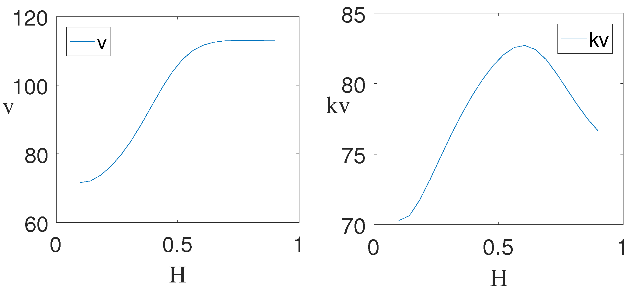
Figure 1. The effect of different H on v and k v when S = 70 .
Fractalfract 07 00126 g001
Figure 2. (a) denotes v for different S when H = 0.3 , (b) denotes v for different S when H = 0.5 and (c) denotes v for different S when H = 0.7 .
Fractalfract 07 00126 g002
Figure 3. (a) denotes k v for different S when H = 0.3 , (b) denotes k v for different S when H = 0.5 and (c) denotes k v for different S when H = 0.7 .
Fractalfract 07 00126 g003
Figure 4. (a) denotes k v v for different S when H = 0.3 , (b) denotes k v v for different S when H = 0.5 and (c) denotes k v v for different S when H = 0.7 .
Fractalfract 07 00126 g004
Figure 5. The effect of different H x and H y on v and k v when x , y = 100 , 100 .
Fractalfract 07 00126 g005
Figure 6. (a) denotes v for different x, y when H x = H y = 0.3 , (b) denotes v for different x, y when H x = H y = 0.5 and (c) denotes v for different x, y when H x = H y = 0.7 .
Fractalfract 07 00126 g006
Figure 7. (a) denotes k v for different x, y when H x = H y = 0.3 , (b) denotes k v for different x, y when H x = H y = 0.5 and (c) denotes k v for different x, y when H x = H y = 0.7 .
Fractalfract 07 00126 g007
Figure 8. (a) denotes k v v for different x, y when H x = H y = 0.3 , (b) denotes k v v for different x, y when H x = H y = 0.5 and (c) denotes k v v for different x, y when H x = H y = 0.7 .
Fractalfract 07 00126 g008
Figure 9. The effect of different H x , H y on v and k v when x , y , z = 100 , 100 , 100 and H z = 0.5 .
Fractalfract 07 00126 g009
Figure 10. (a) denotes v for different x, y when H x = H y = H z = 0.3 and z = 100 , (b) denotes v for different x, y when H x = H y = H z = 0.5 and z = 100 and (c) denotes v for different x, y when H x = H y = H z = 0.7 and z = 100 .
Fractalfract 07 00126 g010
Figure 11. (a) denotes k v for different x, y when H x = H y = H z = 0.3 and z = 100 , (b) denotes k v for different x, y when H x = H y = H z = 0.5 and z = 100 and (c) denotes k v for different x, y when H x = H y = H z = 0.7 and z = 100 .
Fractalfract 07 00126 g011
Figure 12. (a) denotes k v v for different x, y when H x = H y = H z = 0.3 and z = 100 , (b) denotes k v v for different x, y when H x = H y = H z = 0.5 and z = 100 and (c) denotes k v v for different x, y when H x = H y = H z = 0.7 and z = 100 .
Fractalfract 07 00126 g012
Figure 13. H x = H y = H z = 0.3 , figures represent in turn are Delta, Gamma, Theta, Rho and Vega. The blue curve stands for option price with knock-in-barrier while the black curve represents option price without knock-in-barrier. For interpretation of the references to color in the figure, the reader is referred to the web version of the article.
Fractalfract 07 00126 g013
Figure 14. H x = H y = H z = 0.5 , figures represent in turn are Delta, Gamma, Theta, Rho and Vega. The blue curve stands for option price with knock-in-barrier while the black curve represents option price without knock-in-barrier. For interpretation of the references to color in the figure, the reader is referred to the web version of the article.
Fractalfract 07 00126 g014
Figure 15. H x = H y = H z = 0.7 , figures represent in turn are Delta, Gamma, Theta, Rho and Vega. The blue curve stands for option price with knock-in-barrier while the black curve represents option price without knock-in-barrier. For interpretation of the references to color in the figure, the reader is referred to the web version of the article.
Fractalfract 07 00126 g015
Table 1. Parasmeters of fractional step-down ELS.
Hurst ExponentStrike PriceUnderlying Asset Price
HKS
MaturityKnock-in-barrierDummy
TDd
Numer of observation datesFace valueStrike date
nF δ
VolatilityRisk-free rateCoupon rate
σ r β
Table 2. Hurst exponents for three-asset step-down ELS calculated by GHE approach.
KOSPI200EUROSTOXX50S&P500
H 1 H 2 H 3
0.49460.49410.4870
Disclaimer/Publisher’s Note: The statements, opinions and data contained in all publications are solely those of the individual author(s) and contributor(s) and not of MDPI and/or the editor(s). MDPI and/or the editor(s) disclaim responsibility for any injury to people or property resulting from any ideas, methods, instructions or products referred to in the content.