An Analysis of the Effects of Lifestyle Changes by Using a Fractional-Order Population Model of the Overweight/Obese Diabetic Population

Abstract

Unbalanced lifestyles and other underlying medical conditions are responsible for the worrying pace at which diabetes mellitus is becoming a global health crisis. Recent studies suggest that placing a diabetic patient into remission through a rigorous lifestyle change program can normalize blood glucose levels. This research focuses on fractional order derivative-based mathematical modeling and analysis of the diabetes mellitus model with remission parameters. Firstly, the existence and uniqueness of the solution of the diabetes mellitus model are discussed. Non-negativity and boundedness are also examined. Afterward, the concept of the Jacobian matrix is used to investigate the stability of the model’s equilibrium points. The Daftardar-Gejji and Jafari Method has finally been applied to approximate the solutions. The conclusions drawn from numerical simulations of the diabetic model with fractional-order derivatives show a clear dependence on the remission parameters and fractional-order derivative.

1. Introduction

Diabetes mellitus is a chronic disease that develops when the pancreas either fails to create enough insulin, the body cannot utilize insulin effectively, or the pancreas fails to make insulin entirely. The blood sugar regulation hormone, insulin, is essential for preserving the appropriate blood sugar level. One of the most common complications of untreated diabetes is elevated blood glucose levels, which occur when there is a problem with insulin hormone release. Diabetes is becoming a serious public health issue that poses a significant financial and social burden on every nation. Generally, diabetes falls into two types.

• When $\beta$—cells that synthesize and release insulin and amylin in pancreatic islets become extinct, it results in type 1 diabetes, which is also known as insulin-dependent diabetes (IDD), which is characterized by insufficient insulin production and hyperglycemia.
• Type 2 diabetes, also known as non-insulin-dependent diabetes (NIDD), has a variety of causes, with heredity and lifestyle being two of the most crucial causes.

The World Health Organization (WHO) and the International Diabetes Federation (IDF) are institutions that gather data and develop diabetes policies on a global scale. The most recent reports from the WHO [1] and the IDF [2,3] raise concerns. Age-specific diabetes mortality rates increased by 3% between 2000 and 2019. In 2019, diabetes and kidney disease associated with diabetes were estimated to cause 2 million deaths. The direct cause of 1.5 million deaths in 2019 was diabetes, and 48% of these deaths occurred in people under the age of 70 years. Elevated blood glucose is responsible for 20% of cardiovascular mortality, and diabetes contributes to a further 460,000 deaths from kidney disease [4]. The IDF recently released data for 2021, indicating that 6.7 million deaths, or one death every five seconds, were attributable to diabetes [2,3]. Additionally, by 2045, this figure is projected to reach 784 million [2].

More than 80% of all type 2 diabetes cases are correlated with lifestyles that lead to overweight and obesity [5]. With so many children and teenagers currently overweight or obese, an increase in diabetes among younger individuals is predicted. Dietary factors causing an excess of calories to be deposited as body fat are the primary cause of obesity. Sedentary behavior and lack of physical activity result in fewer calories being burned off, leading to an increase in body weight. One way healthcare providers and legislators can collaborate to improve diabetes prevention efforts is by focusing on the diabetic population. For years, researchers have been attracted to studying population-based diabetic models. Boutayeb et al. [6] developed the first diabetic population framework using ordinary differential equations as follows:

$$\left\{\begin{array}{c}\begin{array}{cc}\hfill \frac{dD\left(t\right)}{dt}& =I-(\alpha +\omega )D\left(t\right)+\varsigma C\left(t\right)\hfill \\ \hfill \frac{dC\left(t\right)}{dt}& =\alpha D\left(t\right)-(\varsigma +\omega +\vartheta +\theta )C\left(t\right),\hfill \end{array}\hfill \end{array}\right.$$

(1)

where D represents the number of individuals with diabetes with no complications, C represents the number of diabetic individuals with complications, I stands for the incidence of diabetics with the assumption that there are no complications at this stage, $\alpha$ represents the rate at which complications develop, $\varsigma$ represents the complication recovery rate, $\vartheta$ represents the rate at which complications caused by diabetes lead to fatalities, and $\theta$ represents the rate at which C experiences permanent disability. The (1) structure has since been formulated into multiple research models that consider other aspects, including prediabetic and healthy people, awareness campaigns, genetics, and lifestyle and social influences.

In recent research, type II diabetes has been taken into account. Sweatman and Hassell [7] provided a framework for obtaining time-based health and sickness courses and examined the impact of changing the CHO and fat content of the diet on these time courses. A mathematical framework describing the endocrine glucose–insulin metabolic regulation feedback loop was put forth by Al-Hussein et al. [8], and its numerical investigation was provided. Kouidere et al. have developed a mathematical approach for the optimal regulation of diabetes mellitus [9]. They implemented four controllers in the model system, including treatment, psychological support, and awareness campaigns through media and education. By considering the impact of general public knowledge about diabetes mellitus in deterministic and stochastic situations, Mollah et al. created mathematical models [10]. Their findings demonstrated that a public awareness campaign could reduce the prevalence of diabetes mellitus. Additionally, Mollah et al. created a model centered on interactions between the density of diabetes awareness programs and the number of diabetic patients [11].

Several dynamical structures are modeled in fractional order instead of integer order because of the effect of memory or a non-local aspect. Additionally, fractional-order differential equations (FDEs) are thought to be incredibly reliable and precise. With the additional degree of freedom that fractional derivative offers, the real system or phenomena occurring in daily life (individuals with diabetes and their recovery) can be accurately approximated while employing fewer modeling parameters [12]. This is clear from [13], where the authors replaced several parameters with fractional derivatives and obtained findings that were reasonably accurate to the data. The fractional-order products are also utilized to broaden the system’s stability zone. By using two immune effectors, Ahmed et al. established a fractional-order cancer model [14]. They noted that the order of fractional derivatives controlled the system’s behavior. The same model with an RL derivative was also studied by Srivastava et al., who solved it using the homotopy decomposition method [15]. The population model of diabetes of healthy individuals, overweight/obese people, and diabetics with and without complications in Morocco was modeled in 2022 by Mohamed Lamlili E.N. et al. [16].

$$\left\{\begin{array}{c}\begin{array}{cc}\hfill \frac{dP\left(t\right)}{dt}& =\eta -\left(\epsilon +{\delta }_1+{\varpi }_1+\theta \right)P+{\varpi }_{2}W\hfill \\ \hfill \frac{dW\left(t\right)}{dt}& ={\varpi }_{1}P-\left({\varpi }_2+{\varpi }_3+{\varpi }_4+\theta \right)W\hfill \\ \hfill \frac{dD\left(t\right)}{dt}& ={\delta }_{1}P+{\varpi }_{3}W-\left({\delta }_2+\theta \right)D\hfill \\ \hfill \frac{dC\left(t\right)}{dt}& =\epsilon P+{\varpi }_{4}W+{\delta }_{2}D-\left(\theta +\nu \right)C,\hfill \end{array}\hfill \end{array}\right.$$

(2)

where $P\left(t\right)$—Population of adults without diabetes and overweight;

• $W\left(t\right)$—Population of overweight/obese adults;
• $D\left(t\right)$—Adult population of diabetics without complications;
• $C\left(t\right)$—Adult population of diabetics with complications;
• $\eta$—The prevalence of the population of adults;
• $\epsilon$—The frequency of healthy people suffering from difficulties;
• ${\delta }_1$—The rate at which healthy people develop diabetes;
• ${\delta }_2$—The frequency of complications emerging in persons with diabetes;
• ${\varpi }_1$—The ratio of healthy people who become overweight or obese;
• ${\varpi }_2$—The ratio of overweight or obese people who become healthy;
• ${\varpi }_3$—The ratio of overweight or obese people who become diabetic;
• ${\varpi }_4$—The ratio of overweight or obese people who develop complications;
• $\theta$—The rate of natural mortality;
• $\nu$—The mortality rate due to complications.

They found that educating policymakers about a healthy lifestyle, which includes consuming nutritious food, engaging in physical activity, and maintaining a suitable weight, is the most effective technique for reducing their risk of becoming overweight or obese.

Since fractional order derivatives can provide greater accuracy with actual world occurrences compared to integral order derivatives and have the property of historical memory, this study expands the concept and utilizes fractional order derivatives in the diabetes population model [16]. Moreover, we incorporated remission parameters into the population model to eliminate individuals with diabetes who consistently lead healthy lives. The diabetic mellitus population model with overweight/obesity has not been analyzed using fractional order derivatives so far. The presented study emphasizes the effect on the diabetic mellitus population model when a fractional order derivative is used. We incorporate two additional characteristics into the framework of the diabetic population model. We aim to illustrate the impact of adopting a healthy lifestyle (a style of life that incorporates nutritious food, regular exercise, meditation, and other healthy practices into everyday routines to reduce the chance of becoming seriously ill or dying prematurely) on remission. We then examine the impact of the fractional order $\sigma$ derivative on the model of the population with diabetes regardless of a remission parameter.

Therefore, the proposed model is defined as

$$\begin{array}{cc}\hfill {}^C{D}_0^{\sigma }A\left(t\right)& =\eta -\left({\alpha }_1+{\beta }_1+r_1+\mathsf{\mu }\right)A\left(t\right)+{\alpha }_{3}I\left(t\right),\hfill \\ \hfill {}^C{D}_0^{\sigma }I\left(t\right)& ={\alpha }_{1}A\left(t\right)-({\alpha }_2+{\alpha }_3+{\alpha }_4+\mathsf{\mu })I\left(t\right),\hfill \\ \hfill {}^C{D}_0^{\sigma }D\left(t\right)& ={\beta }_{1}A\left(t\right)+{\alpha }_{2}I\left(t\right)-({\beta }_2+r_2+\mathsf{\mu })D\left(t\right),\hfill \\ \hfill {}^C{D}_0^{\sigma }C\left(t\right)& ={\alpha }_{4}I\left(t\right)+{\beta }_{2}D\left(t\right)-(\delta +\mathsf{\mu })C\left(t\right),\hfill \end{array}$$

(3)

where $A\left(t\right)$—Number of people following a healthy lifestyle (not overweight/obese) on a regular basis;

• $I\left(t\right)$—Number of people not following a healthy lifestyle ( overweight/obese) on a regular basis;
• $D\left(t\right)$—Number of people with diabetes without any complication;
• $C\left(t\right)$—Number of people with diabetes with complications;
• $N\left(t\right)=A\left(t\right)+I\left(t\right)+D\left(t\right)+C\left(t\right)$
• $\eta$—The prevalence of the population;
• ${\alpha }_1$—The rate at which individuals following a healthy lifestyle are unable to maintain it regularly and become obese;
• ${\alpha }_2$—The ratio of obese people who do not follow a healthy lifestyle regularly and become diabetic;
• ${\alpha }_3$—The rate at which individuals following a healthy lifestyle are able to control obesity;
• ${\alpha }_4$—The ratio of obese/overweight people who do not follow a healthy lifestyle and develop diabetes with complications;
• ${\beta }_1$— The rate at which people following a healthy lifestyle on a daily basis develop diabetes without complications;
• ${\beta }_2$— The frequency of complications emerging in persons with diabetes; $\mathsf{\mu }$—The rate of natural mortality;
• $\delta$—The rate at which diabetics with complications die or are removed due to permanent disability;
• $r_1$—The probability rate at which people following a healthy lifestyle go into the remission category can be seen as the rate at which pre-diabetic individuals do not become diabetic by adopting a healthy lifestyle;
• $r_2$—The probability rate at which diabetic patients without complications fall into the remission category by regularly applying a healthy lifestyle.

Sections of this article are divided as follows: In Section 2, preliminaries and notations that are used throughout this work are provided. Existence and uniqueness, non-negativity and boundedness, and the identification and stability analysis of equilibrium points for the provided model are discussed in Section 3. Section 4 presents the approximate solution and graphical interpretation. Finally, the conclusion of this work is provided in Section 5.

2. Preliminaries and Notations

Definition 1. 

Let $\xi \left(z\right)\in C[a,b],a<z<b$ be a real-valued function, then for any $\sigma \in R^{+}$, the Riemann–Liouville fractional integral of order σ for the function $\xi \left(z\right)$, stated as

$${\mathrm{I}}_a^{\sigma }\xi \left(z\right)=\frac{1}{\mathsf{\Gamma }\left(\sigma \right)}\underset{a}{\overset{z}{\int }}{\left(z-\mathsf{\mu }\right)}^{\sigma }\xi \left(\mathsf{\mu }\right)d\mathsf{\mu },z>a.$$

• For $\sigma =0$, the integral is called the identity operator as ${\mathrm{I}}_a^0\xi \left(z\right)=\xi \left(z\right).$
• Unless specified, we will use $a=0.$
• The integral for the power function is defined as

  $${\mathrm{I}}_a^{\sigma }{(z-\alpha )}^{\omega }=\frac{\mathsf{\Gamma }(\omega +1)}{\mathsf{\Gamma }(\omega +\sigma +1)}{(z-\alpha )}^{\omega +\sigma },\omega >-1.$$

Definition 2. 

Let $\xi \left(z\right)\in C[a,b],a<z<b$ be a real-valued function. Then, for any $\sigma \in R^{+}$, the Riemann–Liouville fractional derivative of order σ for the function $\xi \left(z\right)$ is defined as

$$\begin{array}{c}{}^{RL}{D}_a^{\sigma }\xi \left(z\right)=\frac{d^k}{d{z}^k}\left({\mathrm{I}}_a^{k-\sigma }\xi \left(z\right)\right),k-1<\sigma \le k.\hfill \\ =\left\{\begin{array}{c}\frac{1}{\mathsf{\Gamma }(k-\sigma )}\frac{d^k}{d{z}^k}\left(\underset{a}{\overset{z}{\int }}{\left(z-\mathsf{\mu }\right)}^{k-\sigma -1}\xi \left(\mathsf{\mu }\right)d\mathsf{\mu }\right),k-1<\sigma <k\hfill \\ \frac{d^k}{d{z}^k}\xi \left(z\right),k=\sigma \hfill \end{array}\right\},\hfill \end{array}$$

• The Riemann–Liouville fractional derivative of the constant is

  $${}^{RL}{D}_a^{\sigma }Const=\frac{z^{\sigma }}{\mathsf{\Gamma }(1-\sigma )}Const\ne 0.$$
• The Riemann–Liouville σ order fractional derivative for the power function is defined as

  $${}^{RL}{D}_a^{\sigma }{(z-\alpha )}^{\omega }=\frac{\mathsf{\Gamma }(\omega +1)}{\mathsf{\Gamma }(\omega -\sigma +1)}{(z-\alpha )}^{\omega -\sigma },\omega >-1.$$

Definition 3. 

Let $\xi \left(z\right)\in C^k[a,b],a<z<b$ be a real-valued function. Then, for any $\sigma \in R^{+}$, the Caputo fractional σ order derivative for function $\xi \left(z\right)$ is stated as

$$\begin{array}{c}{}^C{D}_a^{\sigma }\xi \left(z\right)=I_a^{k-\sigma }\left(\frac{d^k}{d{z}^k}\xi \left(z\right)\right),k-1<\sigma \le k.\hfill \\ =\left\{\begin{array}{c}\frac{1}{\mathsf{\Gamma }(k-\sigma )}\left(\underset{a}{\overset{z}{\int }}{\left(z-\mathsf{\mu }\right)}^{k-\sigma -1}\left(\frac{d^k}{d{z}^k}\xi \left(\mathsf{\mu }\right)\right)d\mathsf{\mu }\right),k-1<\sigma <k\hfill \\ \frac{d^k}{d{z}^k}\xi \left(z\right),k=\sigma \hfill \end{array}\right\}.\hfill \end{array}$$

Remark 1. 

The Caputo fractional derivative for the power function is defined as

$${}^C{D}_a^{\sigma }{(z-\alpha )}^{\omega }=\frac{\mathsf{\Gamma }(\omega +1)}{\mathsf{\Gamma }(\omega -\sigma +1)}{(z-\alpha )}^{\omega -\sigma },\omega >k-1,k-1<\sigma \le k.$$

(4)

Definition 4. 

Let $f(t,X):[t_0,\infty )\times \mathsf{\Omega }\to R^n,\mathsf{\Omega }\subseteq R^n$ be a real-valued continuous function. Then, $f(t,X)$ is said to satisfy the Lipschitz condition, with respect to X, if there exists a positive real number L, such that

$$\left|f(t,X_1)-f(t,X_2)\right|\le L\left|X_1-X_2\right|,$$

for $X_1,X_2\in \mathsf{\Omega }\subseteq R^n$

Lemma 1. 

By using [17], for the fractional differential system

$${}^C{D}_0^{\sigma }X\left(t\right)=f(t,X),t>t_0,X\left(t_0\right)>0,\sigma \in (0,1],$$

(5)

where $f(t,X):[t_0,\infty )\times \mathsf{\Omega }\to R^n,\mathsf{\Omega }\subseteq R^n.$ If $f(t,X)$ satisfies the Lipschitz condition over $[t_0,\infty )\times \mathsf{\Omega }$ w.r.t. X, then the existence and uniqueness of (5) are guaranteed.

Lemma 2. 

By [18], for $0<\sigma \le 1$, if $X\left(t\right)$ satisfies $X\left(t\right)\in C[a,b]$ and ${}^C{D}_0^{\sigma }X\left(t\right)\in C(a,b]$, then we have

$$X\left(t\right)=X\left(a\right)+{\frac{{(t-a)}^{\sigma }}{\mathsf{\Gamma }\left(\sigma \right)}}^C{D}_0^{\sigma }X\left(\tau \right),\forall t\in (a,b]anda\le \tau \le b.$$

Corollary 1. 

Let $\kappa \left(t\right)\in C[a,b]$ and $D^{\sigma }\kappa \left(t\right)\in C(a,b]$, where $0<\sigma \le 1$. If $D^{\sigma }\kappa \left(t\right)\ge 0$ for all $t\in (a,b)$, then $\kappa \left(t\right)$ will be non-decreasing for all t. Also, if $D^{\sigma }\kappa \left(t\right)\le 0$ for all $t\in (a,b)$, then $\kappa \left(t\right)$ will be non-increasing for all t.

Lemma 3. 

By [19], let $f\left(t\right)$ be a continuous function on $[t_0,\infty )$ and satisfy

$$\left\{\begin{array}{c}\begin{array}{cc}\hfill {}^C{D}_0^{\sigma }f\left(t\right)& \le -\lambda f\left(t\right)+\mathsf{\mu },\hfill \\ \hfill f\left(t_0\right)& =f_0,\hfill \end{array}\hfill \end{array}\right.$$

where $\lambda ,\mathsf{\mu }\in R,\lambda \ne 0,t_0\ge 0$ and $0<\sigma <1$. Then

$$f\left(t\right)\le \left(f_0-\frac{\mathsf{\mu }}{\lambda }\right)E_{\sigma }\left[-\lambda {(t-t_0)}^{\sigma }\right]+\frac{\mathsf{\mu }}{\lambda },$$

for $E_{\sigma }$ to be the Mittag-Leffler function.

3. Model Validation and Stability Analysis

3.1. Existence and Uniqueness

Consider system (3) of fractional differential equations:

$$\begin{array}{cc}\hfill {}^C{D}_0^{\sigma }A\left(t\right)& =\eta -\left({\alpha }_1+{\beta }_1+r_1+\mathsf{\mu }\right)A\left(t\right)+{\alpha }_{3}I\left(t\right),\hfill \\ \hfill {}^C{D}_0^{\sigma }I\left(t\right)& ={\alpha }_{1}A\left(t\right)-({\alpha }_2+{\alpha }_3+{\alpha }_4+\mathsf{\mu })I\left(t\right),\hfill \\ \hfill {}^C{D}_0^{\sigma }D\left(t\right)& ={\beta }_{1}A\left(t\right)+{\alpha }_{2}I\left(t\right)-({\beta }_2+r_2+\mathsf{\mu })D\left(t\right),\hfill \\ \hfill {}^C{D}_0^{\sigma }C\left(t\right)& ={\alpha }_{4}I\left(t\right)+{\beta }_{2}D\left(t\right)-(\delta +\mathsf{\mu })C\left(t\right).\hfill \end{array}$$

We will discuss the existence, uniqueness, non-negativity, and boundedness of the model (3) in the $\mathsf{\Omega }\times [0,T]$ region, where

$$\mathsf{\Omega }=\left\{\left(A,I,D,C\right)\in R^4:max\left(\left|A\right|,\left|I\right|,\left|D\right|,\left|C\right|\right)<\tau \right\},$$

for $T<\infty$, and $\tau$ is sufficiently large.

Theorem 1. 

For system (3) of fractional order differential equations, there exists a unique solution, say $X\left(t\right)=\left(A\right(t),I(t),D(t),C(t\left)\right)\in \mathsf{\Omega }$ for all $t\ge 0$, satisfying the initial conditions $X_0=(A_0,I_0,D_0,C_0)$.

Proof. 

For $X=(A,I,D,C)$ and $\overline{X}=(\overline{A},\overline{I},\overline{D},\overline{C})$, we define the map $f:\mathsf{\Omega }\to R^4$ as

$$f\left(X\right)=(f_1\left(X\right),f_2\left(X\right),f_3\left(X\right),f_4\left(X\right)),$$

where

$$f_1\left(X\right)=\eta -\left({\alpha }_1+{\beta }_1+r_1+\mathsf{\mu }\right)A\left(t\right)+{\alpha }_{3}I\left(t\right),$$

$$f_2\left(X\right)={\alpha }_{1}A\left(t\right)-({\alpha }_2+{\alpha }_3+{\alpha }_4+\mathsf{\mu })I\left(t\right),$$

$$f_3\left(X\right)={\beta }_{1}A\left(t\right)+{\alpha }_{2}I\left(t\right)-({\beta }_2+r_2+\mathsf{\mu })D\left(t\right),$$

$$f_4\left(X\right)={\alpha }_{4}I\left(t\right)+{\beta }_{2}D\left(t\right)-(\delta +\mathsf{\mu })C\left(t\right).$$

Now, for any arbitrary $X,\overline{X}\in \mathsf{\Omega }$, consider

$$\begin{array}{cc}\hfill ∥f\left(X\right)-f\left(\overline{X}\right)∥& =\left|f_1\left(X\right)-f_1\left(\overline{X}\right)\right|+\left|f_2\left(X\right)-f_2\left(\overline{X}\right)\right|\hfill \\ \hfill & +\left|f_3\left(X\right)-f_3\left(\overline{X}\right)\right|+\left|f_4\left(X\right)-f_4\left(\overline{X}\right)\right|\hfill \\ \hfill & =\left|-\left({\alpha }_1+{\beta }_1+r_1+\mathsf{\mu }\right)A+{\alpha }_{3}I+\left({\alpha }_1+{\beta }_1+r_1+\mathsf{\mu }\right)\overline{A}-{\alpha }_3\overline{I}\right|\hfill \\ \hfill & +\left|{\alpha }_{1}A-({\alpha }_2+{\alpha }_3+{\alpha }_4+\mathsf{\mu })I-{\alpha }_1\overline{A}+({\alpha }_2+{\alpha }_3+{\alpha }_4+\mathsf{\mu })\overline{I}\right|\hfill \\ \hfill & +\left|{\beta }_{1}A+{\alpha }_{2}I-({\beta }_2+r_2+\mathsf{\mu })D-{\beta }_1\overline{A}-{\alpha }_2\overline{I}+({\beta }_2+r_2+\mathsf{\mu })\overline{D}\right|\hfill \\ \hfill & +\left|{\alpha }_{4}I+{\beta }_{2}D-(\delta +\mathsf{\mu })C-{\alpha }_{4}I-{\beta }_{2}D+(\delta +\mathsf{\mu })C\right|\hfill \\ \hfill & =\left(2{\alpha }_1+2{\beta }_1+r_1+\mathsf{\mu }\right)\left|A-\overline{A}\right|+(2{\alpha }_2+2{\alpha }_3+2{\alpha }_4+\mathsf{\mu })\left|I-\overline{I}\right|\hfill \\ \hfill & +(2{\beta }_2+r_2+\mathsf{\mu })\left|D-\overline{D}\right|+(\delta +\mathsf{\mu })\left|C-\overline{C}\right|.\hfill \end{array}$$

Therefore, we obtain

$$∥f\left(X\right)-f\left(\overline{X}\right)∥\le M∥X-\overline{X}∥,$$

where

$$M=max\left\{2{\alpha }_1+2{\beta }_1+r_1+\mathsf{\mu },2{\alpha }_2+2{\alpha }_3+2{\alpha }_4+\mathsf{\mu },2{\beta }_2+r_2+\mathsf{\mu },\delta +\mathsf{\mu }\right\}.$$

Hence, f satisfies Lipschitz conditions. Therefore, using Lemma 1, system (3) has a unique solution. □

3.2. Non-Negativity and Boundedness

Theorem 2. 

All the solutions for system (3) with the initial conditions being $X_0=(A_0,I_0,D_0,C_0)$ are uniformly bounded and non-negative for each $t\ge 0$.

Proof. 

By employing the contradiction, we initially demonstrate that $A\left(t\right)\ge 0$ for all $t\ge 0$. Let it be possible that $A\left(t\right)\ge 0$ for all $t\ge 0$ does not hold. Then we must have at least one $P^{*}>0$ satisfying

$$\left\{\begin{array}{c}\begin{array}{cc}\hfill A\left(t\right)& >0,0\le t<P^{*}\hfill \\ \hfill A\left(t\right)& =0,t=P^{*}\hfill \\ \hfill A\left(t\right)& <0,t>P^{*}\hfill \end{array}\hfill \end{array}\right\}.$$

Also, from the first equation of system (3), we have

$${\left.{}^C{D}_0^{\sigma }A\left(t\right)\right|}_{t=P^{*}}=0.$$

By using Lemma 2 and the corresponding Corollary 1, we have $A\left(t\right)=0$ for all $t>P^{*}$, a contradiction to $A\left(t\right)>0$ for all $t>P^{*}$. Therefore, it follows that $A\left(t\right)\ge 0$ for all $t\ge 0$. In a similar way, $I\left(t\right),D\left(t\right),C\left(t\right)\ge are0$ for all $t\ge 0$. Now, to prove that solutions for system (3) are bounded, we define the map

$$T\left(t\right)=A\left(t\right)+I\left(t\right)+D\left(t\right)+C\left(t\right),$$

then

$$\begin{array}{c}\begin{array}{cc}\hfill {}^C{D}_0^{\sigma }T\left(t\right)& ={}^C{D}_0^{\sigma }A\left(t\right){+}^C{D}_0^{\sigma }I\left(t\right){+}^C{D}_0^{\sigma }D\left(t\right){+}^C{D}_0^{\sigma }C\left(t\right)\hfill \\ & =\eta -(r_1+\mathsf{\mu })A\left(t\right)-\mathsf{\mu }I\left(t\right)-(r_2+\mathsf{\mu })D\left(t\right)-(\delta +\mathsf{\mu })C\left(t\right)\hfill \\ & =\eta -r_{1}A\left(t\right)-r_{2}I\left(t\right)-\delta C\left(t\right)-\mathsf{\mu }T\left(t\right)\hfill \\ & \le \eta -(\kappa +\mathsf{\mu })T\left(t\right)\hfill \end{array}\hfill \end{array},$$

where $\kappa =min\{r_1,r_2,\delta \}.$ Also, it can be written as

$${}^C{D}_0^{\sigma }T\left(t\right)\le \eta -\nu T\left(t\right),$$

for $\nu =\mathsf{\mu }+\kappa .$ By applying Lemma 3, it follows that

$$T\left(t\right)\le T\left(0\right)E_{\sigma }(-\nu t^{\sigma })+\frac{\eta }{\nu }\left(1-E_{\sigma }(-\nu t^{\sigma })\right).$$

According to the Mittag-Leffler function properties, $0<E_{\sigma }(-\nu t^{\sigma })\le 1$ implies that $0<1-E_{\sigma }(-\nu t^{\sigma })\le 1.$ Therefore,

$$T\left(t\right)\le T\left(0\right)+\frac{\eta }{\nu }.$$

Hence, all the solutions for system (3) satisfy non-negativity and uniformly boundedness for every $t\ge 0$. □

3.3. Equilibrium Points and Stability Analysis

Equilibrium points were identified by comparing each equation of system (3) with zero. Also, the stability at each equilibrium point was checked by using the Jacobian matrix method [20]. From (3), an equilibrium point exists when

$$\begin{array}{cc}\hfill {}^C{D}_0^{\sigma }A\left(t\right)& =0,\hfill \\ \hfill {}^C{D}_0^{\sigma }I\left(t\right)& =0,\hfill \\ \hfill {}^C{D}_0^{\sigma }D\left(t\right)& =0,\hfill \\ \hfill {}^C{D}_0^{\sigma }C\left(t\right)& =0,\hfill \end{array}$$

implies that

$$\begin{array}{cc}\hfill \eta -\left({\alpha }_1+{\beta }_1+r_1+\mathsf{\mu }\right)A\left(t\right)+{\alpha }_{3}I\left(t\right)& =0,\hfill \\ \hfill {\alpha }_{1}A\left(t\right)-({\alpha }_2+{\alpha }_3+{\alpha }_4+\mathsf{\mu })I\left(t\right)& =0,\hfill \\ \hfill {\beta }_{1}A\left(t\right)+{\alpha }_{2}I\left(t\right)-({\beta }_2+r_2+\mathsf{\mu })D\left(t\right)& =0,\hfill \\ \hfill {\alpha }_{4}I\left(t\right)+{\beta }_{2}D\left(t\right)-(\delta +\mathsf{\mu })C\left(t\right)& =0,\hfill \end{array}$$

(6)

on solving the second equation of system (6), we obtain

$$I\left(t\right)=\frac{{\alpha }_1}{({\alpha }_2+{\alpha }_3+{\alpha }_4+\mathsf{\mu })}A\left(t\right),$$

upon substituting this value in the first equation of system (6), we find that

$$\eta -\left({\alpha }_1+{\beta }_1+r_1+\mathsf{\mu }\right)A\left(t\right)+\frac{{\alpha }_1{\alpha }_3}{({\alpha }_2+{\alpha }_3+{\alpha }_4+\mathsf{\mu })}A\left(t\right)=0,$$

$$\frac{\left({\alpha }_1+{\beta }_1+r_1+\mathsf{\mu }\right)({\alpha }_2+{\alpha }_3+{\alpha }_4+\mathsf{\mu })-{\alpha }_1{\alpha }_3}{({\alpha }_2+{\alpha }_3+{\alpha }_4+\mathsf{\mu })}A\left(t\right)=\eta ,$$

indicates that

$$A^{*}=\frac{\eta ({\alpha }_2+{\alpha }_3+{\alpha }_4+\mathsf{\mu })}{\left({\alpha }_1+{\beta }_1+r_1+\mathsf{\mu }\right)({\alpha }_2+{\alpha }_3+{\alpha }_4+\mathsf{\mu })-{\alpha }_1{\alpha }_3},$$

(7)

and using this,

$$I^{*}=\frac{\eta {\alpha }_1}{\left({\alpha }_1+{\beta }_1+r_1+\mathsf{\mu }\right)({\alpha }_2+{\alpha }_3+{\alpha }_4+\mathsf{\mu })-{\alpha }_1{\alpha }_3},$$

(8)

again, by using (7) and (8) in the third equation of system (6), we have

$$D^{*}=\frac{{\beta }_1{A}^{*}+{\alpha }_2{I}^{*}}{\left({\beta }_2+r_2+\mathsf{\mu }\right)},$$

hence,

$$D^{*}=\frac{\eta {\beta }_1\left({\alpha }_2+{\alpha }_3+{\alpha }_4+\mathsf{\mu }\right)+\eta {\alpha }_1{\alpha }_2}{\left(\left({\alpha }_1+{\beta }_1+r_1+\mathsf{\mu }\right)\left({\alpha }_2+{\alpha }_3+{\alpha }_4+\mathsf{\mu }\right)-{\alpha }_1{\alpha }_3\right)\left({\beta }_2+r_2+\mathsf{\mu }\right)},$$

(9)

finally, by using (7)–(9) in the fourth equation of system (6), we obtain

$$C^{*}=\frac{{\alpha }_4{I}^{*}+{\beta }_2{D}^{*}}{\left(\delta +\mathsf{\mu }\right)},$$

therefore,

$$C^{*}=\frac{\eta {\alpha }_1{\alpha }_4\left({\beta }_2+r_2+\mathsf{\mu }\right)+\eta {\beta }_1{\beta }_2\left({\alpha }_2+{\alpha }_3+{\alpha }_4+\mathsf{\mu }\right)+\eta {\alpha }_1{\alpha }_2}{\left(\left({\alpha }_1+{\beta }_1+r_1+\mathsf{\mu }\right)\left({\alpha }_2+{\alpha }_3+{\alpha }_4+\mathsf{\mu }\right)-{\alpha }_1{\alpha }_3\right)\left({\beta }_2+r_2+\mathsf{\mu }\right)\left(\delta +\mathsf{\mu }\right)}.$$

(10)

Therefore, the equilibrium point for system (3) is $E^{*}=(A^{*},I^{*},D^{*},C^{*})$, where $A^{*},B^{*},D^{*}$ and $C^{*}$ are defined by Equations (5)–(8). Now, we will use the Jacobian matrix for stability, considering system (3) as

$$\begin{array}{c}\begin{array}{cc}\hfill f_1& =\eta -\left({\alpha }_1+{\beta }_1+r_1+\mathsf{\mu }\right)A\left(t\right)+{\alpha }_{3}I\left(t\right),\hfill \\ \hfill f_2& ={\alpha }_{1}A\left(t\right)-({\alpha }_2+{\alpha }_3+{\alpha }_4+\mathsf{\mu })I\left(t\right),\hfill \\ \hfill f_3& ={\beta }_{1}A\left(t\right)+{\alpha }_{2}I\left(t\right)-({\beta }_2+r_2+\mathsf{\mu })D\left(t\right),\hfill \\ \hfill f_4& ={\alpha }_{4}I\left(t\right)+{\beta }_{2}D\left(t\right)-(\delta +\mathsf{\mu })C\left(t\right).\hfill \end{array}\hfill \end{array}$$

Then, the Jacobian matrix is defined by

$$J=\left(\begin{array}{cccc}\frac{\partial f_1}{\partial A}& \frac{\partial f_1}{\partial I}& \frac{\partial f_1}{\partial D}& \frac{\partial f_1}{\partial C}\\ \frac{\partial f_2}{\partial A}& \frac{\partial f_2}{\partial I}& \frac{\partial f_2}{\partial D}& \frac{\partial f_2}{\partial C}\\ \frac{\partial f_3}{\partial A}& \frac{\partial f_3}{\partial I}& \frac{\partial f_3}{\partial D}& \frac{\partial f_3}{\partial C}\\ \frac{\partial f_4}{\partial A}& \frac{\partial f_4}{\partial I}& \frac{\partial f_4}{\partial D}& \frac{\partial f_4}{\partial C}\end{array}\right),$$

implies that

$$J=\left(\begin{array}{cccc}-\left({\alpha }_1+{\beta }_1+r_1+\mathsf{\mu }\right)& {\alpha }_3& 0& 0\\ {\alpha }_1& -({\alpha }_2+{\alpha }_3+{\alpha }_4+\mathsf{\mu })& 0& 0\\ {\beta }_1& {\alpha }_2& -({\beta }_2+r_2+\mathsf{\mu })& 0\\ 0& {\alpha }_4& {\beta }_2& -(\delta +\mathsf{\mu })\end{array}\right).$$

The eigenvalues of this matrix at equilibrium point $E^{*}=(A^{*},I^{*},D^{*},C^{*})$ are

$$\left\{-({\beta }_2+r_2+\mathsf{\mu }),-(\delta +\mathsf{\mu }),-\frac{1}{2}\left(C_1\pm \sqrt{{\left(C_1\right)}^2-4\left(C_2+C_3\right)}\right)\right\},$$

(11)

where

$$\begin{array}{c}\begin{array}{cc}\hfill C_1& ={\alpha }_1+{\beta }_1+r_1+2\mathsf{\mu }+{\alpha }_2+{\alpha }_3+{\alpha }_4>0,\hfill \\ \hfill C_2& =({\alpha }_2+{\alpha }_3+{\alpha }_4+\mathsf{\mu })({\beta }_2+\mathsf{\mu })>0,\hfill \\ \hfill C_3& =(r_1+{\alpha }_1)({\alpha }_2+\mathsf{\mu })+r_1{\alpha }_3+{\alpha }_1{\alpha }_4>0.\hfill \end{array}\hfill \end{array}$$

It can be seen from Equation (11) that the first two eigenvalues are always negative (independent of parameters), and for all parametric values, the last two eigenvalues will either be negative real numbers or complex conjugates with negative real parts. Hence, by [21], system (3) is asymptotically stable.

4. Solution and Simulation

4.1. Approximate Solution

System (3) has a singular solution, as mentioned in Theorem 1. Using the new algorithm [22] toward the Daftardar-Gejji and Jafari method [23], we will approximate the solution. By [22], for the general functional equation

$$W(x_1,x_2,...,x_n)=f+N\left(W(x_1,x_2,...,x_n)\right),$$

(12)

where W is a function of n-variables, with $n\in N$, f is a known function, and N denotes a nonlinear operator. Then the approximate solution for system (12) by using the new iterative scheme of Daftardar-Gejji and Manoj Kumar is defined as

$$\left\{\begin{array}{c}\begin{array}{cc}\hfill {\mathsf{\Psi }}_0(x_1,x_2,\dots ,x_n)& =f\hfill \\ \hfill {\mathsf{\Psi }}_1(x_1,x_2,\dots ,x_n)& ={\mathsf{\Psi }}_0+N\left({\mathsf{\Psi }}_0(x_1,x_2,\dots ,x_n)\right)\hfill \\ \hfill {\mathsf{\Psi }}_2(x_1,x_2,\dots ,x_n)& ={\mathsf{\Psi }}_0+N\left({\mathsf{\Psi }}_1(x_1,x_2,\dots ,x_n)\right)\hfill \\ \hfill {\mathsf{\Psi }}_{k+1}(x_1,x_2,\dots ,x_n)& ={\mathsf{\Psi }}_0+N\left({\mathsf{\Psi }}_k(x_1,x_2,\dots ,x_n)\right),k\ge 2,k\in N\hfill \end{array}\hfill \end{array}\right\},$$

(13)

and satisfies the convergence

$$\underset{k\to \infty }{lim}{\mathsf{\Psi }}_k(x_1,x_2,\dots ,x_n)=W(x_1,x_2,\dots ,x_n).$$

Now, consider system (3)

$$\begin{array}{cc}\hfill {}^C{D}_0^{\sigma }A\left(t\right)& =\eta -B_{1}A\left(t\right)+{\alpha }_{3}I\left(t\right),\hfill \\ \hfill {}^C{D}_0^{\sigma }I\left(t\right)& ={\alpha }_{1}A\left(t\right)-B_{2}I\left(t\right),\hfill \\ \hfill {}^C{D}_0^{\sigma }D\left(t\right)& ={\beta }_{1}A\left(t\right)+{\alpha }_{2}I\left(t\right)-B_{3}D\left(t\right),\hfill \\ \hfill {}^C{D}_0^{\sigma }C\left(t\right)& ={\alpha }_{4}I\left(t\right)+{\beta }_{2}D\left(t\right)-B_{4}C\left(t\right),\hfill \end{array}$$

with $B_1={\alpha }_1+{\beta }_1+r_1+\mathsf{\mu }$, $B_2={\alpha }_2+{\alpha }_3+{\alpha }_4+\mathsf{\mu }$, $B_3={\beta }_2+r_2+\mathsf{\mu }$ and $B_4=\delta +\mathsf{\mu }$. By [24], the corresponding system of the Volterra integral equations is

$$\begin{array}{cc}\hfill A\left(t\right)& =A\left(0\right)+\eta I_0^{\sigma }\left(1\right)-B_1{I}_0^{\sigma }\left(A\left(t\right)\right)+{\alpha }_3{I}_0^{\sigma }\left(I\left(t\right)\right),\hfill \\ \hfill I\left(t\right)& =I\left(0\right)+{\alpha }_1{I}_0^{\sigma }\left(A\left(t\right)\right)-B_2{I}_0^{\sigma }\left(I\left(t\right)\right),\hfill \\ \hfill D\left(t\right)& =D\left(0\right)+{\beta }_1{I}_0^{\sigma }\left(A\left(t\right)\right)+{\alpha }_2{I}_0^{\sigma }\left(I\left(t\right)\right)-B_3{I}_0^{\sigma }\left(D\left(t\right)\right),\hfill \\ \hfill C\left(t\right)& =C\left(0\right)+{\alpha }_4{I}_0^{\sigma }\left(I\left(t\right)\right)+{\beta }_2{I}_0^{\sigma }\left(D\left(t\right)\right)-B_4{I}_0^{\sigma }\left(C\left(t\right)\right),\hfill \end{array}$$

upon comparing these equations with (12), we obtain

$$\begin{array}{cc}\hfill A_0^{*}& =A\left(0\right)+\frac{\eta t^{\sigma }}{\mathsf{\Gamma }\left(\sigma +1\right)},A_0=A\left(0\right),\hfill \\ \hfill I_0& =I\left(0\right),D_0=D\left(0\right),C_0=C\left(0\right),\hfill \\ \hfill N_A& =-B_1{I}_0^{\sigma }\left(A\left(t\right)\right)+{\alpha }_3{I}_0^{\sigma }\left(I\left(t\right)\right),\hfill \\ \hfill N_I& ={\alpha }_1{I}_0^{\sigma }\left(A\left(t\right)\right)-B_2{I}_0^{\sigma }\left(I\left(t\right)\right),\hfill \\ \hfill N_D& ={\beta }_1{I}_0^{\sigma }\left(A\left(t\right)\right)+{\alpha }_2{I}_0^{\sigma }\left(I\left(t\right)\right)-B_3{I}_0^{\sigma }\left(D\left(t\right)\right),\hfill \\ \hfill N_C& ={\alpha }_4{I}_0^{\sigma }\left(I\left(t\right)\right)+{\beta }_2{I}_0^{\sigma }\left(D\left(t\right)\right)-B_4{I}_0^{\sigma }\left(C\left(t\right)\right),\hfill \end{array}$$

and by applying the iterative scheme defined in (13)

$$\begin{array}{cc}\hfill A_{k+1}& =A_0^{*}+N_A\left(A_k,I_k,D_k,C_k\right),k=0,1,2,\cdots \hfill \\ \hfill I_{k+1}& =I_0+N_I\left(A_k,I_k,D_k,C_k\right),k=0,1,2,\cdots \hfill \\ \hfill D_{k+1}& =D_0+N_D\left(A_k,I_k,D_k,C_k\right),k=0,1,2,\cdots \hfill \\ \hfill C_{k+1}& =C_0+N_C\left(A_k,I_k,D_k,C_k\right),k=0,1,2,\cdots .\hfill \end{array}$$

(14)

For the first iteration of the approximate solution, putting $k=0$ in (14) implies that

$$\begin{array}{cc}\hfill A_1& =A_0^{*}+N_A\left(A_0^{*},I_0,D_0,C_0\right)\hfill \\ \hfill & =A_0+\frac{\eta t^{\sigma }}{\mathsf{\Gamma }\left(\sigma +1\right)}-B_1{I}_0^{\sigma }\left(A_0+\frac{\eta t^{\sigma }}{\mathsf{\Gamma }\left(\sigma +1\right)}\right)+{\alpha }_3{I}_0^{\sigma }\left(I_0\right)\hfill \\ \hfill & =A_0+\frac{\eta t^{\sigma }}{\mathsf{\Gamma }\left(\sigma +1\right)}-B_1\left(\frac{A_0}{\mathsf{\Gamma }\left(\sigma +1\right)}{t}^{\sigma }+\frac{\mathsf{\Gamma }\left(\sigma +1\right)}{\mathsf{\Gamma }\left(\sigma +1\right)\mathsf{\Gamma }\left(2\sigma +1\right)}{t}^{2\sigma }\right)+{\alpha }_3\frac{I_0}{\mathsf{\Gamma }\left(\sigma +1\right)}{t}^{\sigma }\hfill \\ \hfill & =A_0+\frac{\left(\eta -B_1{A}_0+{\alpha }_3{I}_0\right)}{\mathsf{\Gamma }\left(\sigma +1\right)}{t}^{\sigma }-\frac{B_1\eta }{\mathsf{\Gamma }\left(2\sigma +1\right)}{t}^{2\sigma },\hfill \end{array}$$

similarly

$$\begin{array}{cc}\hfill I_1& =I_0+\frac{\left({\alpha }_1{A}_0-B_2{I}_0\right)}{\mathsf{\Gamma }\left(\sigma +1\right)}{t}^{\sigma }+\frac{{\alpha }_1\eta }{\mathsf{\Gamma }\left(2\sigma +1\right)}{t}^{2\sigma },\hfill \\ \hfill D_1& =D_0+\frac{\left({\beta }_1{A}_0+{\alpha }_2{I}_0-B_3{D}_0\right)}{\mathsf{\Gamma }\left(\sigma +1\right)}{t}^{\sigma }+\frac{{\beta }_1\eta }{\mathsf{\Gamma }\left(2\sigma +1\right)}{t}^{2\sigma },\hfill \\ \hfill C_1& =C_0+\frac{\left({\alpha }_4{I}_0+{\beta }_2{D}_0-B_4{C}_0\right)}{\mathsf{\Gamma }\left(\sigma +1\right)}{t}^{\sigma }.\hfill \end{array}$$

For the second iteration of the approximate solution, put $k=1$ in (14); we have

$$\begin{array}{cc}\hfill A_2& =A_0+\frac{\left(\eta -B_1{A}_0+{\alpha }_3{I}_0\right)}{\mathsf{\Gamma }\left(\sigma +1\right)}{t}^{\sigma }+\frac{\left(-B_1\left(\eta -B_1{A}_0+{\alpha }_3{I}_0\right)+{\alpha }_3\left({\alpha }_1{A}_0-B_2{I}_0\right)\right)}{\mathsf{\Gamma }\left(2\sigma +1\right)}{t}^{2\sigma }\hfill \\ \hfill & +\frac{\left({\left(B_1\right)}^2\eta +{\alpha }_1{\alpha }_3\eta \right)}{\mathsf{\Gamma }\left(3\sigma +1\right)}{t}^{3\sigma },\hfill \\ \hfill I_2& =I_0+\frac{\left({\alpha }_1{A}_0-B_2{I}_0\right)}{\mathsf{\Gamma }\left(\sigma +1\right)}{t}^{\sigma }+\frac{\left({\alpha }_1\left(\eta -B_1{A}_0+{\alpha }_3{I}_0\right)-B_2\left({\alpha }_1{A}_0-B_2{I}_0\right)\right)}{\mathsf{\Gamma }\left(2\sigma +1\right)}{t}^{2\sigma }\hfill \\ \hfill & +\frac{\left({\alpha }_1{B}_1\eta +{\alpha }_1{B}_2\eta \right)}{\mathsf{\Gamma }\left(3\sigma +1\right)}{t}^{3\sigma },\hfill \\ \hfill D_2& =D_0+\frac{\left({\beta }_1{A}_0+{\alpha }_2{I}_0-B_3{D}_0\right)}{\mathsf{\Gamma }\left(\sigma +1\right)}{t}^{\sigma }\hfill \\ \hfill & +\frac{\left({\beta }_1\left(\eta -B_1{A}_0+{\alpha }_3{I}_0\right)+{\alpha }_2\left({\alpha }_1{A}_0-B_2{I}_0\right)-B_3\left({\beta }_1{A}_0+{\alpha }_2{I}_0-B_3{D}_0\right)\right)}{\mathsf{\Gamma }\left(2\sigma +1\right)}{t}^{2\sigma }\hfill \\ \hfill & +\frac{\left(\eta \left({\alpha }_1{\alpha }_2-{\beta }_1{B}_1-{\beta }_1{B}_3\right)\right)}{\mathsf{\Gamma }\left(3\sigma +1\right)}{t}^{3\sigma },\hfill \\ \hfill C_2& =C_0+\frac{\left({\alpha }_4{I}_0+{\beta }_2{D}_0-B_4{C}_0\right)}{\mathsf{\Gamma }\left(\sigma +1\right)}{t}^{\sigma }\hfill \\ \hfill & +\frac{\left({\alpha }_4\left({\alpha }_1{A}_0-B_2{I}_0\right)+{\beta }_2\left({\beta }_1{A}_0+{\alpha }_2{I}_0-B_3{D}_0\right)-B_4\left({\alpha }_4{I}_0+{\beta }_2{D}_0-B_4{C}_0\right)\right)}{\mathsf{\Gamma }\left(2\sigma +1\right)}{t}^{2\sigma }\hfill \\ \hfill & +\frac{\left({\beta }_1{\beta }_2\eta +{\alpha }_1{\alpha }_4\eta \right)}{\mathsf{\Gamma }\left(3\sigma +1\right)}{t}^{3\sigma }.\hfill \end{array}$$

Finally, for the third iteration of the approximate solution, we put $k=2$ in (14) and simplify by using the Riemann–Liouville integral properties defined in Definition 1; we obtain

$$\begin{array}{cc}\hfill A_3& =A_0+\left(\eta -B_1{A}_0+{\alpha }_3{I}_0\right)\frac{t^{\sigma }}{\mathsf{\Gamma }\left(\sigma +1\right)}\hfill \\ \hfill & +\left[-B_1\left(\eta -B_1{A}_0+{\alpha }_3{I}_0\right)+{\alpha }_3\left({\alpha }_1{A}_0-B_2{I}_0\right)\right]\frac{t^{2\sigma }}{\mathsf{\Gamma }\left(2\sigma +1\right)}\hfill \\ \hfill & +[{\alpha }_3\left\{{\alpha }_1\left(\eta -B_1{A}_0+{\alpha }_3{I}_0\right)-B_2\left({\alpha }_1{A}_0-B_2{I}_0\right)\right\}\hfill \\ \hfill & -B_1\left\{-B_1\left(\eta -B_1{A}_0+{\alpha }_3{I}_0\right)+{\alpha }_3\left({\alpha }_1{A}_0-B_2{I}_0\right)\right\}]\frac{t^{3\sigma }}{\mathsf{\Gamma }\left(3\sigma +1\right)}\hfill \\ \hfill & +\left[{\alpha }_3\left\{{\alpha }_1\eta \left(B_1+B_2\right)\right\}-B_1\left\{{\left(B_1\right)}^2\eta +{\alpha }_1{\alpha }_3\eta \right\}\right]\frac{t^{4\sigma }}{\mathsf{\Gamma }\left(4\sigma +1\right)},\hfill \\ \hfill I_3& =I_0+\left({\alpha }_1{A}_0-B_2{I}_0\right)\frac{t^{\sigma }}{\mathsf{\Gamma }\left(\sigma +1\right)}+\left[{\alpha }_1\left(\eta -B_1{A}_0+{\alpha }_3{I}_0\right)-B_2\left({\alpha }_1{A}_0-B_2{I}_0\right)\right]\frac{t^{2\sigma }}{\mathsf{\Gamma }\left(2\sigma +1\right)}\hfill \\ \hfill & +[{\alpha }_1\left\{-B_1\left(\eta -B_1{A}_0+{\alpha }_3{I}_0\right)+{\alpha }_3\left({\alpha }_1{A}_0-B_2{I}_0\right)\right\}\hfill \\ \hfill & -B_2\left\{{\alpha }_1\left(\eta -B_1{A}_0+{\alpha }_3{I}_0\right)-B_2\left({\alpha }_1{A}_0-B_2{I}_0\right)\right\}]\frac{t^{3\sigma }}{\mathsf{\Gamma }\left(3\sigma +1\right)}\hfill \\ \hfill & +\left[{\alpha }_1\left\{{\left(B_1\right)}^2\eta +{\alpha }_1{\alpha }_3\eta \right\}-B_2\left\{{\alpha }_1\eta \left(B_1+B_2\right)\right\}\right]\frac{t^{4\sigma }}{\mathsf{\Gamma }\left(4\sigma +1\right)},\hfill \\ \hfill D_3& =D_0+\left({\beta }_1{A}_0+{\alpha }_2{I}_0-B_3{D}_0\right)\frac{t^{\sigma }}{\mathsf{\Gamma }\left(\sigma +1\right)}\hfill \\ \hfill & +\left[{\beta }_1\left(\eta -B_1{A}_0+{\alpha }_3{I}_0\right)+{\alpha }_2\left({\alpha }_1{A}_0-B_2{I}_0\right)-B_3\left({\beta }_1{A}_0+{\alpha }_2{I}_0-B_3{D}_0\right)\right]\frac{t^{2\sigma }}{\mathsf{\Gamma }\left(2\sigma +1\right)}\hfill \\ \hfill & +[{\beta }_1\left\{-B_1\left(\eta -B_1{A}_0+{\alpha }_3{I}_0\right)+{\alpha }_3\left({\alpha }_1{A}_0-B_2{I}_0\right)\right\}\hfill \\ \hfill & +{\alpha }_2\left\{{\alpha }_1\left(\eta -B_1{A}_0+{\alpha }_3{I}_0\right)-B_2\left({\alpha }_1{A}_0-B_2{I}_0\right)\right\}\hfill \\ \hfill & -B_3\left\{{\beta }_1\left(\eta -B_1{A}_0+{\alpha }_3{I}_0\right)+{\alpha }_2\left({\alpha }_1{A}_0-B_2{I}_0\right)-B_3\left({\beta }_1{A}_0+{\alpha }_2{I}_0-B_3{D}_0\right)\right\}]\frac{t^{3\sigma }}{\mathsf{\Gamma }\left(3\sigma +1\right)}\hfill \\ \hfill & +\left[{\beta }_1\left\{{\left(B_1\right)}^2\eta +{\alpha }_1{\alpha }_3\eta \right\}-{\alpha }_2\left\{{\alpha }_1\eta \left(B_1+B_2\right)\right\}-B_3\left\{\eta \left({\alpha }_1{\alpha }_2-{\beta }_1{B}_1-{\beta }_1{B}_3\right)\right\}\right]\frac{t^{4\sigma }}{\mathsf{\Gamma }\left(4\sigma +1\right)},\hfill \\ \hfill C_3& =C_0+\left({\alpha }_4{I}_0+{\beta }_2{D}_0-B_4{C}_0\right)\frac{t^{\sigma }}{\mathsf{\Gamma }\left(\sigma +1\right)}\hfill \\ \hfill & +\left[{\alpha }_4\left({\alpha }_1{A}_0-B_2{I}_0\right)+{\beta }_2\left({\beta }_1{A}_0+{\alpha }_2{I}_0-B_3{D}_0\right)-B_4\left({\alpha }_4{I}_0+{\beta }_2{D}_0-B_4{C}_0\right)\right]\frac{t^{2\sigma }}{\mathsf{\Gamma }\left(2\sigma +1\right)}\hfill \\ \hfill & +[{\alpha }_4\left\{{\alpha }_1\left(\eta -B_1{A}_0+{\alpha }_3{I}_0\right)-B_2\left({\alpha }_1{A}_0-B_2{I}_0\right)\right\}\hfill \\ \hfill & +{\beta }_2\left\{{\beta }_1\left(\eta -B_1{A}_0+{\alpha }_3{I}_0\right)+{\alpha }_2\left({\alpha }_1{A}_0-B_2{I}_0\right)-B_3\left({\beta }_1{A}_0+{\alpha }_2{I}_0-B_3{D}_0\right)\right\}\hfill \\ \hfill & -B_4\left\{{\alpha }_4\left({\alpha }_1{A}_0-B_2{I}_0\right)+{\beta }_2\left({\beta }_1{A}_0+{\alpha }_2{I}_0-B_3{D}_0\right)-B_4\left({\alpha }_4{I}_0+{\beta }_2{D}_0-B_4{C}_0\right)\right\}]\frac{t^{3\sigma }}{\mathsf{\Gamma }\left(3\sigma +1\right)}\hfill \\ \hfill & +\left[{\alpha }_4\left\{-{\alpha }_1\eta \left(B_1+B_2\right)\right\}+{\beta }_2\left\{\eta \left({\alpha }_1{\alpha }_2-{\beta }_1{B}_1-{\beta }_1{B}_3\right)\right\}-B_4\left\{\eta \left({\beta }_1{\beta }_2+{\alpha }_1{\alpha }_4\right)\right\}\right]\frac{t^{4\sigma }}{\mathsf{\Gamma }\left(4\sigma +1\right)}.\hfill \end{array}$$

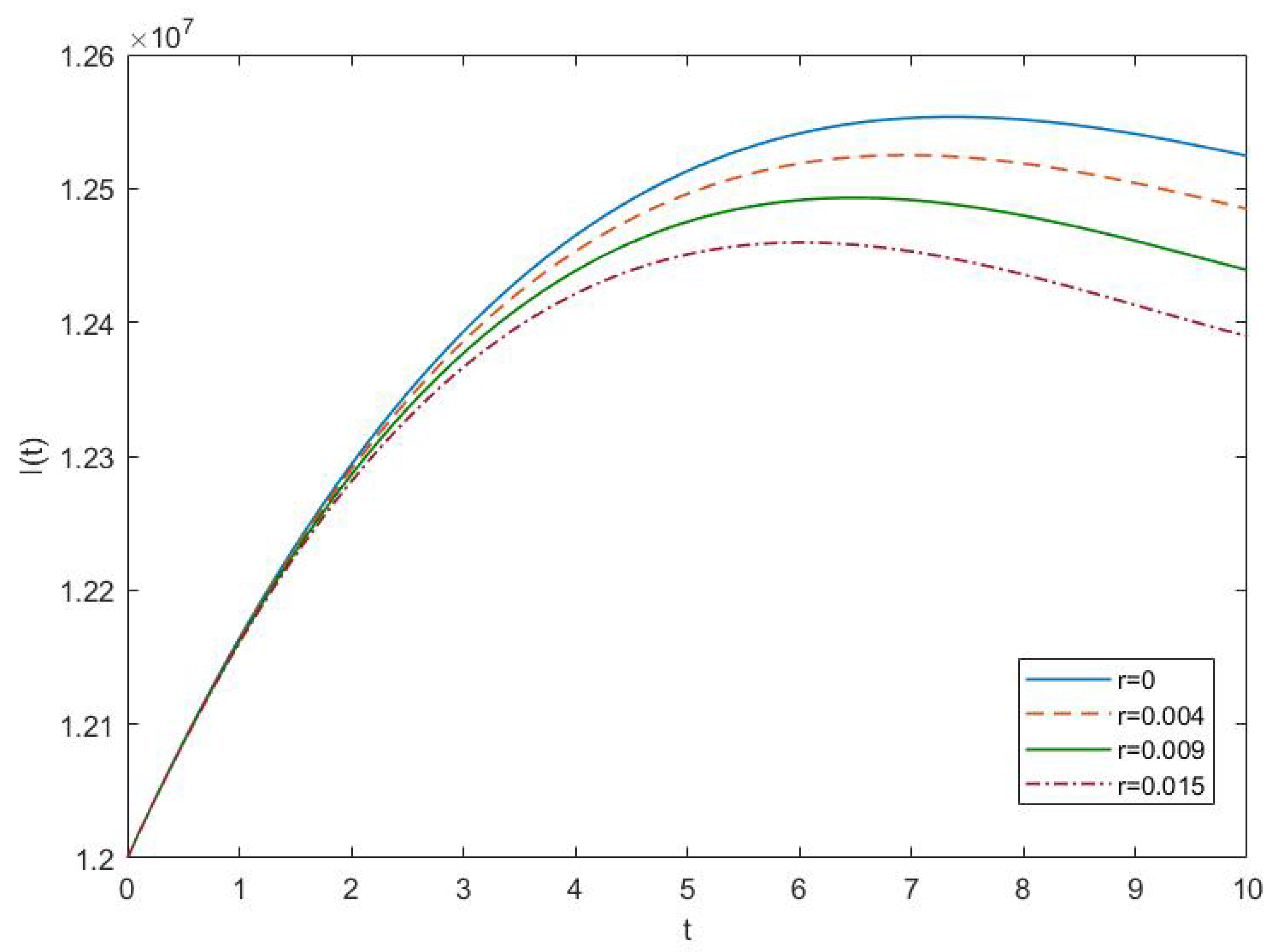
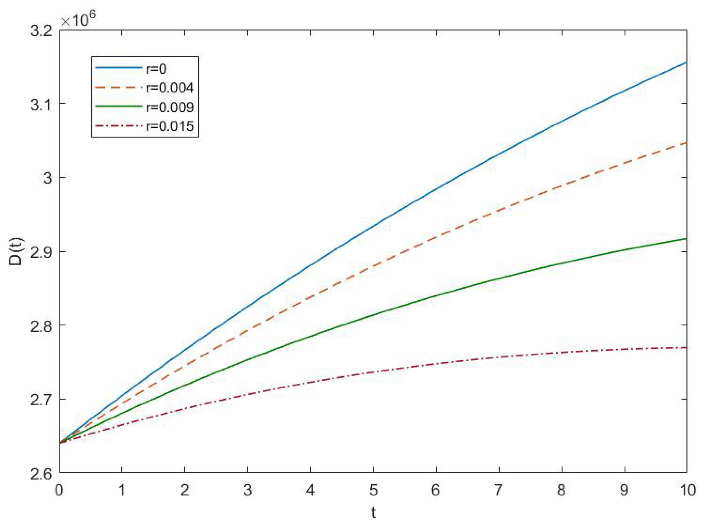
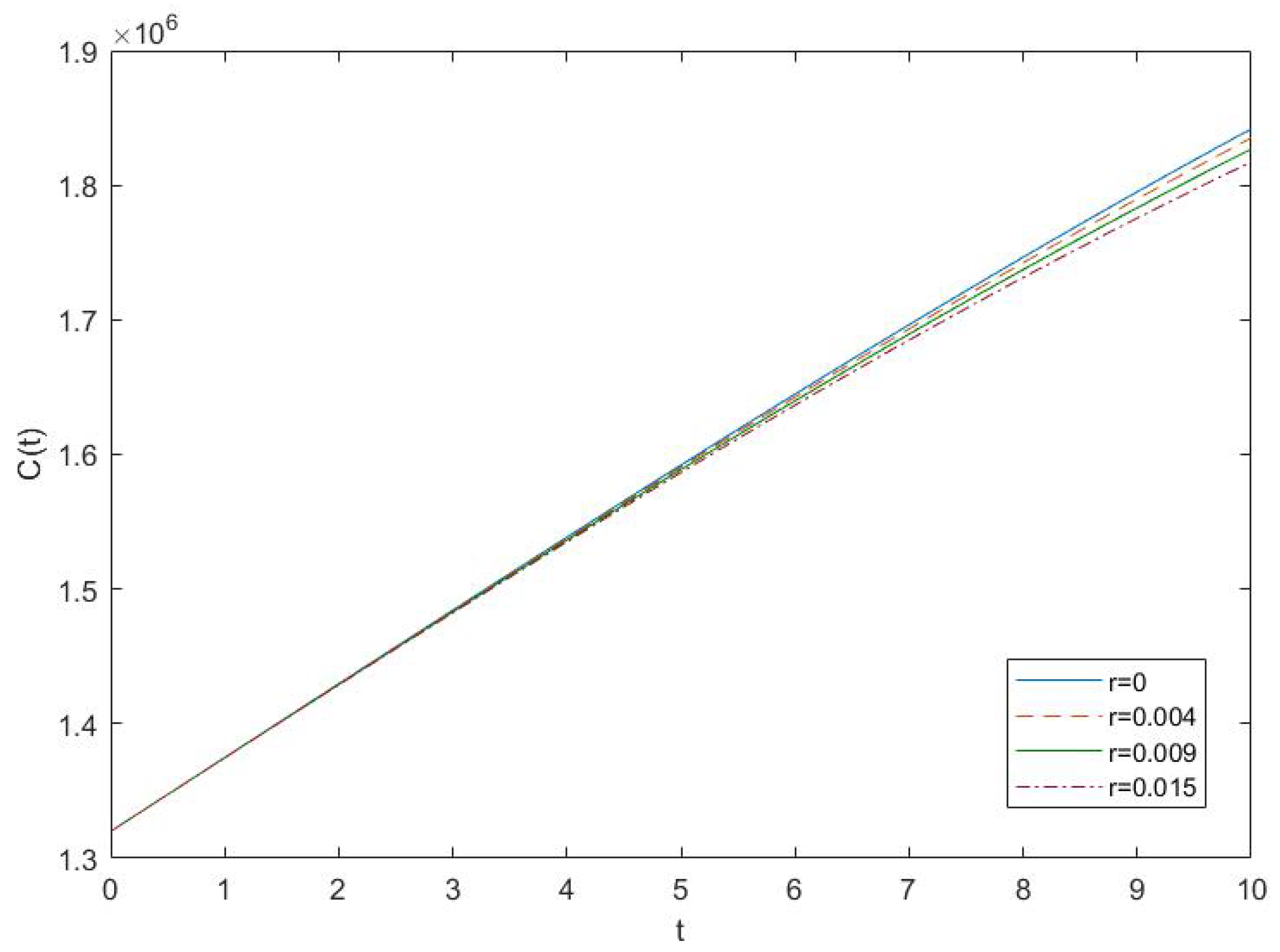
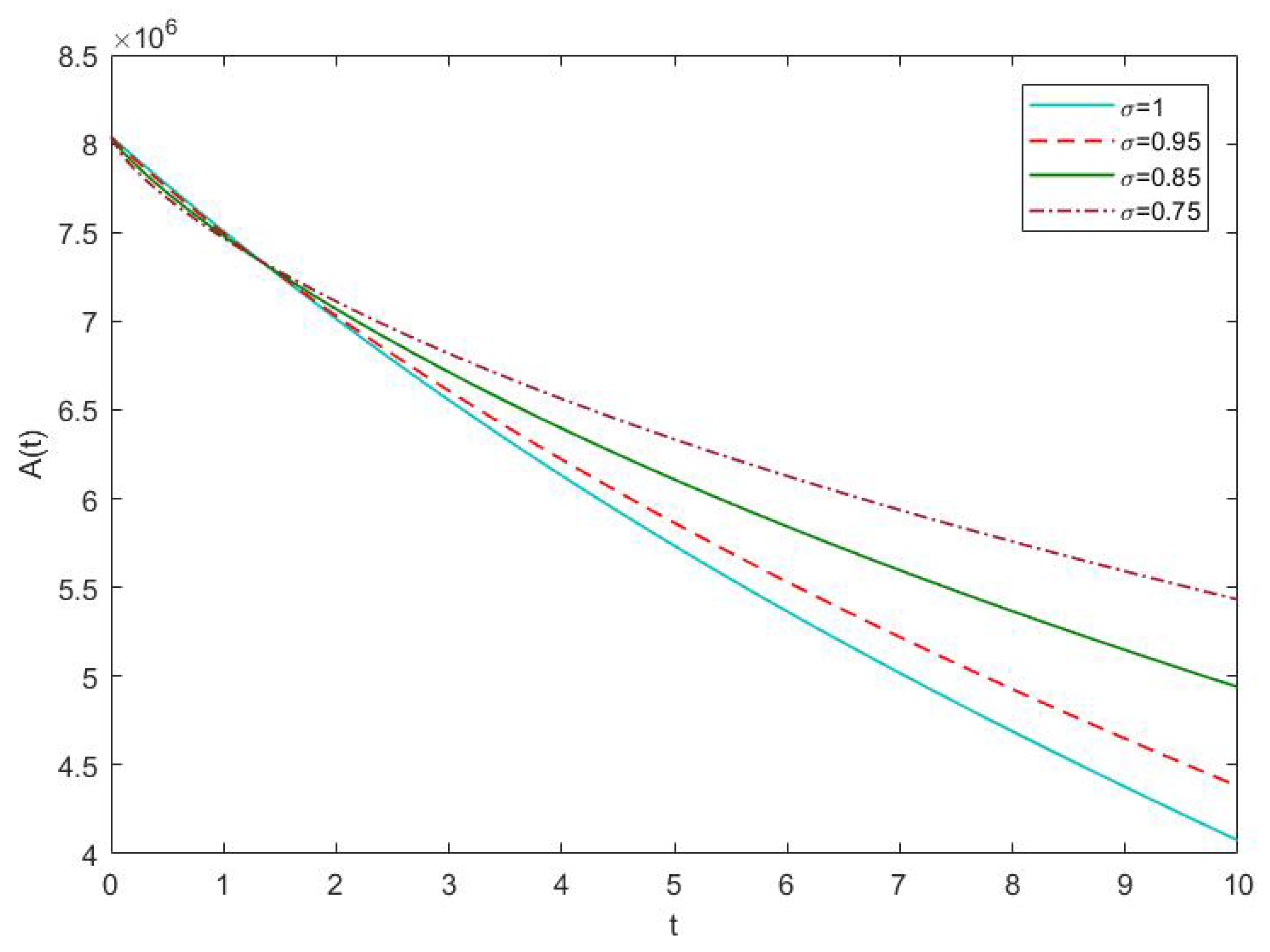
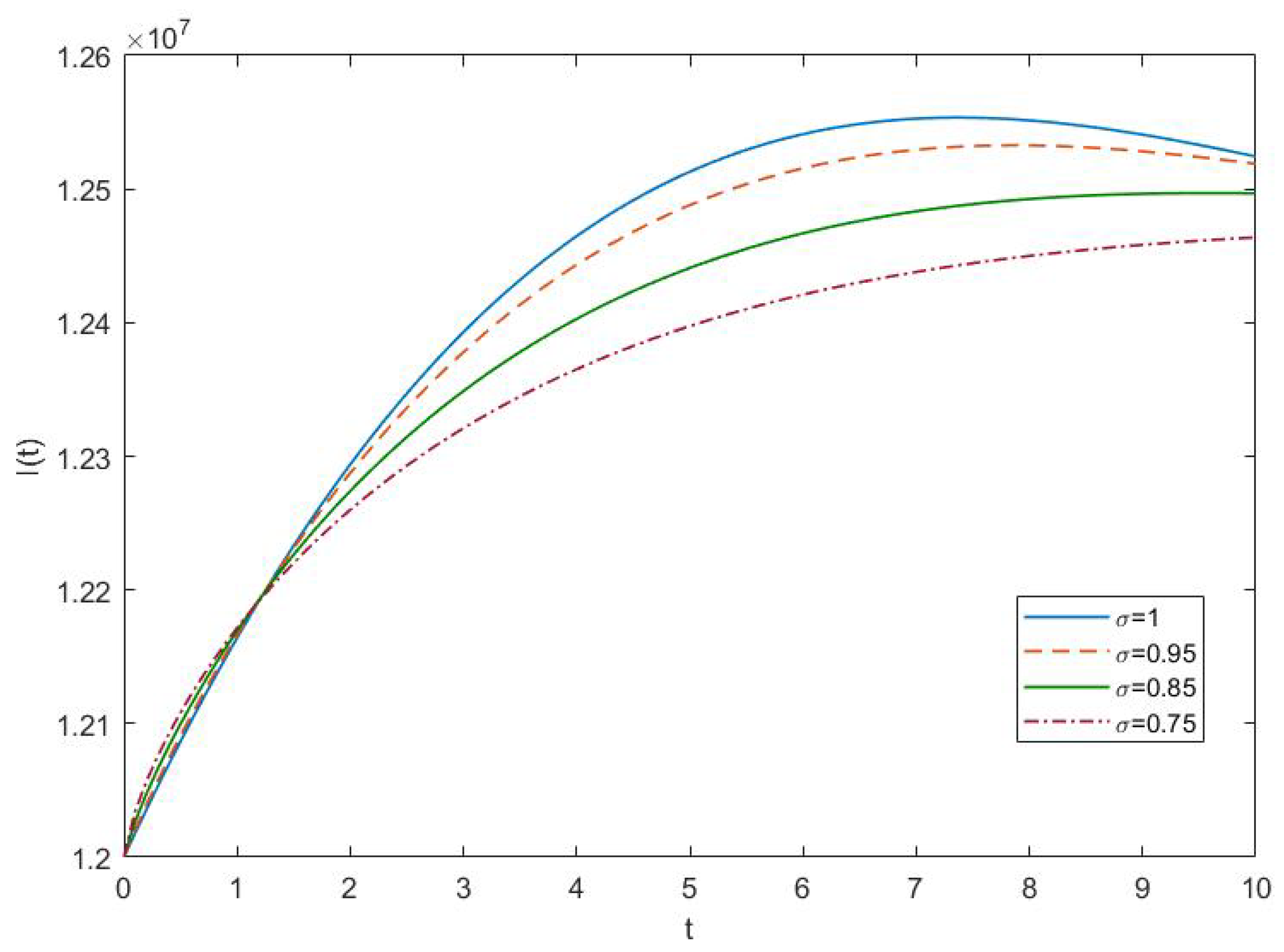
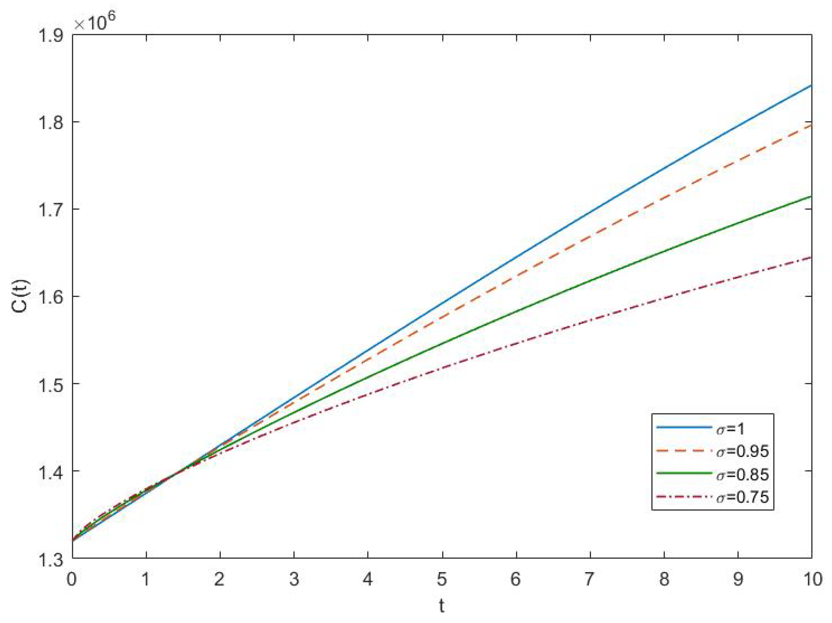
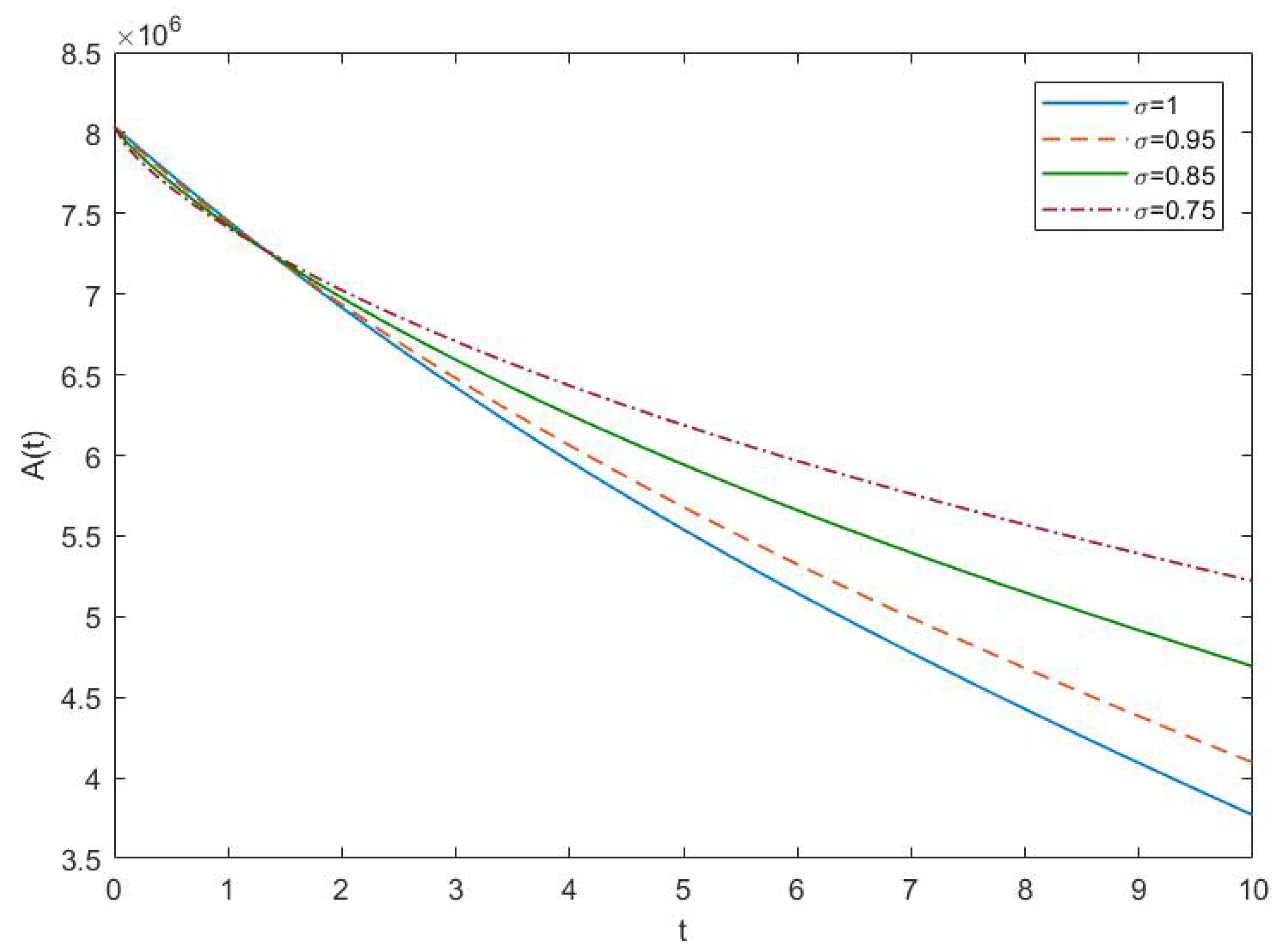
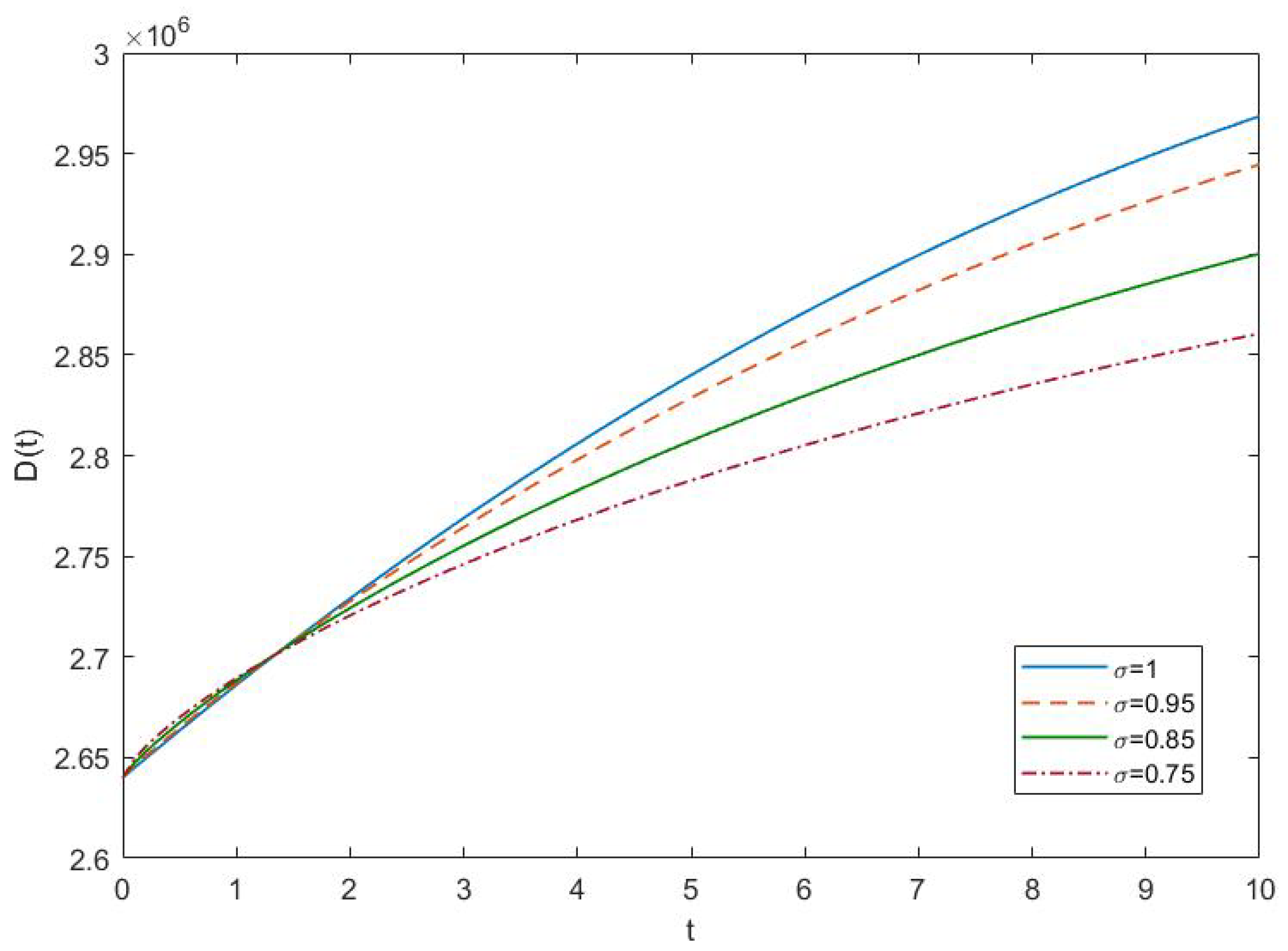
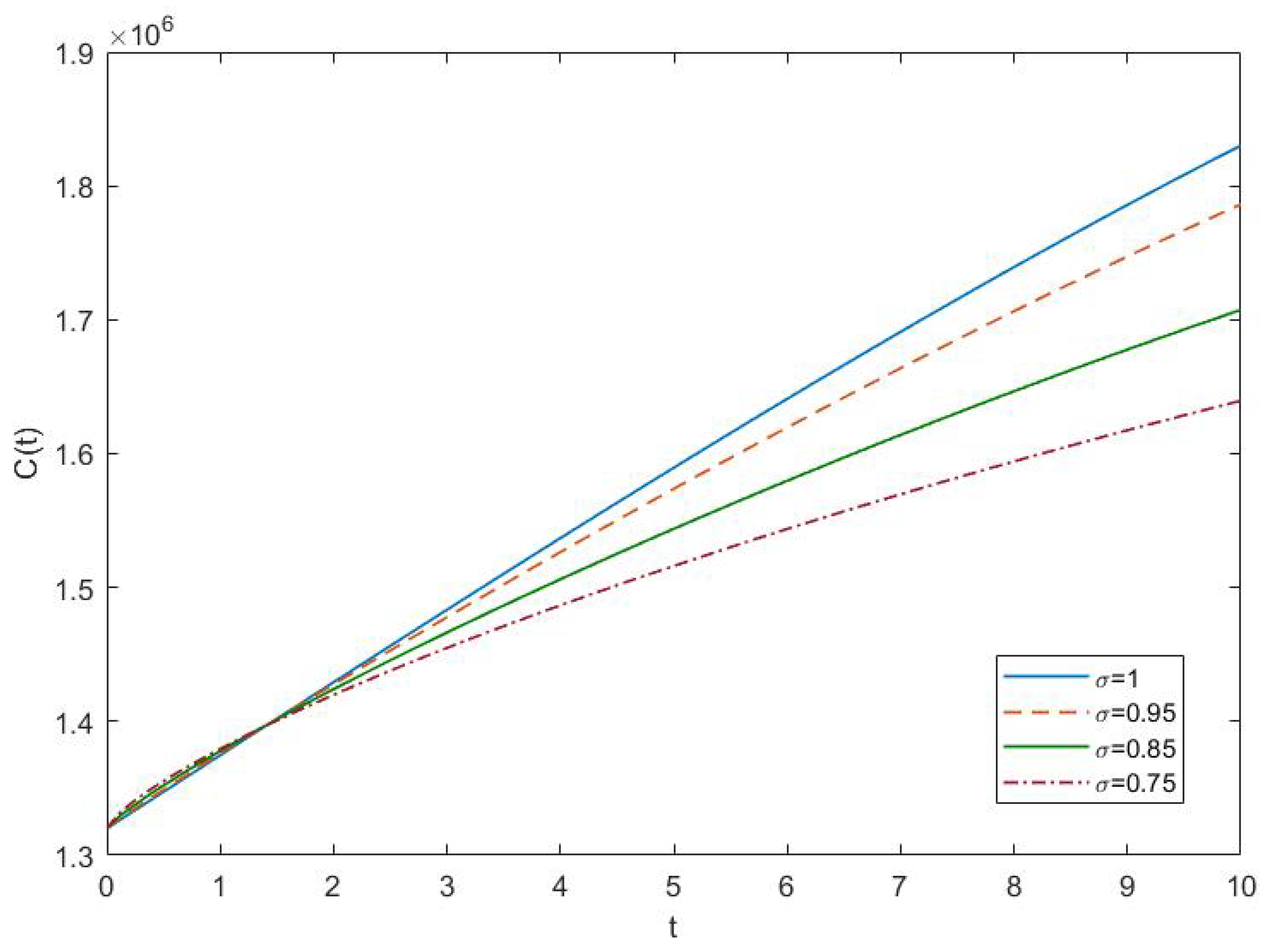
4.2. Results and Discussion

This paper’s main goal is to investigate the mathematical behavior of the fractional order dynamic model of diabetics by varying the order of the derivative and the impact of parameters $r_1$ and $r_2$ in the diabetes population model. We considered our parameter values from [16] as our model is an extension of the integer order model proposed by Mohamed Lamlili E.N. et al., and compared our results to the classical case, i.e., for $\sigma =1$. The following are the parametric values used for the simulation:

$$\begin{array}{c}\begin{array}{c}\hfill \eta =53000,{\alpha }_1=0.06,{\alpha }_2=0.007,{\alpha }_3=0.001,{\alpha }_4=0.005,{\beta }_1=0.005,\\ \hfill {\beta }_2=0.01,\mathsf{\mu }=0.012,\delta =0.012,N=24\times {10}^6,I\left(0\right)=0.5\times N,\\ \hfill D\left(0\right)=0.11\times N,C\left(0\right)=0.5\times D\left(0\right),A\left(0\right)=N-D\left(0\right)-C\left(0\right)-I\left(0\right).\end{array}\hfill \end{array}$$

We consider $r_1=r_2=r$ for the concise description of graphs. According to different values of r, Figure 1, Figure 2, Figure 3 and Figure 4 depict the behaviors of the integer-order population model from people following healthy lifestyles to people having diabetes with complications. According to Figure 1, Figure 2, Figure 3 and Figure 4, the diabetic patient’s number decreases as r rises; the same phenomenon is supported by comparable findings described in [25]. The authors concluded that diabetes patients might be sent into the remission category for longer using healthy lifestyle parameters, such as diet and exercise, leading to a significant decrease in the diabetic population.

Figure 5, Figure 6, Figure 7 and Figure 8 show the impact of the fractional order population model without the remission characteristics. It is clear from the graphs that when the order of the derivatives decreases in the fraction portion, the population to drops, and A grows. Additionally, it is evident from the graphs that the effects of fractional order derivatives begin to be felt between t = 1 and t = 2, which is relatively consistent with real-world events.

This study concludes that using fractional order derivatives reduces the population of individuals living unhealthy lives, increases the population of people living good lifestyles, and lowers the population of people with complications from diabetes. Similar types of results are found in [16].

Mohamed Lamlili E.N. et al. concluded that their classical model of the diabetic population, i.e., for $\sigma =1$, predicts a reduction in the population of individuals living unhealthy lives and an increase in the population of people living good lifestyles. Our findings for fractional order agree with those of the study by Mohamed Lamlili E.N. et al. for $\sigma =1$. Also, similar types of results can be seen in [15].

Figure 9, Figure 10, Figure 11 and Figure 12 show the impact of the fractional order population model without the remission characteristics. It is clear from the graphs that when the order of the derivatives decreases in the fraction portion, the populations corresponding to D, I, and C drop, and A grows. Additionally, it is evident from the graphs that the effects of the fractional order derivatives begin to be felt between t = 1 and t = 2, which is relatively consistent with real-world events.

This study concludes that using fractional order derivatives reduces the population of individuals living unhealthy lives, increases the population of people living good lifestyles, and lowers the population of people with complications from diabetes. Similar types of results were found in [16].

Mohamed Lamlili E.N. et al. concluded that their classical model of the diabetic population, i.e., for $\sigma =1$, indicates a reduction in the population of individuals living unhealthy lives and an increase in the population of people adopting healthier lifestyles. Our findings for the fractional order are in agreement with those of the Mohamed Lamlili E.N. et al. study for $\sigma =1$. Also, similar types of results can be seen in [15].

Figure 9, Figure 10, Figure 11 and Figure 12 show the same outcomes as Figure 5, Figure 6, Figure 7 and Figure 8, but the population of persons leading unhealthy lives decreases more quickly, and diabetic complications are quickly cured as a result of the addition of the remission parameter.

5. Conclusions

This study presented a diabetic mellitus population model with fractional order derivatives. The analysis of the proposed fractional order model with overweight/obesity was conducted. We attempted to demonstrate the influence of a healthy lifestyle on remission by incorporating two additional parameters into the framework of the diabetic population. Further, we examined the Caputo sense of the fractional order derivative on the model of the diabetic population, regardless of remission parameters. Moreover, the existence and uniqueness of the solution of the diabetes mellitus model are discussed. Non-negativity and boundedness are also examined. Subsequently, the stability analysis for the model’s equilibrium points uses the Jacobian matrix concept. Eventually, an approximation of the solutions was carried out by using the Daftardar-Gejji and Jafari method. The outcomes of the fractional order model (3) are positive and evenly bounded. Numerical simulations are then conducted to demonstrate the research findings. The graphs show the impact of the fractional order population model without the remission elements. They show that when the fractional order of derivatives decreases, the populations corresponding to D, I, and C drop, while A increases. Also, when remission parameters are considered, it can be observed that the diabetic patient’s number decreases as remission rises. Eventually, it is concluded from the displayed graphs that upon incorporating remission parameters, the population of persons leading unhealthy lives decreases more quickly and diabetic complications are quickly cured, showing a clear dependence on the remission parameters and fractional order derivative.

In the future, we will examine our fractional order diabetic population model using alternative approaches, such as treatment functions, and compare the outcomes to acquire new knowledge and insight.

References

1. World Health Organization. Global Diffusion of eHealth: Making Universal Health Coverage Achievable: Report of the Third Global Survey on eHealth; World Health Organization: Geneva, Switzerland, 2017. [Google Scholar]
2. Ogurtsova, K.; Guariguata, L.; Barengo, N.C.; Ruiz, P.L.D.; Sacre, J.W.; Karuranga, S.; Sun, H.; Boyko, E.J.; Magliano, D.J. IDF diabetes Atlas: Global estimates of undiagnosed diabetes in adults for 2021. Diabetes Res. Clin. Pr. 2022, 183, 109118. [Google Scholar] [CrossRef] [PubMed]
3. Sun, H.; Saeedi, P.; Karuranga, S.; Pinkepank, M.; Ogurtsova, K.; Duncan, B.B.; Stein, C.; Basit, A.; Chan, J.C.; Mbanya, J.C.; et al. IDF Diabetes Atlas: Global, regional and country-level diabetes prevalence estimates for 2021 and projections for 2045. Diabetes Res. Clin. Pract. 2022, 183, 109119. [Google Scholar] [CrossRef] [PubMed]
4. Roth, G. Global Burden of Disease Collaborative Network. Global Burden of Disease Study 2017 (GBD 2017) Results. Seattle, United States: Institute for Health Metrics and Evaluation (IHME), 2018. Lancet 2018, 392, 1736–1788. [Google Scholar] [CrossRef] [PubMed]
5. Korsmo-Haugen, H.K.; Brurberg, K.G.; Mann, J.; Aas, A.M. Carbohydrate quantity in the dietary management of type 2 diabetes: A systematic review and meta-analysis. Diabetes Obes. Metab. 2019, 21, 15–27. [Google Scholar] [CrossRef]
6. Boutayeb, A.; Twizell, E.; Achouayb, K.; Chetouani, A. A mathematical model for the burden of diabetes and its complications. Biomed. Eng. Online 2004, 3, 1–8. [Google Scholar] [CrossRef]
7. Sweatman, C.Z.H. Mathematical model of diabetes and lipid metabolism linked to diet, leptin sensitivity, insulin sensitivity and VLDLTG clearance predicts paths to health and type II diabetes. J. Theor. Biol. 2020, 486, 110037. [Google Scholar]
8. Al-Hussein, A.B.A.; Rahma, F.; Jafari, S. Hopf bifurcation and chaos in time-delay model of glucose-insulin regulatory system. Chaos Solitons Fractals 2020, 137, 109845. [Google Scholar] [CrossRef]
9. Kouidere, A.; Labzai, A.; Ferjouchia, H.; Balatif, O.; Rachik, M. A new mathematical modeling with optimal control strategy for the dynamics of population of diabetics and its complications with effect of behavioral factors. J. Appl. Math. 2020, 2020. [Google Scholar] [CrossRef]
10. Mollah, S.; Biswas, S. Effect of awareness program on diabetes mellitus: Deterministic and stochastic approach. J. Appl. Math. Comput. 2021, 66, 61–86. [Google Scholar] [CrossRef]
11. Mollah, S.; Biswas, S.; Khajanchi, S. Impact of awareness program on diabetes mellitus described by fractional-order model solving by homotopy analysis method. In Ricerche di Matematica; Springer: Berlin/Heidelberg, Germany, 2022; pp. 1–26. [Google Scholar]
12. Xue, D.; Zhao, C.; Chen, Y. Fractional order PID control of a DC-motor with elastic shaft: A case study. In Proceedings of the 2006 American Control Conference, Minneapolis, MN, USA, 14–16 June 2006; p. 6. [Google Scholar]
13. Gutierrez, R.E.; Rosário, J.M.; Tenreiro Machado, J. Fractional order calculus: Basic concepts and engineering applications. Math. Probl. Eng. 2010, 2010, 375858. [Google Scholar] [CrossRef]
14. Ahmed, E.; Hashish, A.; Rihan, F. On fractional order cancer model. J. Fract. Calc. Appl. Anal. 2012, 3, 1–6. [Google Scholar]
15. Srivastava, H.M.; Shanker Dubey, R.; Jain, M. A study of the fractional-order mathematical model of diabetes and its resulting complications. Math. Methods Appl. Sci. 2019, 42, 4570–4583. [Google Scholar] [CrossRef]
16. Mohamed Lamlili, E.; Boutayeb, W.; Boutayeb, A. The Dynamics of a Population of Healthy Adults, Overweight/Obese and Diabetics With and Without Complications in Morocco. In Proceedings of the International Conference on Electronic Engineering and Renewable Energy Systems, Saidia, Morocco, 20–22 May 2022; pp. 29–36. [Google Scholar]
17. Li, Y.; Chen, Y.; Podlubny, I. Stability of fractional-order nonlinear dynamic systems: Lyapunov direct method and generalized Mittag–Leffler stability. Comput. Math. Appl. 2010, 59, 1810–1821. [Google Scholar] [CrossRef]
18. Odibat, Z.M.; Shawagfeh, N.T. Generalized Taylor’s formula. Appl. Math. Comput. 2007, 186, 286–293. [Google Scholar] [CrossRef]
19. Li, H.L.; Zhang, L.; Hu, C.; Jiang, Y.L.; Teng, Z. Dynamical analysis of a fractional-order predator-prey model incorporating a prey refuge. J. Appl. Math. Comput. 2017, 54, 435–449. [Google Scholar] [CrossRef]
20. De Boor, C.; Golub, G.H. The numerically stable reconstruction of a Jacobi matrix from spectral data. Linear Algebra Appl. 1978, 21, 245–260. [Google Scholar] [CrossRef]
21. DeJesus, E.X.; Kaufman, C. Routh-Hurwitz criterion in the examination of eigenvalues of a system of nonlinear ordinary differential equations. Phys. Rev. A 1987, 35, 5288. [Google Scholar] [CrossRef]
22. Kumar, M.; Jhinga, A.; Daftardar-Gejji, V. New algorithm for solving non-linear functional equations. Int. J. Appl. Comput. Math. 2020, 6, 26. [Google Scholar] [CrossRef]
23. Daftardar-Gejji, V.; Jafari, H. An iterative method for solving nonlinear functional equations. J. Math. Anal. Appl. 2006, 316, 753–763. [Google Scholar] [CrossRef]
24. Banaś, J.; O’Regan, D. On existence and local attractivity of solutions of a quadratic Volterra integral equation of fractional order. J. Math. Anal. Appl. 2008, 345, 573–582. [Google Scholar] [CrossRef]
25. Dave, R.; Davis, R.; Davies, J. The impact of multiple lifestyle interventions on remission of type 2 diabetes mellitus within a clinical setting. Obes. Med. 2019, 13, 59–64. [Google Scholar] [CrossRef]
Figure 1. Impact of the remission parameter on the population following healthy lifestyles.
Fractalfract 07 00839 g001
Figure 2. Impact of the remission parameter on the population following unhealthy lifestyles.
Fractalfract 07 00839 g002
Figure 3. Effects of the remission parameter on diabetics without complications.
Fractalfract 07 00839 g003
Figure 4. Effects of the remission parameter on diabetics without complications.
Fractalfract 07 00839 g004
Figure 5. Impact of the fractional order on the population following healthy lifestyles, with r = 0 .
Fractalfract 07 00839 g005
Figure 6. Impact of the fractional order on the population following unhealthy lifestyles, with r = 0 .
Fractalfract 07 00839 g006
Figure 7. Effects of the fractional order on diabetics without complications with r = 0 .
Fractalfract 07 00839 g007
Figure 8. Effects of the fractional order on diabetics without complications with r = 0 .
Fractalfract 07 00839 g008
Figure 9. Impact of the fractional order and remission parameter on the population following healthy lifestyles, with r = 0.007 .
Fractalfract 07 00839 g009
Figure 10. Impact of the fractional order and remission parameter on the population following unhealthy lifestyles, with r = 0.007 .
Fractalfract 07 00839 g010
Figure 11. Effects of the remission parameter and fractional order on diabetics without complications, with r = 0.007 .
Fractalfract 07 00839 g011
Figure 12. Effects of the remission parameter and fractional order on diabetics without complications, with r = 0.007 .
Fractalfract 07 00839 g012
Disclaimer/Publisher’s Note: The statements, opinions and data contained in all publications are solely those of the individual author(s) and contributor(s) and not of MDPI and/or the editor(s). MDPI and/or the editor(s) disclaim responsibility for any injury to people or property resulting from any ideas, methods, instructions or products referred to in the content.