Abstract
The aim of this paper is to define the generalized discrete proportional derivative (GDPD) and illustrate the application of the Leibniz theorem, the binomial expansion, and Montmort’s formulas in the context of the generalized discrete proportional case. Furthermore, we introduce the generalized discrete proportional Laplace transform and determine the GDPLT of various functions using the inverse operator. The results obtained are showcased through relevant examples and validated using MATLAB.
1. Introduction
Undoubtedly, mathematics holds immense value across various disciplines, including physics, economics, and engineering [1,2,3,4,5,6,7,8]. The concept of a difference equation becomes essential when describing the evolution of a phenomenon over time. In the works of [9,10], the discrete case of the differential operator is precisely defined as
The discrete cases of derivatives (both real and complex order) and integrals can be defined using discrete fractional calculus, extending the principles of (integer-order) differential calculus [11,12,13]. Specifically, fractional derivatives in this context are synonymous with Riemann–Liouville fractional derivatives (RLFDs), and their definitions have been explored in various ways in [14,15,16,17].
Likewise, discrete fractional derivatives can be defined through various approaches. In the realm of difference calculus, particularly fractional difference calculus [10,18,19], one encounters the forward h-difference operator , which is defined as
In 1989, Miller and Ross introduced the discrete counterpart of the RLFD, elucidating numerous characteristics of the fractional difference operator [11,20]. This work not only involved proposing the discrete analogue but also encompassed the definition of various generalized difference operators. We further extended our contributions by deriving exact solutions and presenting numerical solutions for a variety of functions [21,22,23]. Notably, we introduced the discrete variant of the generalized proportional derivative, known as the generalized proportional delta operator.
In the study presented in [24], the authors investigated lower regularized incomplete gamma functions, showcasing their utility in demonstrating the existence and uniqueness of solutions for fractional differential equations involving nonlocal fractional derivatives. Exploring a new frontier, [25] delves into the realm of solutions for a distinct category of nonlinear generalized proportional fractional differential inclusions. This exploration encompasses scenarios where the right-hand side incorporates a Caratheodory-type multivalued nonlinearity, extending the analysis to infinite intervals. Furthermore, [26] introduces a comprehensive two-step design approach aimed at implementing a fractional-order proportional integral controller tailored for a specific class of fractional-order plant models. Motivated by the preceding discussions and incentives, the principal objective of this paper is to delve into the concept of the GDPD. This investigation involves demonstrating the practical applicability of Leibniz’s theorem, binomial expansion, and Montmort’s formulas within the generalized discrete proportional setting.
Expanding on prior research, we have extended the discrete form of the generalized proportional differential operator. Its inverse has been skillfully employed to derive fundamental formulas, enabling the computation of closed-form solutions and numerical solutions for distinct categories of finite and infinite series within the domain of number theory. Remarkably, the application of this operator to advance the theoretical foundations of the discrete version remains unparalleled in the existing literature.
A clear distinction often arises between numerical solutions and closed-form solutions in prevalent methodologies. Discrepancies emerge, necessitating the individual determination of the error factor. Remarkably, when utilizing the generalized proportional difference operator and its inverse, the need for a separate determination of the error factor is obviated. The equivalence between numerical solutions and closed form solutions is consistently observed in our methodologies.
In this article, the generalized proportional delta operator has been proposed. Section 2 studies the generalized discrete proportional case of the Leibnitz theorem, binomial expansion, and Montmort’s formulas by defining the generalized proportional difference operator. In Section 3, we establish the inverse generalized proportional delta operator and derives exact and numerical solutions of various functions. In Section 4, we discuss the applications in various types of arithmetic progression (AP) of finite series involving the operator . In Section 5, we define the generalized proportional discrete Laplace transform (GDPLT) and obtain the GDPLT of various functions. To demonstrate our findings, appropriate examples are supplied and confirmed using MATLAB in Section 6. Finally, the conclusion of this paper is given in Section 7.
2. Basic Definitions and Results
Prior to presenting and proving our results, we lay the foundation by introducing essential definitions and lemmas. This section unveils fundamental concepts and provides preliminary results that will prove crucial in our subsequent discussions.
Definition 1
([27]). A Conformable Differential Operator is defined by
which represents the α-derivative of . Here, is conformable provided the function is differentiable at t and .
Definition 2
([23]). Let be real- or complex-valued function on . Then, the forward -difference operator on is defined by
Remark 1
([19,23]). When and , the difference operator becomes the generalized difference operator , defined as .
Definition 3.
By Definition 1, the generalized proportional delta operator for the function is defined by
Lemma 1.
If is the usual lead operator, then
Proof.
From the usual lead operator , we write
When , (5) becomes . Then, from (3) and (5), we obtain
By comparing Equations (6) and (7), we complete the proof. □
Lemma 2.
If a, b are constants and , are any real- or complex-valued functions on , then
- (i)
- ;
- (ii)
- ;
- (iii)
- ;
- (iv)
- .
Proof.
The proof follows by Definition 3. □
Definition 4.
By Definition 3, the second order of is defined as and, in general, the order of is defined as .
The following are easy deductions.
- (i)
- For the positive integers p, q and , ;
- (ii)
- For and ;
- (iii)
- (iv)
- For the function ,and hence,
- (v)
- (vi)
- (vii)
The following theorem presents the generalized discrete proportional case of Leibniz’s theorem.
Theorem 1.
Let and , , be any two functions. Then,
Proof.
Define the operators , , , and hence as
From (4) and (10), we have = where
From the above expression, we obtain
The results follow from the binomial theorem, (9)–(11). □
Next, we establish the generalized discrete proportional form of the binomial expansion.
Theorem 2.
For the generalized discrete proportional case of the binomial expansion is given by
Proof.
From (4), we have Furthermore, . This implies
The proof follows by taking on (13) and using binomial theorem. □
We now introduce the discrete case of Montmort’s generalized proportional formula.
Lemma 3.
If the series converges, then
Proof.
Using the lead operator we can get
Now, the proof follows by using the binomial expansion. □
3. Inverse of the Generalized Proportional Difference Operator
In this section, we establish the inverse of the generalized proportional difference operator and present explicit formulas for partial sums involving higher powers of the geometric arithmetic progression. Additionally, we illustrate the application of these formulas through relevant examples, providing a comprehensive understanding of their utility in practical scenarios.
Definition 5.
By Definition 3, we define the inverse of the generalized proportional difference operator represented as follows. If , then
where is constant and the order inverse generalized proportional difference operator represented by is defined as
Lemma 4.
Let , w(t)=1, and . Then,
Proof.
From (3) and (15), we get the proof. □
Lemma 5.
If , ℓ is positive real and , then
Proof.
The proof is followed by (15) and the relation
□
The operator methods of summation on are as follows.
Theorem 3.
Assume that , is any function of t and . Then, we obtain,
where
Proof.
For a function , we find
hence, we obtain
From (19) and (15), we find
and hence by (20), we obtain
where . Equations (17) and (21), along with the binomial theorem, are now used to support the proof. □
4. Applications in Various Sorts of A.P. Finite Series Involving
Utilizing as a tool, we derive expressions for the sums of both arithmetico-geometric progressions and arithmetico-double geometric progressions in the realm of number theory.
The following theorem presents the general formula for the summation of higher powers in an arithmetico-geometric progression.
Theorem 4.
Let , , and . Then,
where .
Proof.
Theorem 5.
Let , , and . Then,
where .
Proof.
The following theorem provides the formula for the sum of an arithmetico-double geometric progression.
Theorem 6.
If and , then
where
Proof.
which yields from (15) that
which yields from (15) that
which yields from (15) that
Now, we proceed with the same process for , and this completes the proof. □
Remark 2.

The following Table 1 is a comparison of Theorem 3, Theorem 4, Theorem 5 and Theorem 6.

Table 1.
Comparison.
Remark 3.
Researchers can analyze discrete generalized proportional differences and inverse differences across various functions. Readers may apply this operator in Newton’s law of cooling to reduce errors.
5. Applications of the Generalized Discrete Proportional Laplace Transform Using
Within this section, we delve into the application of to determine the GDPLT. The subsequent definition elucidates the GDPLT.
Definition 6.
By Definition 3, let be a function of t defined for and let . Then, the generalized discrete proportional Laplace transform is defined by
where and and denote the inverse of the generalized discrete proportional Laplace transform.
Lemma 6
(Numerical solution). Let be a function of t defined for and . Then,
Proof.
The proof follows from the relation
as and (3). □
Lemma 7
(Exact solution). Let be a function of and . Then, the generalized discrete proportional Laplace transform of is given by
Proof.
The generalized discrete proportional Laplace transform of is
Hence,
The proof is complete. □
The following Proposition 1 establishes the equivalence between the numerical solution and the exact solution of the generalized discrete proportional Laplace transform.
Proposition 1.
Let be a function of and . Then, the numerical and exact solutions of the generalized discrete proportional Laplace transform of are equal, which is given by
Lemma 8.
Let and . Then,
Proof.
The proof follows by (3) and (15). □
Lemma 9.
Let and . Then,
Proof.
Using (3), (15) and Lemma 8, the proof is complete. □
Proposition 2.
Let be a unit step function of t and . Then, the generalized discrete proportional Laplace transform of is given by
Proof.
Taking in (37), we get
Using (43) and (44) in (46), we get the proof. □
Lemma 10.
Let and . Then,
Proof.
The proof follows by (3) and (15). □
Lemma 11.
Let and . Then,
Proof.
Using (3), (15) and Lemma 8, the proof is complete. □
Proposition 3.
Let be a function of t and . Then, the generalized discrete proportional Laplace transform of is given by
Proof.
Taking in (37), we get
Using (47) and (48) in (50), we get the proof. □
Lemma 12.
Let and . Then,
Proof.
The proof follows by (3) and (15). □
Lemma 13.
Let and . Then,
Proof.
Using (3), (15) and Lemma 8, the proof is complete. □
Theorem 7.
Let be a function of t and . Then, the generalized discrete proportional Laplace transform of is given by
Proof.
Taking in (37), we get
Using (51) and (52) in (54), we get the proof. □
Lemma 14.
Let and . Then,
Proof.
The proof follows by (3) and (15). □
Lemma 15.
Let and . Then,
Proof.
Using (3), (15) and Lemma 8, the proof is complete. □
Theorem 8.
Let be a function of t and . Then, the generalized discrete proportional Laplace transform of is given by
or
and
where and .
Proof.
Taking in (37), we get
Using (55) and (56) in (60), we get (57), and equating the coefficients of real and imaginary parts, we get (58) and (59). □
Lemma 16.
Let and . Then,
Proof.
Using (3), (15) and Lemma 8, the proof is complete. □
Proposition 4.
Let be a function of t and . Then, the generalized discrete proportional Laplace transform of is given by
Proof.
Taking in (37), we get
Using (43) and (61) in (63), we get the proof. □
6. Numerical Examples
Within this section, we showcase examples and figures that demonstrate the application of the GDPD and the generalized discrete proportional Laplace transform to various functions.
Definition 3 is demonstrated using the following example.
Example 1.
Let and . The generalized proportional difference of a function as follows:
- (i)
- at , , we have the following:
- (ii)
- and at , , we have the following:
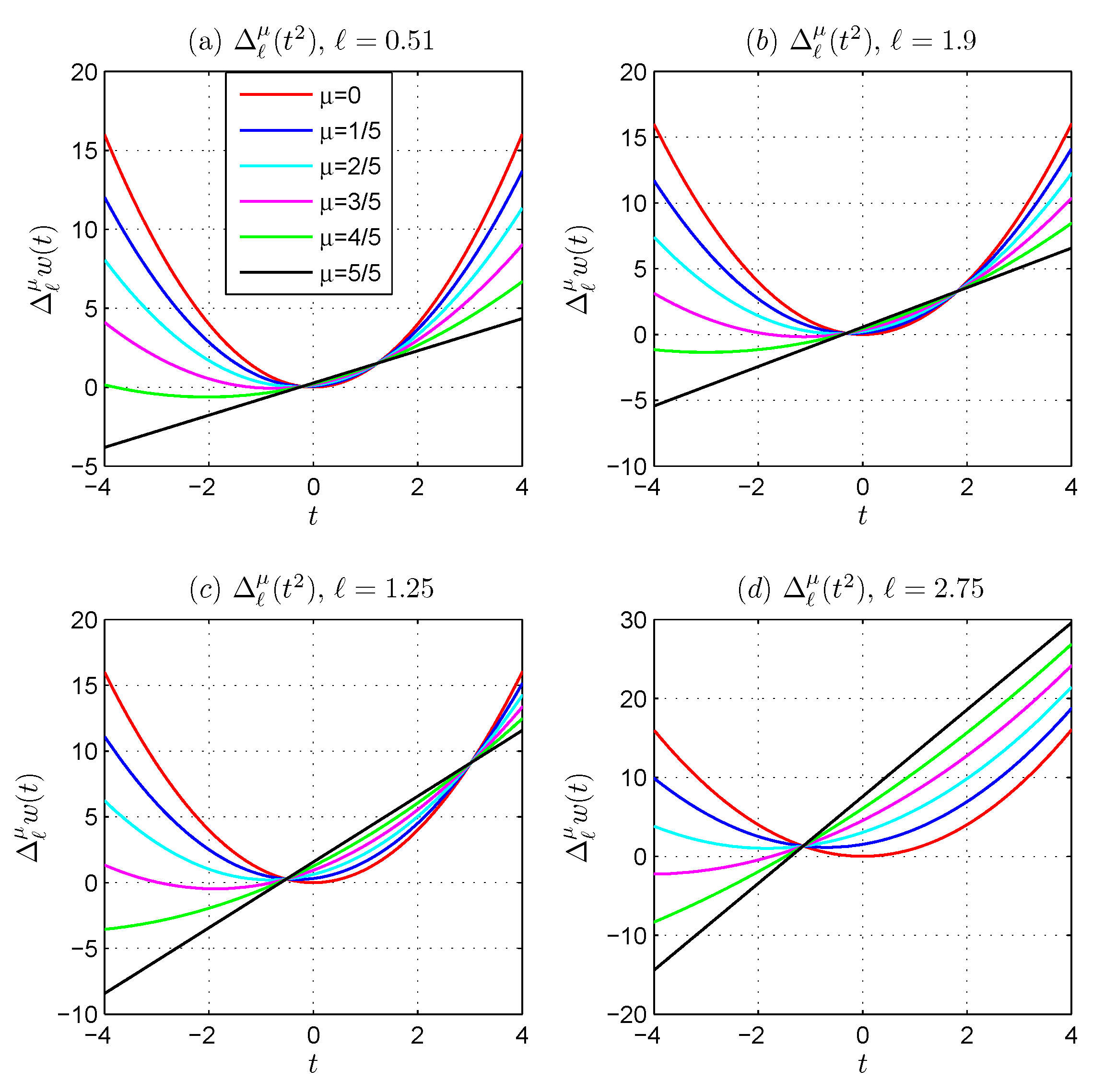
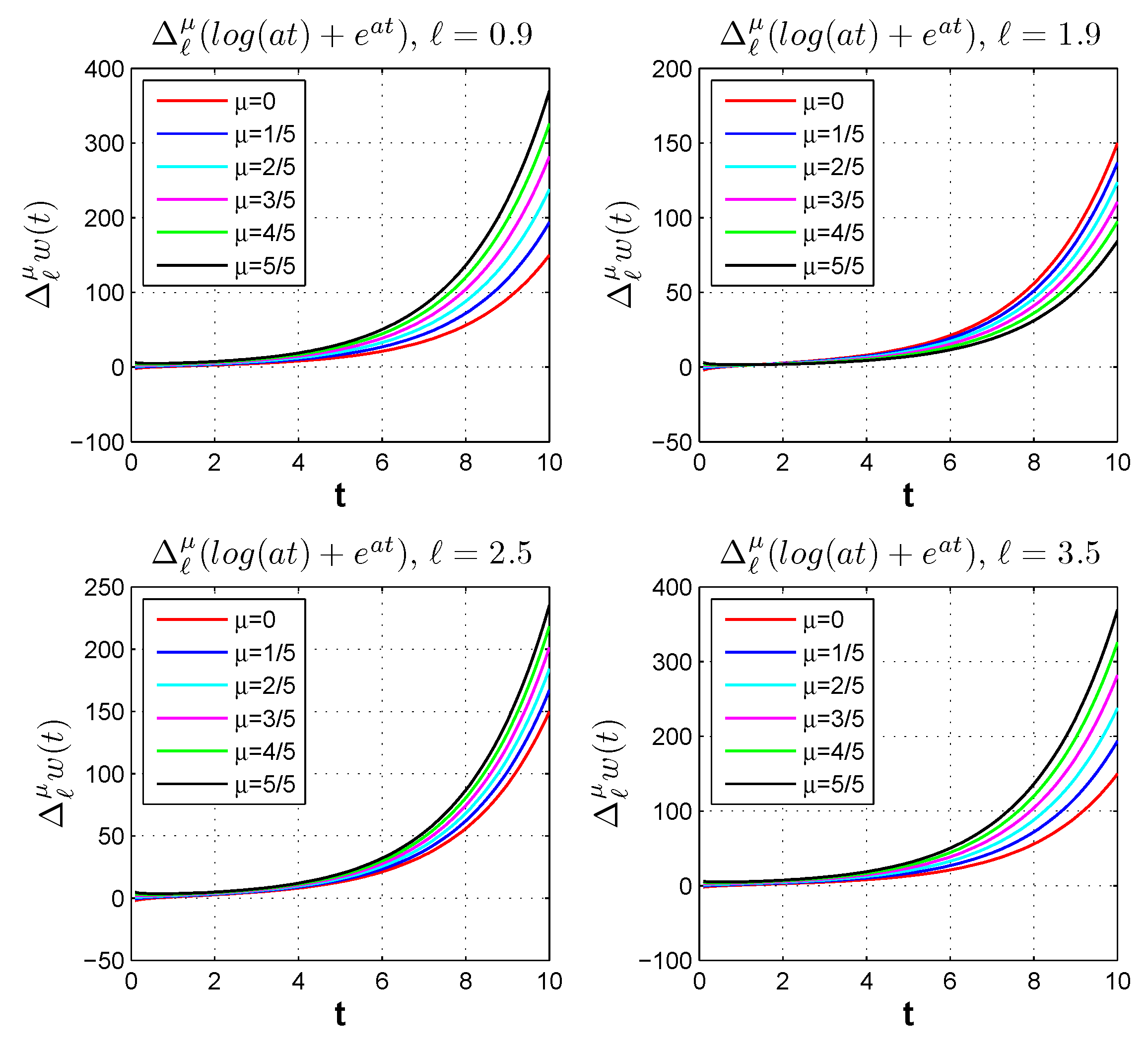
The following Figure 1a–d shows the graphical representation for the given fuction
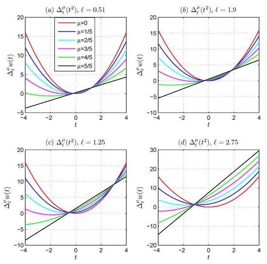
Figure 1.
Generalized proportional difference of for different shift values ℓ.
In Figure 1, we visually depict the transformation of the generalized proportional differences of from to as increases from 0 to 1. Moreover, the graphical representation in Figure 2 depicts the generalized proportional difference of for various shift values ℓ.
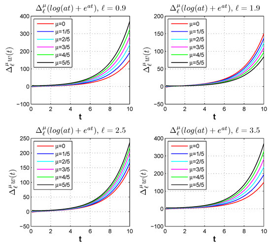
Figure 2.
Generalized proportional difference of for different shift values ℓ.
The efficacy of Theorem 2 is demonstrated through the illustrative example presented in Example 2.
Example 2.
If θ is expressed in degrees with positive real values in an anticlockwise orientation, then
.
The effectiveness of Theorem 4 is verified through the following illustrative Example 3.
Example 3.
By taking and in (16), we obtain
The effectiveness of Theorem 4 is verified through the following illustrative example.
Example 4.
Using , , and in (22), we obtain
where and .
The effectiveness of Theorem 5 is verified through the following illustrative Example 5.
Example 5.
Using , , and in (5), we get
where and .
The effectiveness of Theorem 6 is verified through the following illustrative Example 6.
Example 6.
Substituting , , , and in Theorem 6, we get
where and .
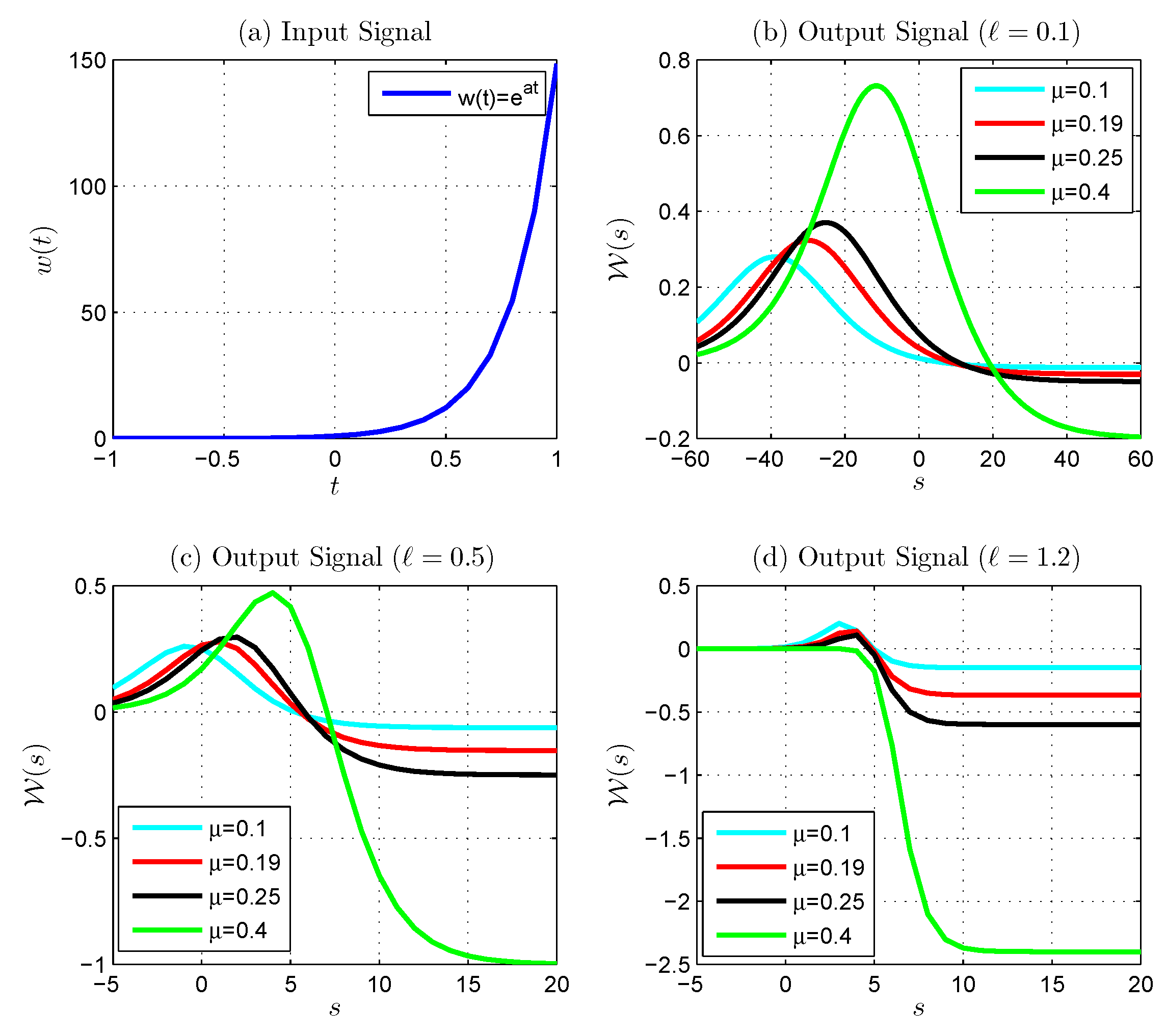
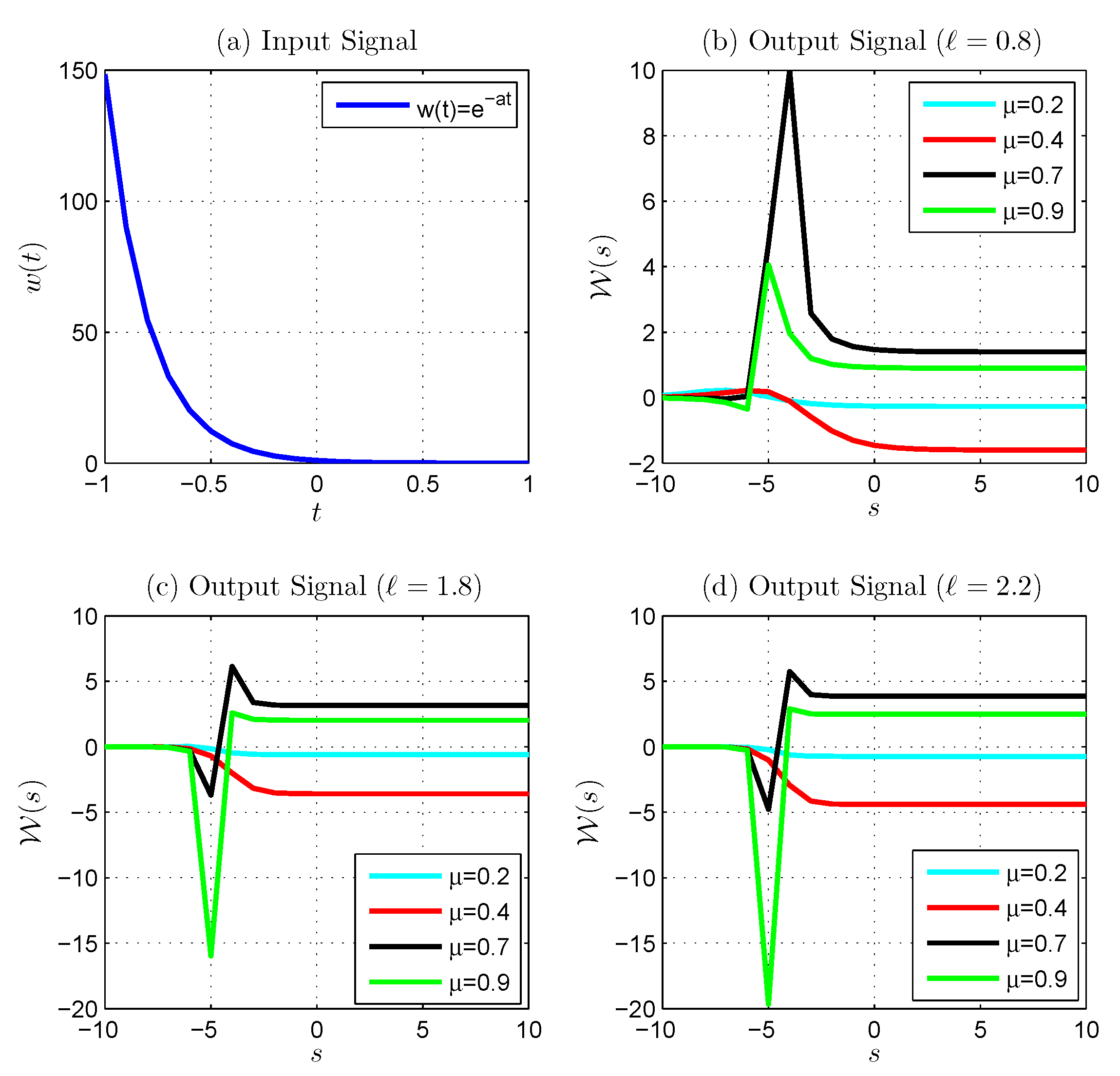
The following Figure 3, Figure 4, Figure 5, Figure 6 and Figure 7 show the generalized discrete proportional Laplace transform of a unit step function, the generalized discrete proportional Laplace transform of the generalized discrete proportional Laplace transform of the generalized discrete proportional Laplace transform of and the generalized discrete proportional Laplace transform of .
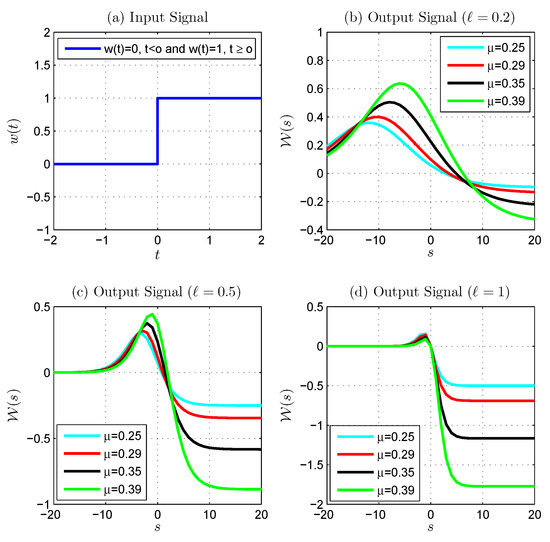
Figure 3.
Generalized discrete proportional Laplace transform of the unit step function: (a) is the input signal, (b–d) show the output signal with fixed ℓ () and various .
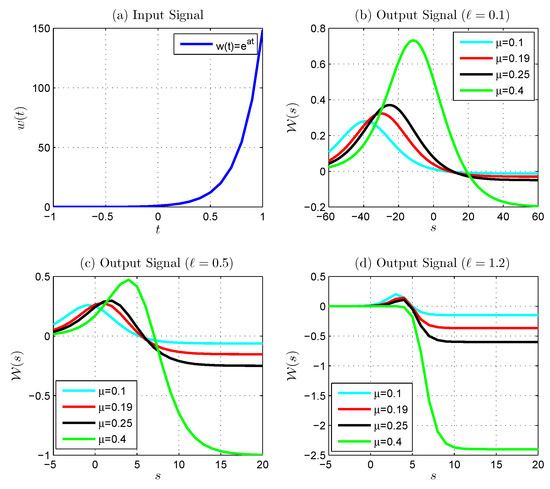
Figure 4.
Generalized discrete proportional Laplace transform of : (a) is the input signal, (b–d) shows the output signal with fixed ℓ () and various .
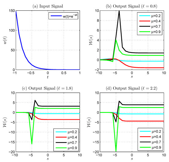
Figure 5.
Generalized discrete proportional Laplace transform of : (a) is the input signal, (b–d) shows the output signal with fixed ℓ () and various .
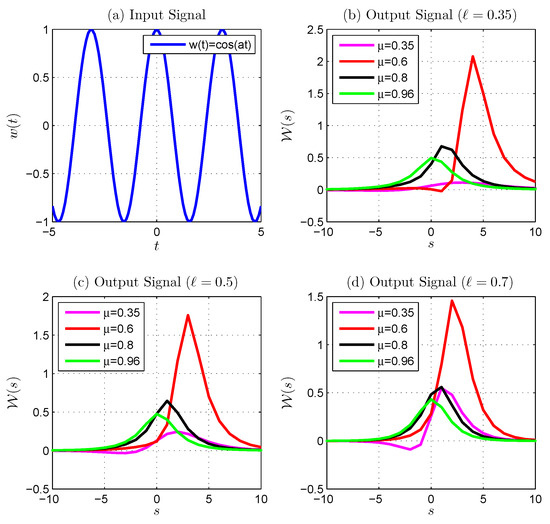
Figure 6.
Generalized discrete proportional Laplace transform of : (a) is the input signal, (b–d) shows the output signal with fixed ℓ () and various .
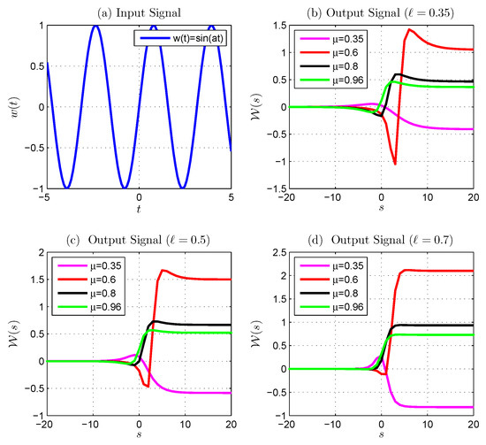
Figure 7.
Generalized discrete proportional Laplace transform of : (a) is the input signal, (b–d) shows the output signal with fixed ℓ () and various .
7. Conclusions
This article explores the generalized discrete proportional case of Leibnitz’s theorem, binomial expansion, and Montmort’s equations by establishing the difference operator. The authors developed the inverse generalized proportional delta operator and obtained exact and numerical solutions for diverse functions. We also addressed applications in various types of APs of finite series involving the operator, and defined and obtained the GDPLT of various functions. We provide and confirm MATLAB examples to demonstrate our findings. Similarly, one can find the generalized discrete proportional Laplace transform of other functions. Readers (researchers) can discover several applications in the fields of control systems and engineering, as well as image processing. Our future studies will continue in this vein.
Author Contributions
R.P. and M.R., writing—original draft: R.P. methodology: R.P., M.R. and H.G., conceptualization: R.P. and S.S., supervision: R.P., M.R. and S.S., investigation: R.P., M.R., H.G. and S.S. All authors have read and agreed to the published version of the manuscript.
Funding
This research was funded by “Researchers Supporting Project number (RSPD2023R683), King Saud University, Riyadh, Saudi Arabia”. This work was also funded by the Centre for Nonlinear Systems, Chennai Institute of Technology (CIT), India, funding number CIT/CNS/2023/RP-005.
Data Availability Statement
There is no data contained in this article.
Conflicts of Interest
The authors declare no conflict of interest.
References
- Moumen, A.; Mennouni, A.; Bouye, M. A novel Vieta–Fibonacci projection method for solving a system of fractional integro differential equations. Mathematics 2023, 11, 3985. [Google Scholar] [CrossRef]
- Malinowska, A.B.; Torres, D.F.M. Generalized natural boundary conditions for fractional variational problems in terms of the Caputo derivative. Comput. Math. Appl. 2010, 59, 3110–3116. [Google Scholar] [CrossRef]
- Michal, F.; JinRong, W.; Michal, P. Fractional integral equations. Fractional Order Equations and Inclusions; De Gruyter: Berlin, Germany; Boston, MA, USA, 2017; pp. 37–90. [Google Scholar]
- Jafari, H.; Tuan, N.A.; Ganji, R.M. A new numerical scheme for solving pantograph type nonlinear fractional integro-differential equations. J. King Saud Univ. 2021, 33, 101185. [Google Scholar] [CrossRef]
- Sabatier, J.; Agrawal, O.P.; Machado, J.A.T. Advances in Fractional Calculus; Springer: Dordrecht, The Netherlands, 2007. [Google Scholar]
- Almeida, R.; Torres, D.F.M. Necessary and sufficient conditions for the fractional calculus of variations with Caputo derivatives. Commun. Nonlinear Sci. Numer. Simul. 2011, 16, 1490–1500. [Google Scholar] [CrossRef]
- Magin, R.L. Fractional Calculus in Bio Engineering; Begell House: Danbury, CT, USA, 2006. [Google Scholar]
- Micula, S. An iterative numerical method for fractional integral equations of the second kind. J. Comput. Appl. Math. 2018, 339, 124–133. [Google Scholar] [CrossRef]
- Mickens, R.E. Difference Equations; Van Nostrand Reinhold Company: New York, NY, USA, 1990. [Google Scholar]
- Agarwal, R.P. Difference Equations and Inequalities; Marcel Dekker: New York, NY, USA, 2000. [Google Scholar]
- Miller, K.S.; Ross, B. An Introduction to the Fractional Calculus and Fractional Differential Equations; Wiley: New York, NY, USA, 1993. [Google Scholar]
- Samko, S.G.; Kilbas, A.A.; Marichev, O.I. Fractional Integrals and Derivatives, Translated from the 1987 Russian Original; Gordon and Breach: Yverdon, Switzerland, 1993. [Google Scholar]
- Kang, Y.; Xie, Y.; Lu, J.; Jiang, J. On the nonexistence of non-constant exact periodic solutions in a class of the Caputo fractional-order dynamical systems. Nonlinear Dyn. 2015, 82, 1259–1267. [Google Scholar] [CrossRef]
- Almeida, R.; Torres, D.F.M. Calculus of variations with fractional derivatives and fractional integrals. Appl. Math. Letter. 2009, 22, 1816–1820. [Google Scholar] [CrossRef]
- Frederico, G.S.F.; Torres, D.F.M. Fractional conservation laws in optimal control theory. Nonlinear Dyn. 2008, 53, 215–222. [Google Scholar] [CrossRef]
- El-Nabulsi, R.A.; Torres, D.F.M. Necessary optimality conditions for fractional action-like integrals of variational calculus with Riemann–Liouville derivatives of order (α, β). Math. Methods Appl. Sci. 2007, 30, 1931–1939. [Google Scholar] [CrossRef]
- Mozyrska, D.; Torres, D.F.M. Minimal modified energy control for fractional linear control systems with the Caputo derivative. Carpathian J. Math. 2010, 26, 210–221. [Google Scholar]
- Bastos, N.R.O.; Ferreira, R.A.C.; Torres, D.F.M. Discrete time fractional variational problems. Signal Process 2011, 91, 513–524. [Google Scholar] [CrossRef]
- Ferreira, R.A.C.; Torres, D.F.M. Fractional h-difference equations arising from the calculus of variations. Appl. Anal. Discret. Math. 2011, 5, 110–121. [Google Scholar] [CrossRef]
- Miller, K.S.; Ross, B. Fractional Difference Calculus, in Univalent Functions, Fractional Calculus, and Their Applications; Horwood: Chichester, UK, 1989; pp. 139–152. [Google Scholar]
- Xavier, G.B.A.; Rajiniganth, P. Finite series and closed form solution of nth order α difference equation. Int. J. Pure Appl. Math. 2016, 90, 671–681. [Google Scholar]
- Xavier, G.B.A.; Rajiniganth, P.; Chandrasekar, V. Finite series and closed form solution of second order α-difference equation. Int. J. Pure Appl. Math. 2014, 90, 177–188. [Google Scholar] [CrossRef][Green Version]
- Xavier, G.B.A.; Rajiniganth, P.; Chandrasekar, V.; Manuel, M.M.S. Forward (α, β)-difference operator and its some applications in number theory. Int. J. Appl. Math. 2012, 25, 109–124. [Google Scholar]
- Abdeljawad, Z.L.T.; Jarad, F. On existence–uniqueness results for proportional fractional differential equations and incomplete gamma functions. Adv. Differ. Equ. 2020, 2020, 641. [Google Scholar]
- Abbas, M.I.; Hristova, S. Existence nesults of Non linear generalized proportional fractional differential inclusions via the diagonalization technique. AIMS Math. 2021, 76, 12832–12844. [Google Scholar] [CrossRef]
- Swarnaka, J. Discrete time realization of fractional order proportional integral controller for a class of fractional order system. Numer. Algebr. Control. Optim. 2022, 12, 309–320. [Google Scholar] [CrossRef]
- Laura, A.L.G.; Grace, K.B. The calculus of proportional α-derivatives. Rose-Hulman Undergrad. Math. J. 2017, 18, 20–42. [Google Scholar]
Disclaimer/Publisher’s Note: The statements, opinions and data contained in all publications are solely those of the individual author(s) and contributor(s) and not of MDPI and/or the editor(s). MDPI and/or the editor(s) disclaim responsibility for any injury to people or property resulting from any ideas, methods, instructions or products referred to in the content. |
© 2023 by the authors. Licensee MDPI, Basel, Switzerland. This article is an open access article distributed under the terms and conditions of the Creative Commons Attribution (CC BY) license (https://creativecommons.org/licenses/by/4.0/).

