Non-Markovian Persistent Random Walk Model for Intracellular Transport

Abstract

Transport of vesicles and organelles inside cells consists of constant-speed bidirectional movement along cytoskeletal filaments interspersed by periods of idling. This transport shows many features of anomalous diffusion. In this paper, we develop a non-Markovian persistent random walk model for intracellular transport that incorporates the removal rate of organelles. The model consists of two active states with different speeds and one resting state. The organelle transitions between states with switching rates that depend on the residence time the organelle spends in each state. The mesoscopic master equations that describe the average densities of intracellular transport in each of the three states are the main results of the paper. We also derive ordinary differential equations for the dynamics for the first and second moments of the organelles’ position along the cell. Furthermore, we analyse models with power-law distributed random times, which reveal the prevalence of the Mittag-Leffler resting state and its contribution to subdiffusive and superdiffusive behaviour. Finally, we demonstrate a non-Markovian non-additivity effect when the switching rates and transport characteristics depend on the rate of organelles removal. The analytical calculations are in good agreement with numerical Monte Carlo simulations. Our results shed light on the dynamics of intracellular transport and emphasise the effects of rest times on the persistence of random walks in complex biological systems.

1. Introduction

Transport processes within eukaryotic cells bear striking similarities to the intricate networks found in large cities. Cytoskeletal networks, analogous to roads and highways, crisscross cells, and facilitate the transport of various cargoes. Intracellular transport is a fundamental biological process involving the movement of molecules, proteins, and organelles from one location to another within cells. It relies on a combination of passive diffusion and ATP-driven movement along cytoskeletal filaments. This process is crucial to maintaining cellular structure, function, and survival, and is involved in essential cellular activities such as growth, division, and signaling. Dysregulation of intracellular transport has been implicated in numerous diseases, including cancer. Therefore, understanding the mechanisms and regulation of intracellular transport is of great importance for both basic cell biology research and clinical applications. In neurons, long-range intracellular transport is even more critical, as its malfunctioning has been linked to adult-onset neurodegenerative diseases, including Alzheimer’s, Parkinson’s, and Huntington’s disease [1].

Vesicles and organelles have been observed to undergo bidirectional motion along cytoskeletal filaments, periodically pausing for finite time intervals. These cargoes utilise molecular motors of opposite polarity in rapid succession [2,3], facilitating their transportation over long distances [4]. The two major families of motors involved in this process are kinesins and dyneins [5,6]. Kinesins transport vesicles along microtubules toward the plus ends, facilitating material transport from the cell interior toward the cortex (anterograde movement). Dyneins move material toward the microtubule minus ends, moving from the cell periphery to the cell interior (retrograde movement). Cytoplasmic dynein predominantly facilitates the minus-end directed long-range transport along microtubules (MTs) [7], and its activity is regulated by multifunctional adaptors such as dynactin [8].

Various modeling approaches have been reviewed to understand intracellular transport [2,9,10], including Markovian models such as reaction–diffusion models [11,12], Brownian ratchet models [13], random walk models [14,15], intermittent search processes [16,17], and exclusion models [18,19,20]. While most of these approaches treat microtubules implicitly, some models explicitly consider them, allowing the investigation of the influence of cytoskeleton topology on intracellular transport [21,22]. A Markovian model of particle diffusion with spatially varying diffusivity shows non-ergodic behaviour [23] frequently observed experimentally in intracellular transport, which was also modelled using non-Markovian fractional Brownian motion [24]. Several multi-state Markovian models exhibit anomalous diffusive regimes before transitioning into normal diffusion at longer times [22,25,26], or even subdiffusion due to topological trapping at longer times [21] or due to non-Markovian run-length-dependent detachment rate of cargo from a microtubule [27]. The effect of advection on diffusive particles was studied using the mobile–immobile model where the particle switch between mobile and immobile states with finite rates [28] and with power-law and mixed trapping time distributions [29]. The non-Markovian mobile-immobile model without advection was used to model the diffusion of excitons in layered perovskites and transition metal dichalcogenides [30].

Given the complexity of intracellular space, cytoskeleton topology, and various interactions within cells, it is not surprising that intracellular transport deviates from standard Brownian diffusion and displays anomalous diffusion [31,32,33,34,35,36,37]. In cellular and molecular biology, anomalous diffusion is also highly heterogeneous [38]. Experimental studies have observed different non-Brownian regimes of diffusion at various time scales [24,27,39,40,41,42,43,44,45,46,47,48,49,50,51,52]. The intracellular environment is highly crowded with macromolecules, subcellular compartments, and confinement domains, leading to subdiffusion at small time scales (less than tens of milliseconds) [53,54,55,56] which transitions to superdiffusion associated with the activity of molecular motors. Whether this superdiffusion persists at longer time scales or if it represents an intermediate regime before transitioning into further normal or subdiffusion regimes is still a subject of debate. Also, the long-time subdiffusion could originate from different mechanisms. At longer times, the influence of cytoskeleton topology [21] and the heterogeneity of the transport process come into play, leading to spurious subdiffusion [24]. In spite of this, the anomalous nature of intracellular transport suggests that non-Markovian models could be viable.

The non-Markovian nature of intracellular transport has been modelled using random walks [27], fractional Brownian motion [24,51,52] and Levy walks [57] and combinations of FBM and CTRW [46] and CTRW and Levy walk [49]. The later stochastic model consists of altering phases of active motion with constant velocity interchanged with periods of passive dynamics. Depending on the distribution of times in the two phases of motion, the model shows transitions from normal diffusive to superdiffusive and to ballistic behavior [58,59,60,61]. Recently, Han et al. [62] (see also [63]) proposed a three-state self-reinforcing random walk model involving Mittag–Leffler distributed rest:

$$\frac{\partial p_{\pm }}{\partial t}\pm \nu \frac{\partial p_{\pm }}{\partial x}=-\lambda p_{\pm }(x,t)+r_{\pm }{\tau }_0^{-\beta }{\mathcal{D}}_t^{1-\beta }{p}_0(x,t),$$

(1)

$$\frac{\partial p_0}{\partial t}=\lambda p_{+}(x,t)+\lambda p_{-}(x,t)-(r_{+}+r_{-}){\tau }_0^{-\beta }{\mathcal{D}}_t^{1-\beta }{p}_0(x,t).$$

(2)

Here, $p_{+}$ and $p_{-}$ are PDFs of particles moving in the positive and negative direction. The running times are exponentially distributed with the rate $\lambda$. The PDF $p_0(x,t)$ describes the rest states drawn from the Mittag-Leffler distribution with parameter $\beta$ and ${\mathcal{D}}_t^{1-\beta }$ denotes the Riemann–Liouville fractional derivative given by:

$${\mathcal{D}}_t^{1-\beta }{p}_0(x,t)={\displaystyle \frac{1}{\mathsf{\Gamma }\left(\beta \right)}}\frac{\partial }{\partial t}{\int }_0^t{\displaystyle \frac{p_0(x,t^{\prime })}{{(t-t^{\prime })}^{1-\beta }}}d{t}^{\prime },(0<\beta <1).$$

(3)

Three densities satisfy the following normalisation condition:

$${\int }_{-\infty }^{+\infty }(p_{+}(x,t)+p_{-}(x,t)+p_0(x,t))dx=1.$$

(4)

Parameters $r_{+}$ and $r_{-}$ describe the probabilities of transitions from the rest. In the self-reinforcing random walk model [62], these probabilities depend on time and space. This three-state self-reinforcing random walk model is characterised by superdiffusive behaviour at intermediate times and by subdiffusion at a longer time scale.

Clearly, in reality, the speeds of cargoes in anterograde and retrograde directions are not equal, since they are powered by different motors. Therefore, in this paper, we analyse intracellular transport using a one-dimensional three-state persistent random walk model with different speeds of cargoes in anterograde and retrograde directions $v_{+}$ and $v_{-}$ that generalises the system (1)–(3). We suggest a model in which cargo transitions between moving states and resting states with zero velocity are non-Markovian. We consider the case when the rate of transitions depends on the running time. In order to take into account the random duration of cargo trajectories observed in experiments [24,52], we introduce a removal rate that terminates trajectories at random times. This effect was not considered in a recent paper [64]. The constant removal rate corresponds to the exponentially distributed duration of trajectories. The structure of the paper is as follows. In Section 2, we set up the Three-State Model with a residence time variable and derive the equations for the structured densities in two active states and one passive state. In Section 3, the mesoscopic master equations for densities in all three states are introduced. Specific examples of the Markovian Three-State Model and the Three-State Model with Mittag-Leffler distributed resting times are considered, and equations are derived for the first and second moments. The analytical results of Section 3 are compared in Section 4, in which we perform Monte Carlo simulations. Finally, we discuss our results in Section 5 and give a summary and conclusions in Section 6.

2. Three-State Transport Model with a Residence Time Variable

We consider a model in which cargo randomly switches between three possible states: Two states in which the cargoes move with a constant speed ${\nu }_{+}>0$ (state A) or ${\nu }_{-}>0$ (state R) and a resting state (state 0) in which the cargoes do not move. In this section, we aim to develop a stochastic intracellular transport model to describe the non-Markovian dynamics of intracellular transport.

We introduce the densities that are functions of running and residence time $\tau$ [65,66,67,68]. Consider $n_A(x,t,\tau )$ and $n_R(x,t,\tau )$ the densities of cargoes at point x at time t whose residence time in an active state (state A or state R, respectively) lies in the interval $(\tau ,\tau +d\tau )$. The density of cargoes in a resting state is $n_0(x,t,\tau )$. The balance equations for structured densities can be written as [66]:

$$\frac{\partial n_A}{\partial t}+\frac{\partial n_A}{\partial \tau }+{\nu }_{+}\frac{\partial n_A}{\partial x}=-{\lambda }_A\left(\tau \right)n_A-{\theta }_A{n}_A,$$

(5)

$$\frac{\partial n_R}{\partial t}+\frac{\partial n_R}{\partial \tau }-{\nu }_{-}\frac{\partial n_R}{\partial x}=-{\lambda }_R\left(\tau \right)n_R-{\theta }_R{n}_R,$$

(6)

$$\frac{\partial n_0}{\partial t}+\frac{\partial n_0}{\partial \tau }=-{\lambda }_0\left(\tau \right)n_0-{\theta }_0{n}_0,$$

(7)

where ${\lambda }_A\left(\tau \right)$, ${\lambda }_R\left(\tau \right)$ and ${\lambda }_0\left(\tau \right)$ are the switching rates that depend on $\tau$ and ${\theta }_A$, ${\theta }_R$ and ${\theta }_0$ are the constant removal rates. We assume that the residence time of all cargoes at $t=0$ equals zero. In this case, the initial conditions are:

$$n_j(x,0,\tau )=p_j^0\left(x\right)\delta \left(\tau \right),j=A,R,0,$$

(8)

where $p_j^0\left(x\right)$ represents the initial densities $(0\le \tau \le t)$.

Three escape (switching) rates, ${\lambda }_A\left(\tau \right)$, ${\lambda }_R\left(\tau \right)$, ${\lambda }_0\left(\tau \right)$ appearing in (5)–(7) can be defined as [69]:

$${\lambda }_j\left(\tau \right)={\displaystyle \frac{{\psi }_j\left(\tau \right)}{{\mathsf{\Psi }}_j\left(\tau \right)}},j=A,R,0,$$

(9)

where ${\psi }_j\left(\tau \right)$ are PDFs of the residence times in corresponding states and ${\mathsf{\Psi }}_j\left(\tau \right)={\int }_{\tau }^{\infty }{\psi }_j\left(u\right)du$ are the survival functions. Our approach is very flexible and can be used for various forms of the residence time probability distribution. This flexibility is important, since recently, the non-exponential PDF of the residence time was found in experiments [27].

The boundary conditions at zero running time ($\tau =0$) can be written as follows:

$$\begin{gathered} n_A(x,t,0)={\alpha }_A{\int }_0^t{\lambda }_A\left(\tau \right)n_A(x,t,\tau )d\tau +{\beta }_A{\int }_0^t{\lambda }_R\left(\tau \right)n_R(x,t,\tau )d\tau + \\ {\gamma }_A{\int }_0^t{\lambda }_0\left(\tau \right)n_0(x,t,\tau )d\tau , \end{gathered}$$

(10)

$$\begin{gathered} n_R(x,t,0)={\alpha }_R{\int }_0^t{\lambda }_A\left(\tau \right)n_A(x,t,\tau )d\tau +{\beta }_R{\int }_0^t{\lambda }_R\left(\tau \right)n_R(x,t,\tau )d\tau + \\ {\gamma }_R{\int }_0^t{\lambda }_0\left(\tau \right)n_0(x,t,\tau )d\tau , \end{gathered}$$

(11)

$$\begin{gathered} n_0(x,t,0)={\alpha }_0{\int }_0^t{\lambda }_A\left(\tau \right)n_A(x,t,\tau )d\tau +{\beta }_0{\int }_0^t{\lambda }_R\left(\tau \right)n_R(x,t,\tau )d\tau + \\ {\gamma }_0{\int }_0^t{\lambda }_0\left(\tau \right)n_0(x,t,\tau )d\tau . \end{gathered}$$

(12)

These equations describe the switching process to the states A, R, and resting state 0. If the cargo moves in the positive direction, it can switch with rate ${\lambda }_A\left(\tau \right)$ to the opposite direction with the probability ${\alpha }_R$, to the resting state with the probability ${\alpha }_0$, or continue in the same direction with the probability ${\alpha }_A$. The cargo moving in the negative direction can switch with rate ${\lambda }_B\left(\tau \right)$ to the opposite direction with the probability ${\beta }_A$, to the resting state with the probability ${\beta }_0$, or continue in the same direction with the probability ${\beta }_R$. Finally, for the resting cargo, it can switch with rate ${\lambda }_0\left(\tau \right)$ to cargo moving in the positive direction with the probability ${\gamma }_A$, to cargo moving in the negative direction with the probability ${\gamma }_R$, or remain at rest again with the probability ${\gamma }_0$. Obviously,

$${\alpha }_A+{\alpha }_R+{\alpha }_0=1,{\beta }_A+{\beta }_R+{\beta }_0=1,{\gamma }_A+{\gamma }_R+{\gamma }_0=1.$$

(13)

The product ${\lambda }_j\left(\tau \right)n_j(x,t,\tau )$ gives the escape rate corresponding to a particular residence time $\tau$. If we denote the escape rates from the states A, R and 0 by $i_A(x,t)$, $i_R(x,t)$ and $i_0(x,t)$, correspondingly. They can be obtained by integrating ${\lambda }_j{n}_j$ over variable $\tau$ from 0 to t [67]:

$$i_j(x,t)={\int }_0^t{\lambda }_j\left(\tau \right)n_j(x,t,\tau )d\tau ,j=A,R,0.$$

(14)

It follows from Equations (10)–(12) and (14) that

$$n_A(x,t,0)={\alpha }_A{i}_A(x,t)+{\beta }_A{i}_R(x,t)+{\gamma }_A{i}_0(x,t),$$

(15)

$$n_R(x,t,0)={\alpha }_R{i}_A(x,t)+{\beta }_R{i}_R(x,t)+{\gamma }_R{i}_0(x,t),$$

(16)

$$n_0(x,t,0)={\alpha }_0{i}_A(x,t)+{\beta }_0{i}_R(x,t)+{\gamma }_0{i}_0(x,t).$$

(17)

We solve Equations (5)–(7) using the method of characteristics: For active states $(0\le \tau <t)$:

$$n_A(x,t,\tau )=n_A(x-{\nu }_{+}\tau ,t-\tau ,0)e^{-{\int }_0^{\tau }{\lambda }_A\left(u\right)du}{e}^{-{\theta }_A\tau }.$$

(18)

$$n_R(x,t,\tau )=n_R(x+{\nu }_{-}\tau ,t-\tau ,0)e^{-{\int }_0^{\tau }{\lambda }_R\left(u\right)du}{e}^{-{\theta }_R\tau }.$$

(19)

For resting state $(0\le \tau <t)$

$$n_0(x,t,\tau )=n_0(x,t-\tau ,0)e^{-{\int }_0^{\tau }{\lambda }_0\left(u\right)du}{e}^{-{\theta }_0\tau }.$$

(20)

One can see that all solutions (18)–(20) contain an exponential factor $e^{-{\int }_0^{\tau }{\lambda }_j\left(s\right)ds}$, which is recognised as the survival function ${\mathsf{\Psi }}_j\left(\tau \right)$:

$${\mathsf{\Psi }}_j\left(\tau \right)=e^{-{\int }_0^{\tau }{\lambda }_j\left(u\right)},j=A,R,0.$$

(21)

Using Equations (10)–(12), the solutions in (18) can be rewritten using the survival function from (21) and the escape rates (switching terms) as follows:

$$\begin{gathered} n_A(x,t,\tau )=\left[{\alpha }_A{i}_A(x-{\nu }_{-}\tau ,t-\tau )+{\beta }_A{i}_R(x-{\nu }_{-}\tau ,t-\tau )+{\gamma }_A{i}_0(x-{\nu }_{-}\tau ,t-\tau )\right]\times \\ {\mathsf{\Psi }}_A\left(\tau \right)e^{-{\theta }_A\tau }, \end{gathered}$$

(22)

$$\begin{gathered} n_R(x,t,\tau )=\left[{\alpha }_R{i}_A(x+{\nu }_{-}\tau ,t-\tau )+{\beta }_R{i}_R(x+{\nu }_{-}\tau ,t-\tau )+{\gamma }_R{i}_0(x+{\nu }_{-}\tau ,t-\tau )\right]\times \\ {\mathsf{\Psi }}_R\left(\tau \right)e^{-{\theta }_R\tau }, \end{gathered}$$

(23)

$$n_0(x,t,\tau )=\left[{\alpha }_0{i}_A(x,t-\tau )+{\beta }_0{i}_R(x,t-\tau )+{\gamma }_0{i}_0(x,t-\tau )\right]{\mathsf{\Psi }}_0\left(\tau \right)e^{-{\theta }_0\tau }.$$

(24)

Notice that the residence time PDF, ${\psi }_j\left(\tau \right)$, is related to the switching rate, ${\lambda }_j\left(\tau \right)$, as follows [69]:

$${\psi }_j\left(\tau \right)={\lambda }_j\left(\tau \right)e^{-{\int }_0^{\tau }{\lambda }_j\left(u\right)du},j=A,R,0.$$

(25)

3. Mesoscopic Master Equations

Now, we introduce the mesoscopic densities for all three states: $p_A(x,t)$, $p_R(x,t)$ and $p_0(x,t)$. The functions $p_A$ and $p_R$ are the densities for cargoes moving in a positive/negative direction and $p_0$ is the density of cargoes with a resting state. These densities can be obtained by integrating the structured densities $n_j(x,t,\tau )$ over residence time variable $\tau$:

$$p_j(x,t)={\int }_0^t{n}_j(x,t,\tau )d\tau ,j=A,R,0.$$

(26)

By differentiating (26) with respect to time t and using (5)–(7), we obtain the mesoscopic master equations for $p_A$, $p_R$ and $p_0$:

$$\begin{gathered} \frac{\partial p_A}{\partial t}=n_A(x,t,t)-{\int }_0^t{\lambda }_A\left(\tau \right)n_A(x,t,\tau )d\tau -{\nu }_{+}{\int }_0^t\frac{\partial n_A}{\partial x}d\tau -{\int }_0^t\frac{\partial n_A}{\partial \tau }d\tau \\ -{\theta }_A{\int }_0^t{n}_A(x,t,\tau )d\tau , \end{gathered}$$

(27)

$$\begin{gathered} \frac{\partial p_R}{\partial t}=n_R(x,t,t)-{\int }_0^t{\lambda }_R\left(\tau \right)n_R(x,t,\tau )d\tau +{\nu }_{-}{\int }_0^t\frac{\partial n_R}{\partial x}d\tau -{\int }_0^t\frac{\partial n_R}{\partial \tau }d\tau \\ -{\theta }_R{\int }_0^t{n}_R(x,t,\tau )d\tau , \end{gathered}$$

(28)

$$\frac{\partial p_0}{\partial t}=n_0(x,t,t)-{\int }_0^t{\lambda }_0\left(\tau \right)n_0(x,t,\tau )d\tau -{\int }_0^t\frac{\partial n_0}{\partial \tau }d\tau -{\theta }_0{\int }_0^t{n}_0(x,t,\tau )d\tau .$$

(29)

Using (10)–(29), we rewrite the system of equations using the escape rates $i_A$, $i_R$, and $i_0$:

$$\frac{\partial p_A}{\partial t}+{\nu }_{+}\frac{\partial p_A}{\partial x}=-(1-{\alpha }_A)i_A(x,t)+{\beta }_A{i}_R(x,t)+{\gamma }_A{i}_0(x,t)-{\theta }_A{p}_A,$$

(30)

$$\frac{\partial p_R}{\partial t}-{\nu }_{-}\frac{\partial p_R}{\partial x}={\alpha }_R{i}_A(x,t)-(1-{\beta }_R)i_R(x,t)+{\gamma }_R{i}_0(x,t)-{\theta }_R{p}_R,$$

(31)

$$\frac{\partial p_0}{\partial t}={\alpha }_0{i}_A(x,t)+{\beta }_0{i}_R(x,t)-(1-{\gamma }_0)i_0(x,t)-{\theta }_0{p}_0.$$

(32)

The escape rates $i_A$, $i_R$, and $i_0$ can be expressed in terms of $p_A$, $p_R$ and $p_0$, respectively, as follows (see Appendix A for the details of the derivation):

$$i_A(x,t)={\int }_0^t{H}_A(t-\tau )p_A(x-{\nu }_{+}(t-\tau ),\tau )e^{-{\theta }_A(t-\tau )}d\tau ,$$

(33)

$$i_R(x,t)={\int }_0^t{H}_R(t-\tau )p_R(x+{\nu }_{-}(t-\tau ),\tau )e^{-{\theta }_R(t-\tau )}d\tau ,$$

(34)

$$i_0(x,t)={\int }_0^t{H}_0(t-\tau )p_0(x,\tau )e^{-{\theta }_0(t-\tau )}d\tau ,$$

(35)

where $H_i\left(t\right)$ is the memory kernel defined by its Laplace transform [70]:

$${\tilde{H}}_j\left(s\right)={\displaystyle \frac{{\tilde{\psi }}_j\left(s\right)}{{\tilde{\mathsf{\Psi }}}_j\left(s\right)}},j=A,R,0.$$

(36)

Here, ${\tilde{\psi }}_j\left(s\right)$ and ${\tilde{\mathsf{\Psi }}}_j\left(s\right)$ are the Laplace transforms of the residence time PDF ${\psi }_j\left(\tau \right)$ and the survival function ${\mathsf{\Psi }}_j\left(\tau \right)$, respectively.

It is clear from (33)–(35) that the escape rates $i_A(x,t)$, $i_R(x,t)$ and $i_0(x,t)$ depend on the rates of organelles removal. This is the non-Markovian non-additivity effect that leads to the dependence of the transport characteristics on the kinetics of organelles removal [70,71,72]. Note that the equations above can be applied for the analysis of the phenomenon of the migration–proliferation dichotomy in gliomas [73,74,75], anomalous transport in spiny dendrites [70]. It would be interesting to extend this model for $2-D$ [76,77,78,79].

Next, we will examine various distributions for residence time PDFs, ${\psi }_k\left(\tau \right)$, including power-law distributions. We will derive the equations for the moments of the random walk position

$${\mu }_n\left(t\right)={\int }_{-\infty }^{\infty }{x}^{n}p(x,t)dx,$$

(37)

where $p(x,t)=p_A(x,t)+p_R(x,t)+p_0(x,t)$.

3.1. Markovian Three-State Model

In this subsection, we consider the Markovian case when the switching rates for all three states, ${\lambda }_j\left(\tau \right)$, are constant. The residence time’s PDFs are exponential:

$${\psi }_j\left(\tau \right)={\lambda }_j{\mathrm{e}}^{{\lambda }_j\tau },j=A,R,0,$$

(38)

with the Laplace transform ${\tilde{\psi }}_j\left(s\right)=\frac{{\lambda }_j}{{\lambda }_j+s}.$ The escape rates $i_A(x,t)$, $i_R(x,t)$ and $i_0(x,t)$ do not involve memory effects and can be written as follows:

$$i_A(x,t)={\lambda }_A{p}_A(x,t),i_R(x,t)={\lambda }_R{p}_R(x,t),i_0(x,t)={\lambda }_0{p}_0(x,t).$$

(39)

The balance equations for the mean densities $p_A(x,t)$, $p_R(x,t)$ and $p_0(x,t)$ are:

$$\frac{\partial p_A}{\partial t}+{\nu }_{+}\frac{\partial p_A}{\partial x}=-(1-{\alpha }_A){\lambda }_A{p}_A+{\beta }_A{\lambda }_R{p}_R+{\gamma }_A{\lambda }_0{p}_0-{\theta }_A{p}_A,$$

(40)

$$\frac{\partial p_R}{\partial t}-{\nu }_{-}\frac{\partial p_R}{\partial x}={\alpha }_R{\lambda }_A{p}_A-(1-{\beta }_R){\lambda }_R{p}_R+{\gamma }_R{\lambda }_0{p}_0-{\theta }_R{p}_R,$$

(41)

$$\frac{\partial p_0}{\partial t}={\alpha }_0{\lambda }_A{p}_A+{\beta }_0{\lambda }_R{p}_R-(1-{\gamma }_0){\lambda }_0{p}_0-{\theta }_0{p}_0.$$

(42)

A similar Markovian model describing macroscopic intracellular transport of vesicles and organelles has been introduced in the classical paper [11]. Note that without the resting state, the system of (40), (41) can be reduced to the generalised telegraph equation [66].

3.2. Three-State Model with Mittag–Leffler Distributed Resting Times

Now, let us consider another example involving anomalous behavior. For simplicity, we assume that the removal rate ${\theta }_0$ for the rest state is zero. We consider the case when the cargoes move along microtubules with running times that follow an exponential distribution with rate $\lambda$ in the active states and pause for a Mittag–Leffler (ML) distributed residence time in the resting state. In this case, the PDF for the residence time exhibits a power law such that the mean residence time does not exist. The survival function can be written in terms of the one-parameter ML function, $E_{\mu }(.),$ as:

$${\mathsf{\Psi }}_0\left(\tau \right)=E_{\mu }\left[-{\left(\frac{\tau }{{\tau }_0}\right)}^{\mu }\right],0<\mu <1,$$

(43)

where ${\tau }_0$ is a time scale. The Laplace transforms of the survival function ${\mathsf{\Psi }}_0\left(\tau \right)$ and residence time PDF ${\psi }_0\left(\tau \right)$ are:

$${\tilde{\mathsf{\Psi }}}_0\left(s\right)=\frac{{\tau }_0{\left(s{\tau }_0\right)}^{\mu -1}}{1+{\left(s{\tau }_0\right)}^{\mu }},{\tilde{\psi }}_0\left(s\right)=\frac{1}{1+{\left(s{\tau }_0\right)}^{\mu }}.$$

(44)

Then, from (35), we obtain the rate $i_0$ as:

$$i_0(x,t)=\frac{1}{{{\tau }_0}^{\mu }}{\mathcal{D}}_t^{1-\mu }{p}_0(x,t),$$

(45)

where ${\mathcal{D}}_t^{1-\mu }$ is the Riemann–Liouville fractional derivative defined in (3). The system of integro-differential Equations (30)–(32) become:

$$\frac{\partial p_A}{\partial t}+{\nu }_{+}\frac{\partial p_A}{\partial x}=-(1-{\alpha }_A)\lambda p_A+{\beta }_A\lambda p_R+\frac{{\gamma }_A}{{{\tau }_0}^{\mu }}{\mathcal{D}}_t^{1-\mu }{p}_0(x,t)-{\theta }_A{p}_A,$$

(46)

$$\frac{\partial p_R}{\partial t}-{\nu }_{-}\frac{\partial p_R}{\partial x}={\alpha }_R\lambda p_A-(1-{\beta }_R)\lambda p_R+\frac{{\gamma }_R}{{{\tau }_0}^{\mu }}{\mathcal{D}}_t^{1-\mu }{p}_0(x,t)-{\theta }_R{p}_R,$$

(47)

$$\frac{\partial p_0}{\partial t}={\alpha }_0\lambda p_A+{\beta }_0\lambda p_R-(1-{\gamma }_0)\frac{1}{{{\tau }_0}^{\mu }}{\mathcal{D}}_t^{1-\mu }{p}_0(x,t).$$

(48)

The system of fractional PDEs (46)–(48) can be also rewritten in terms of Caputo fractional derivatives. In [62], the simplified version of (46)–(48) has been studied, in which the authors derived an equation with a telegraph operator; see Equation (8) in [62].

3.3. Moments Equations

In this subsection, we calculate the first two moments defined in (37). We put ${\theta }_A={\theta }_R={\theta }_0=0$ and introduce the following functions:

$$m_{ij}\left(t\right)={\int }_{-\infty }^{\infty }{x}^i{p}_J(x,t)dxi=0,1,2j=A,R,0.$$

(49)

The first moment, $m_1\left(t\right)$, and second moment, $m_2\left(t\right)$ can be determined as:

$$m_i\left(t\right)=m_{iA}\left(t\right)+m_{iR}\left(t\right)+m_{i0}\left(t\right),i=1,2$$

(50)

where $m_{iA}\left(t\right),m_{iR}\left(t\right),m_{i0}\left(t\right)$ can be found from the system of equations:

$$\frac{d{m}_{iA}}{dt}=i{\nu }_{+}{m}_{i-1A}-(1-{\alpha }_A)\lambda m_{iA}+{\beta }_A\lambda m_{iR}+\frac{{\gamma }_A}{{{\tau }_0}^{\mu }}{\mathcal{D}}_t^{1-\mu }{m}_{i0}\left(t\right),$$

(51)

$$\frac{d{m}_{iR}}{dt}=-i{\nu }_{-}{m}_{i-1R}+{\alpha }_R\lambda m_{iA}-(1-{\beta }_R)\lambda m_{iR}+\frac{{\gamma }_R}{{{\tau }_0}^{\mu }}{\mathcal{D}}_t^{1-\mu }{m}_{i0}\left(t\right),$$

(52)

$$\frac{d{m}_{i0}}{dt}={\alpha }_0\lambda m_{iA}+{\beta }_0\lambda m_{iR}-(1-{\gamma }_0)\frac{1}{{{\tau }_0}^{\mu }}{\mathcal{D}}_t^{1-\mu }{m}_{i0}\left(t\right).$$

(53)

From these equations, one can find the equations for the first and second moments

$$\frac{d{m}_1}{dt}={\nu }_{+}{m}_{0A}-{\nu }_{-}{m}_{0R},\frac{d{m}_2}{dt}=2{\nu }_{+}{m}_{1A}-2{\nu }_{-}{m}_{1R}.$$

(54)

Let us find the first moment $m_1.$ For simplicity, we consider the case when

$${\alpha }_0={\beta }_0=1,{\alpha }_A={\alpha }_R={\beta }_A={\beta }_R=0.$$

(55)

The equations for $m_{0A},m_{0R}$ and $m_{00}$ take the form:

$$\frac{d{m}_{0A}}{dt}=-\lambda m_{0A}+\frac{{\gamma }_A}{{{\tau }_0}^{\mu }}{\mathcal{D}}_t^{1-\mu }{m}_{00}\left(t\right),$$

(56)

$$\frac{d{m}_{0R}}{dt}=-\lambda m_{0R}+\frac{{\gamma }_R}{{{\tau }_0}^{\mu }}{\mathcal{D}}_t^{1-\mu }{m}_{00}\left(t\right),$$

(57)

$$\frac{d{m}_{00}}{dt}=\lambda m_{0A}+\lambda m_{0R}-(1-{\gamma }_0)\frac{1}{{{\tau }_0}^{\mu }}{\mathcal{D}}_t^{1-\mu }{m}_{00}\left(t\right).$$

(58)

We take the Laplace transform of (56)–(58), set $p_A(x,0)=\delta \left(x\right)$, $p_R(x,0)=0$ and $p_0(x,0)=0$ and obtain, in the long-time limit ($s\to 0$), expressions for ${\widehat{m}}_{0A}\left(s\right)={\int }_0^{\infty }{m}_{0A}\left(t\right)e^{-st}dt$ and ${\widehat{m}}_{0R}\left(s\right)={\int }_0^{\infty }{m}_{0R}\left(t\right)e^{-st}dt:$

$${\widehat{m}}_{0A}\left(s\right)=\frac{{\gamma }_A}{\lambda {{\tau }_0}^{\mu }}{s}^{1-\mu }{\widehat{m}}_{00}\left(s\right),{\widehat{m}}_{0R}\left(s\right)=\frac{{\gamma }_R}{\lambda {{\tau }_0}^{\mu }}{s}^{1-\mu }{\widehat{m}}_{00}\left(s\right).$$

(59)

From the normalisation condition (4), we find:

$${\widehat{m}}_{0A}\left(s\right)+{\widehat{m}}_{0R}\left(s\right)+{\widehat{m}}_{00}\left(s\right)=s^{-1},$$

(60)

and in the limit $s\to 0$, we obtain:

$${\widehat{m}}_{00}\left(s\right)=\frac{1}{s}-\frac{{\gamma }_A+{\gamma }_R}{\lambda }\frac{1}{{\left({\tau }_{0}s\right)}^{\mu }}.$$

(61)

Finally, from (59) and (61) we obtain the first moment in the long time limit

$$m_1\left(t\right)=\frac{{\gamma }_A{v}_{+}-{\gamma }_R{v}_{-}}{\lambda \mathsf{\Gamma }(1+\mu ){\tau }_0^{\mu }}{t}^{\mu }.$$

(62)

It follows from (62) that the anomalous rest state becomes dominant leading to subdiffusive motion for $\mu <1/2$.

Now, let us find the second moment for the case when the first moment is zero; that is,

$${\gamma }_A={\gamma }_R=\frac{\gamma }{2},{\nu }_{+}={\nu }_{+}=\nu .$$

(63)

The main aim is to show again that the rest state is dominant in the long-time limit that leads to subdiffusion. The equation for the second moment is

$$\frac{d{m}_2}{dt}=2\nu (m_{1A}-m_{1R}),$$

(64)

where $m_{1A},m_{1R}$ obey the equations

$$\frac{d{m}_{1A}}{dt}=\nu m_{0A}-\lambda m_{1A}+\frac{\gamma }{2{{\tau }_0}^{\mu }}{\mathcal{D}}_t^{1-\mu }{m}_{10}\left(t\right),$$

(65)

$$\frac{d{m}_{1R}}{dt}=-\nu m_{0R}-\lambda m_{1R}+\frac{\gamma }{2{{\tau }_0}^{\mu }}{\mathcal{D}}_t^{1-\mu }{m}_{10}\left(t\right),$$

(66)

$$\frac{d{m}_{10}}{dt}=\lambda m_{1A}+\lambda m_{1R}-\frac{\gamma }{{{\tau }_0}^{\mu }}{\mathcal{D}}_t^{1-\mu }{m}_{10}\left(t\right).$$

(67)

We take the Laplace transform and obtain in the limit $s\to 0$

$${\widehat{m}}_2\left(s\right)=\frac{2\nu }{\lambda s}({\widehat{m}}_{0A}\left(s\right)+{\widehat{m}}_{0R}\left(s\right)).$$

(68)

Performing straightforward calculations, we obtain

$${\widehat{m}}_2\left(s\right)=\frac{2{\nu }^2\gamma }{s{\lambda }^2}\frac{1}{{\left({\tau }_{0}s\right)}^{\mu }}.$$

(69)

Taking inverse Laplace transform, we obtain the second moment in the long time limit

$$m_2\left(t\right)=\frac{2{\nu }^2\gamma }{{\lambda }^2\mathsf{\Gamma }(1+\mu ){\tau }_0^{\mu }}{t}^{\mu }.$$

(70)

Clearly, this formula gives us the subdiffusive motion.

In the next sections, we performed the Monte Carlo simulations.

4. Monte Carlo Simulations

Monte Carlo simulations of the random walk follow standard procedure:

(1)

Set initial conditions $x_0=0$ and $t_0=0$. The initial state was randomly selected corresponding to $v_0=v_{+}$, $v_0=-v_{-}$ or $v_0=0$.

(2)

For the Markovian Three-State Model, generate an exponentially distributed random time ${\tau }_0=-1/\lambda ln(1-p)$ where p is a uniformly distributed random number in $[0,1)$. In the Non-Markovian Three-State Model, resting times were drawn from the ML distribution, and running states were generated using exponentially distributed random times. For the resting state, generate the Mittag-Leffler random number $\tau$ using the Matlab mlrnd function (Guido Germano (2023). Mittag-Leffler random number generator (https://www.mathworks.com/matlabcentral/fileexchange/19392-mittag-leffler-random-number-generator (accessed on 1 September 2023)), MATLAB R2020b Central File Exchange).

(3)

Update position and time to $x_1=x_0+v_0{\tau }_0$, $t_1=t_0+{\tau }_0$, respectively. Update state by randomly selecting new velocity $v_1=v_{+}$, $v_1=-v_{-}$ or $v_1=0$.

(4)

Repeat steps (2) and (3) until the predefined simulation time $T_{max}$ is reached. Thus, a single trajectory $x\left(t\right)$ is generated.

(5)

Repeat steps (1)–(4) $N={10}^4$ times to generate an ensemble of N trajectories. Note that trajectories have random durations due to step (2).

(6)

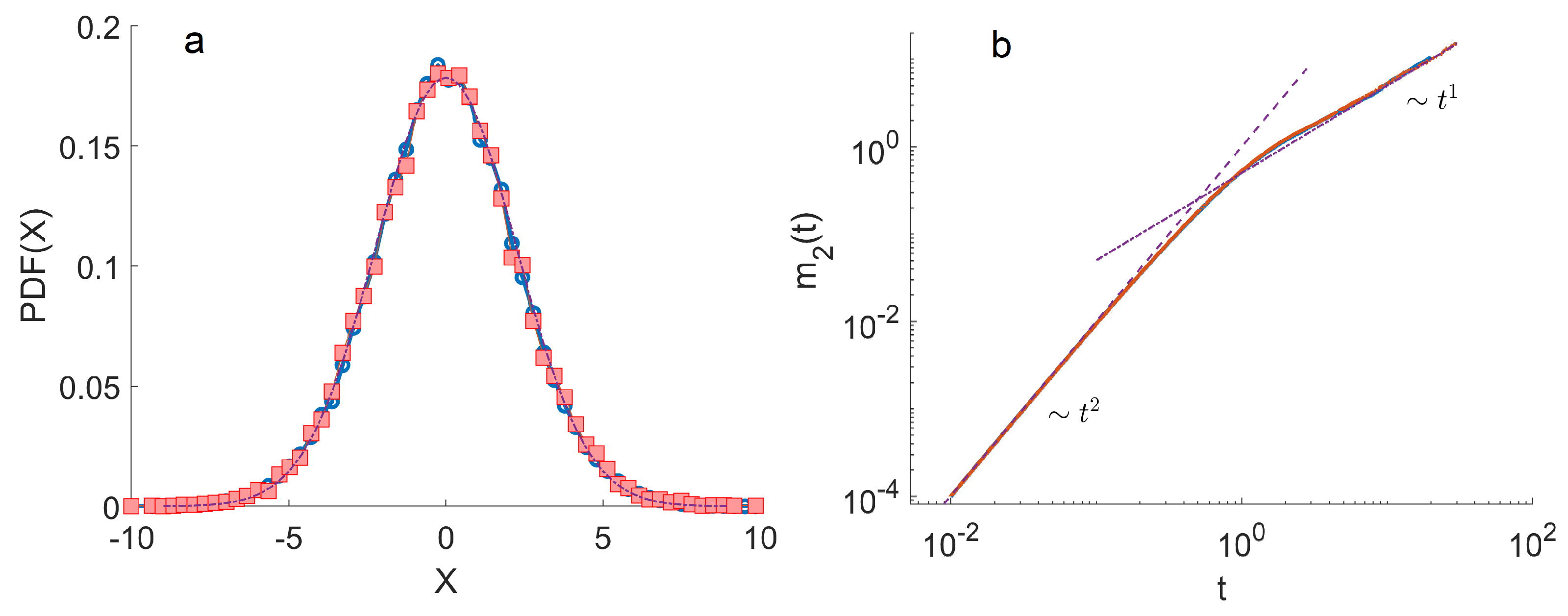
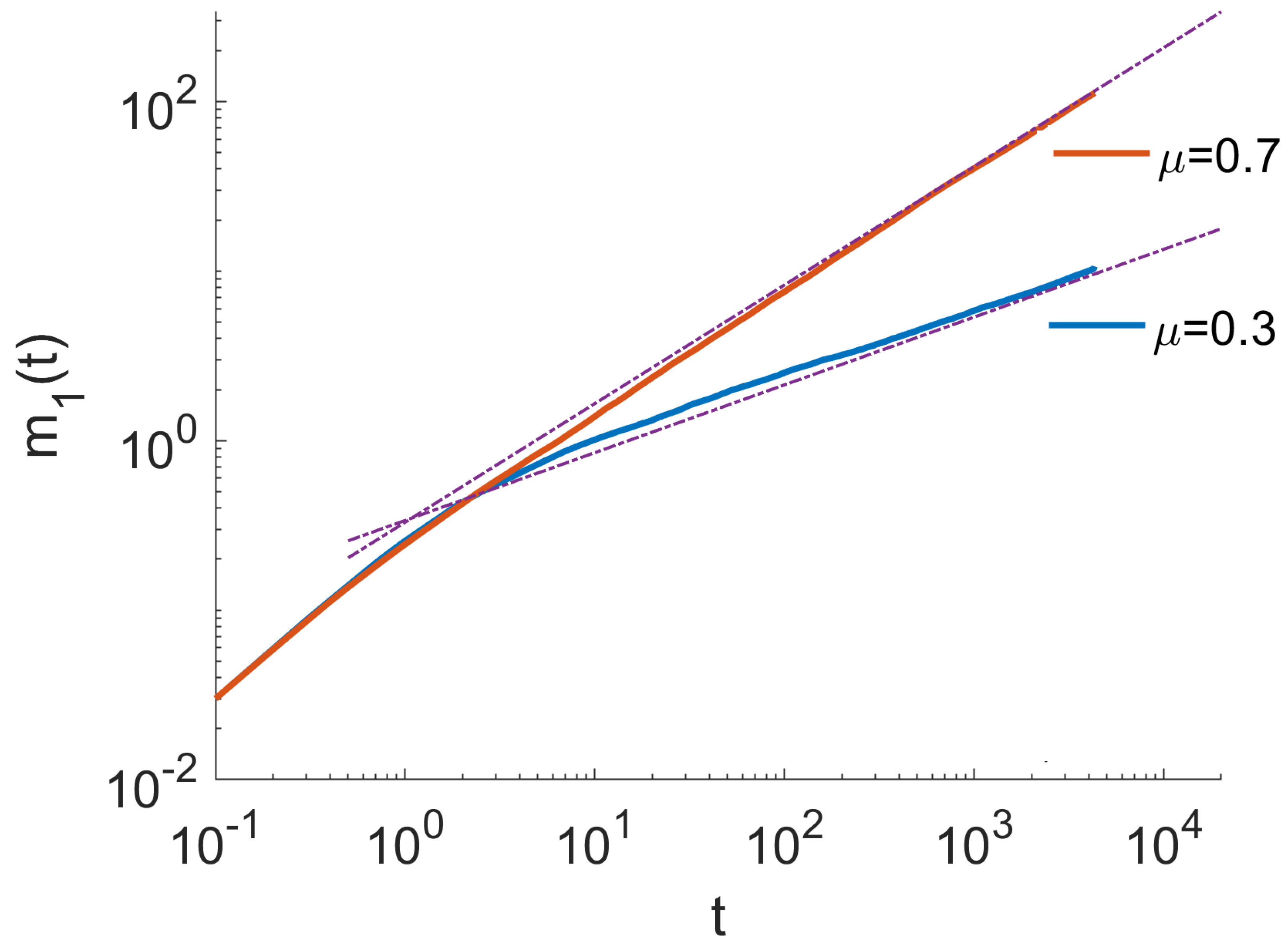
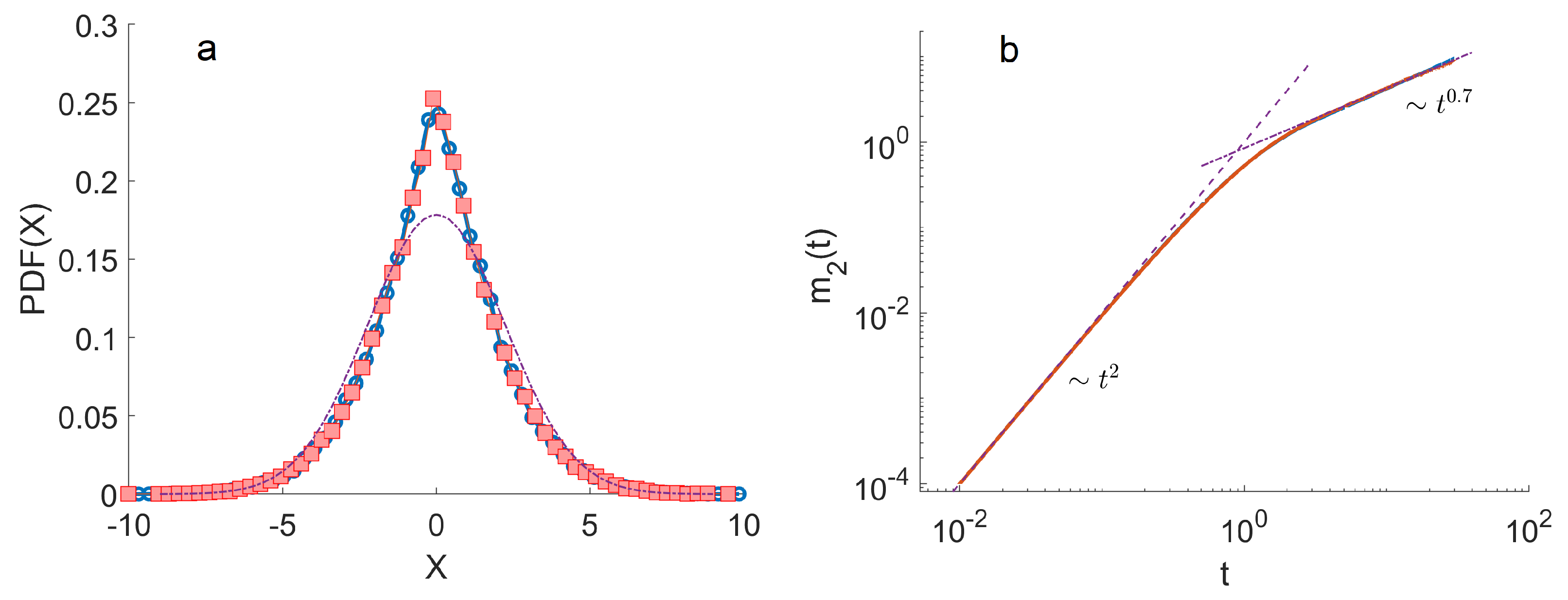
The ensemble of trajectories is then analysed by calculating the distribution of positions at a given $T_{max}$. We estimated these distributions using histograms. To quantify the anomalous diffusion in the Three-State Model, we calculated the moments of these distributions as a function of time. In particular, the first and the second moments were calculated as $m_1\left(t\right)={\sum }_{i=1}^N{x}^{\left(i\right)}\left(t\right)$, $m_2\left(t\right)={\sum }_{i=1}^N{\left(x^{\left(i\right)}\left(t\right)\right)}^2$. Here, $\left(i\right)$ denotes the index of a trajectory.

To achieve the simulation results for the Markovian Three-State Model, we compute the variance $m_2\left(t\right)-m_1^2\left(t\right)$ and distributions of walkers with parameters $\lambda =1$, $v_{+}=1$ and $v_{-}=1$. The results are shown in Figure 1. We chose equal probabilities of switching from resting to running state ${\gamma }_A={\gamma }_R={\gamma }_0=1/3$. As expected, the PDFs of the walker’s positions follow the Gaussian distribution. The corresponding second moments show ballistic regimes at short times and asymptotic linear growth.

For the Non-Markovian Three-State model, we also find good agreement with the theoretical predictions. First, we calculated the first moment $m_1\left(t\right)$ of random walker position as a function of time with zero removal rates $Q_A=Q_R=Q_0=0$, ${\lambda }_A={\lambda }_R=1/3$, ${\tau }_0=1$, $\lambda =1$ and $v_{+}=1,v_{-}=0.1$. We considered two values of anomalous exponent $\mu =0.3$ and $\mu =0.7$. As shown in Figure 2, the numerics agree with the analytical Equation (62) without fitting.

The ML-distributed resting states make the distributions of the walker’s position non-Gaussian. An example of the distributions of random walkers’ position with the resting states generated from the ML distribution with the scaling parameter $\mu =0.7$ is shown in Figure 3. At long times, the MSD is growing sub linearly with time, $m_2\left(t\right)\sim t^{\beta }$ with $\beta =\mu$. At the same time, it was previously found that the two-state model with one running state and the ML resting state has the long-time behaviour of the variance $m_2\left(t\right)-m_1^2\left(t\right)\sim t^{\beta }$ with $\beta =2\mu$. So, for $\mu <0.5$ the variance grows subdiffusively with time, and for $\mu >0.5$ the growth is superdiffusive.

We note that the two-state model is equivalent to the three-state model with the speed of one running state equal to zero. The following question arises: what would be the long-time behaviour of the three-state model with ML-distributed resting times with unequal retrograde and anterograde speeds? We calculated the variance of the position for the three-state model with ML-distributed resting times and showed that the model has subdiffusion or superdiffusion at long times depending on the parameters. At long times, the variance depends on cargo speeds and is well fitted by the power-law function:

$$m_2\left(t\right)-m_1^2\left(t\right)\sim t^{\beta },\beta =\mu \left(1+\frac{|v_{+}-v_{-}|}{v_{+}+v_{-}}\right).$$

(71)

For $v_{+}=v_{-}$, we recover the subdiffusive behaviour $\beta =\mu <1$ predicted by the Equation (70). The dependence of $\beta /\mu -1$ on the speed $v_{+}$ (with $v_{-}$ kept constant) for the three-state model with ML-distributed resting state is shown in Figure 4a. The asymptotic behaviour of different models given by the dependence of exponents of MSDs or variances at long times, $\beta$, is shown in Figure 4a. In contrast to the three-state model with equal retrograde and anterograde cargo speeds $v_{+}=v_{-}$, the three-state model with unequal retrograde and anterograde cargo speeds, $v_{+}\ne v_{-}$ can have subdiffusive behaviour and superdiffusive behaviour.

5. Discussion

In cells, vesicles are transported by dyneins from the cell periphery to the cell interior (retrograde transport) and kinesins transport them from the cell interior toward the cortex (anterograde transport). Dyneins and kinesins move at different velocities. Thus, in contrast to previous works [62,64], here, we considered different cargo velocities in retrograde and anterograde directions. As a result, the first moment of the cargo position $m_1\left(t\right)$ is non-zero but grows linearly with time for the Markovian model or as a power law in the case of the non-Markovian model. In experiments, this could be used to distinguish between Markovian and non-Markovian dynamics.

The variance of cargo position $m_2\left(t\right)-m_1^2\left(t\right)$ bears additional information about the cargo dynamics. For the non-Markovian model with unequal velocities, the variance can grow subdiffusively and superdiffusively depending on the anomalous exponent $\mu$ of the distribution of the duration of resting states. Combining predictions for the first moment, variance, and distribution of cargo’s displacements, it would be possible to verify the non-Markovian three-state model using the ensemble of experimental trajectories.

6. Summary and Conclusions

We have introduced a non-Markovian persistent random walk model for intracellular transport that incorporates the removal rate and finite speed of propagation. This model includes random transitions between two active states (anterograde and retrograde movements) and one resting state, with the probability of switching depending on the amount of time the organelle spends in each state. We have derived new mesoscopic integro-differential equations for densities of organelles inside the cell by using the structural densities obeying Markov differential equations of the first order. We have found a non-Markovian non-additivity effect when the switching rates and transport characteristics depend on the rate of organelles removal. Ordinary differential equations describing the dynamics for the first and second moments of the organelles’ position along the cell have been derived. A model of stochastic transport of organelles which takes into account experimentally observed Mittag-Leffler resting time distribution has been analysed in detail. In particular, it determines the subdiffusive and superdiffusive behaviour of the first moment. Notice that the fractional Riemann–Liouville derivative naturally arises as the result of the Mittag-Leffler distribution of residence times in the resting state. For a general form of resting time distribution, one should not expect the escape rate to be expressed with any kind of fractional derivative. Rather, it will be given by an integral form defined by Equation (34) A numerical Monte Carlo algorithm has been developed to calculate moments and organelle mesoscopic densities in cells, taking into account non-Markovian effects caused by the dependence of transition rates on residence times.

In this paper, we propose the mathematical model of intracellular transport. This model is based on experimental observations (see, for example [2,6]) that intracellular transport demonstrates so-called stop-and-go behaviour and is characterised by long time sub-diffusive behaviour. In this work, we modelled the stop-and-go behaviour as switching from active to resting states and showed that the ML distributed time spent in resting states leads to sub-diffusion at long times. So, experimentally, it would be possible to test the predictions of our model, e.g., whether the resting times are described by the ML distribution. In fact, in our previous work [27,57], we found that the distribution of resting times indeed might be better fitted by a power law (notice that the long-time asymptotic of the ML distribution is $t^{-1-\mu }$). However, more experimental data are needed to make this comparison more reliable.

In this paper, we used the assumption of constant cargo speeds. In experiments, intracellular organelles might be described based on the distribution of speed. Our constant speed assumption could be viewed as utilising the first moment of this distribution. In the future, it will be interesting to extend our work by taking into account the distribution of cargo speeds [51] and the heterogeneity of intracellular transport [24].

References

1. Brady, S.T.; Morfini, G.A. Regulation of motor proteins, axonal transport deficits and adult-onset neurodegenerative diseases. Neurobiol. Dis. 2017, 105, 273–282. [Google Scholar] [CrossRef] [PubMed]
2. Appert-Rolland, C.; Ebbinghaus, M.; Santen, L. Intracellular transport driven by cytoskeletal motors: General mechanisms and defects. Phys. Rep. 2015, 593, 1–59. [Google Scholar] [CrossRef]
3. Hancock, W.O. Bidirectional cargo transport: Moving beyond tug of war. Nat. Rev. Mol. Cell Biol. 2014, 15, 615–628. [Google Scholar] [CrossRef] [PubMed]
4. Schliwa, M.; Woehlke, G. Molecular motors. Nature 2003, 422, 759–765. [Google Scholar] [CrossRef]
5. Vale, R.D. The molecular motor toolbox for intracellular transport. Cell 2003, 112, 467–480. [Google Scholar] [CrossRef] [PubMed]
6. Hirokawa, N. Kinesin and dynein superfamily proteins and the mechanism of organelle transport. Science 1998, 279, 519–526. [Google Scholar] [CrossRef]
7. Allan, V. One, two, three, cytoplasmic dynein is go! Science 2014, 345, 271–272. [Google Scholar] [CrossRef]
8. Kardon, J.R.; Vale, R.D. Regulators of the cytoplasmic dynein motor. Nat. Rev. Mol. Cell Biol. 2009, 10, 854–865. [Google Scholar] [CrossRef]
9. Bressloff, P.C.; Newby, J.M. Stochastic models of intracellular transport. Rev. Mod. Phys. 2013, 85, 135. [Google Scholar] [CrossRef]
10. Briane, V.; Vimond, M.; Kervrann, C. An overview of diffusion models for intracellular dynamics analysis. Briefings Bioinform. 2020, 21, 1136–1150. [Google Scholar] [CrossRef]
11. Smith, D.A.; Simmons, R.M. Models of motor-assisted transport of intracellular particles. Biophys. Journal 2001, 80, 45–68. [Google Scholar] [CrossRef]
12. Bressloff, P.C. Stochastic Processes in Cell Biology; Springer: Berlin/Heidelberg, Germany, 2014; Volume 41. [Google Scholar]
13. Jülicher, F.; Ajdari, A.; Prost, J. Modeling molecular motors. Rev. Mod. Phys. 1997, 69, 1269. [Google Scholar] [CrossRef]
14. Klumpp, S.; Lipowsky, R. Cooperative cargo transport by several molecular motors. Proc. Natl. Acad. Sci. USA 2005, 102, 17284–17289. [Google Scholar] [CrossRef] [PubMed]
15. Hafner, A.E.; Santen, L.; Rieger, H.; Shaebani, M.R. Run-and-pause dynamics of cytoskeletal motor proteins. Sci. Rep. 2016, 6, 37162. [Google Scholar] [CrossRef] [PubMed]
16. Loverdo, C.; Bénichou, O.; Moreau, M.; Voituriez, R. Enhanced reaction kinetics in biological cells. Nat. Phys. 2008, 4, 134–137. [Google Scholar] [CrossRef]
17. Newby, J.; Bressloff, P.C. Random intermittent search and the tug-of-war model of motor-driven transport. J. Stat. Mech. Theory Exp. 2010, 2010, P04014. [Google Scholar] [CrossRef]
18. Chou, T.; Mallick, K.; Zia, R.K. Non-equilibrium statistical mechanics: From a paradigmatic model to biological transport. Rep. Prog. Phys. 2011, 74, 116601. [Google Scholar] [CrossRef]
19. Schadschneider, A.; Chowdhury, D.; Nishinari, K. Stochastic Transport in Complex Systems: From Molecules to Vehicles; Elsevier: Amsterdam, The Netherlands, 2010. [Google Scholar]
20. Pinkoviezky, I.; Gov, N. Transport dynamics of molecular motors that switch between an active and inactive state. Phys. Rev. E 2013, 88, 022714. [Google Scholar] [CrossRef]
21. Ando, D.; Korabel, N.; Huang, K.C.; Gopinathan, A. Cytoskeletal network morphology regulates intracellular transport dynamics. Biophys. J. 2015, 109, 1574–1582. [Google Scholar] [CrossRef]
22. Hafner, A.E.; Rieger, H. Spatial cytoskeleton organization supports targeted intracellular transport. Biophys. J. 2018, 114, 1420–1432. [Google Scholar] [CrossRef]
23. Cherstvy, A.G.; Chechkin, A.V.; Metzler, R. Particle invasion, survival, and non-ergodicity in 2D diffusion processes with space-dependent diffusivity. Soft Matter. 2014, 10, 1591–1601. [Google Scholar] [CrossRef] [PubMed]
24. Korabel, N.; Taloni, A.; Pagnini, G.; Allan, V.; Fedotov, S.; Waigh, T.A. Ensemble heterogeneity mimics ageing for endosomal dynamics within eukaryotic cells. Sci. Rep. 2023, 13, 8789. [Google Scholar] [CrossRef] [PubMed]
25. Shaebani, M.R.; Sadjadi, Z.; Sokolov, I.M.; Rieger, H.; Santen, L. Anomalous diffusion of self-propelled particles in directed random environments. Phys. Rev. E 2014, 90, 030701. [Google Scholar] [CrossRef] [PubMed]
26. Klein, S.; Appert-Rolland, C.; Santen, L. Fluctuation effects in bidirectional cargo transport. Eur. Phys. J. Spec. Top. 2014, 223, 3215–3225. [Google Scholar] [CrossRef]
27. Korabel, N.; Waigh, T.A.; Fedotov, S.; Allan, V.J. Non-Markovian intracellular transport with sub-diffusion and run-length dependent detachment rate. PLoS ONE 2018, 13, e0207436. [Google Scholar] [CrossRef]
28. Doerries, T.J.; Metzler, R.; Chechkin, A.V. Emergent anomalous transport and non-Gaussianity in a simple mobile–immobile model: The role of advection. New J. Phys. 2023, 25, 063009. [Google Scholar] [CrossRef]
29. Doerries, T.J.; Chechkin, A.V.; Schumer, R.; Metzler, R. Rate equations, spatial moments, and concentration profiles for mobile-immobile models with power-law and mixed waiting time distributions. Phys. Rev. E 2022, 105, 014105. [Google Scholar] [CrossRef]
30. Kurilovich, A.A.; Mantsevich, V.N.; Mardoukhi, Y.; Stevenson, K.J.; Chechkin, A.V.; Palyulin, V.V. Non-Markovian diffusion of excitons in layered perovskites and transition metal dichalcogenides. Phys. Chem. Chem. Phys. 2022, 24, 13941–13950. [Google Scholar] [CrossRef]
31. Bouchaud, J.P.; Georges, A. Anomalous diffusion in disordered media: Statistical mechanisms, models and physical applications. Phys. Rep. 1990, 195, 127–293. [Google Scholar] [CrossRef]
32. Metzler, R.; Klafter, J. The random walk’s guide to anomalous diffusion: A fractional dynamics approach. Phys. Rep. 2000, 339, 1–77. [Google Scholar] [CrossRef]
33. Metzler, R.; Klafter, J. The restaurant at the end of the random walk: Recent developments in the description of anomalous transport by fractional dynamics. J. Phys. Math. Gen. 2004, 37, R161. [Google Scholar] [CrossRef]
34. Barkai, E.; Garini, Y.; Metzler, R. Strange kinetics of single molecules in living cells. Phys. Today 2012, 65, 29–35. [Google Scholar] [CrossRef]
35. Waigh, T.A. The Physics of Living Processes: A Mesoscopic Approach; John Wiley & Sons: Hoboken, NJ, USA, 2014. [Google Scholar]
36. Zaburdaev, V.; Denisov, S.; Klafter, J. Lévy walks. Rev. Mod. Phys. 2015, 87, 483. [Google Scholar] [CrossRef]
37. Metzler, R.; Jeon, J.H.; Cherstvy, A.G.; Barkai, E. Anomalous diffusion models and their properties: Non-stationarity, non-ergodicity, and ageing at the centenary of single particle tracking. Phys. Chem. Chem. Phys. 2014, 16, 24128–24164. [Google Scholar] [CrossRef] [PubMed]
38. Waigh, T.A.; Korabel, N. Heterogeneous anomalous transport in cellular and molecular biology. Rep. Prog. Phys. 2023; in press. [Google Scholar]
39. Salman, H.; Gil, Y.; Granek, R.; Elbaum, M. Microtubules, motor proteins, and anomalous mean squared displacements. Chem. Phys. 2002, 284, 389–397. [Google Scholar] [CrossRef]
40. Caspi, A.; Granek, R.; Elbaum, M. Diffusion and directed motion in cellular transport. Phys. Rev. E 2002, 66, 011916. [Google Scholar] [CrossRef]
41. Weiss, M.; Elsner, M.; Kartberg, F.; Nilsson, T. Anomalous subdiffusion is a measure for cytoplasmic crowding in living cells. Biophys. J. 2004, 87, 3518–3524. [Google Scholar] [CrossRef]
42. Kulkarni, R.P.; Castelino, K.; Majumdar, A.; Fraser, S.E. Intracellular transport dynamics of endosomes containing DNA polyplexes along the microtubule network. Biophys. J. 2006, 90, L42–L44. [Google Scholar] [CrossRef]
43. Kulić, I.M.; Brown, A.E.; Kim, H.; Kural, C.; Blehm, B.; Selvin, P.R.; Nelson, P.C.; Gelfand, V.I. The role of microtubule movement in bidirectional organelle transport. Proc. Natl. Acad. Sci. USA 2008, 105, 10011–10016. [Google Scholar] [CrossRef]
44. Bruno, L.; Levi, V.; Brunstein, M.; Desposito, M.A. Transition to superdiffusive behavior in intracellular actin-based transport mediated by molecular motors. Phys. Rev. E 2009, 80, 011912. [Google Scholar] [CrossRef] [PubMed]
45. Robert, D.; Nguyen, T.H.; Gallet, F.; Wilhelm, C. In vivo determination of fluctuating forces during endosome trafficking using a combination of active and passive microrheology. PLoS ONE 2010, 5, e10046. [Google Scholar] [CrossRef] [PubMed]
46. Tabei, S.A.; Burov, S.; Kim, H.Y.; Kuznetsov, A.; Huynh, T.; Jureller, J.; Philipson, L.H.; Dinner, A.R.; Scherer, N.F. Intracellular transport of insulin granules is a subordinated random walk. Proc. Natl. Acad. Sci. USA 2013, 110, 4911–4916. [Google Scholar] [CrossRef] [PubMed]
47. Chen, K.; Wang, B.; Granick, S. Memoryless self-reinforcing directionality in endosomal active transport within living cells. Nat. Mater. 2015, 14, 589–593. [Google Scholar] [CrossRef]
48. Reverey, J.F.; Jeon, J.H.; Bao, H.; Leippe, M.; Metzler, R.; Selhuber-Unkel, C. Superdiffusion dominates intracellular particle motion in the supercrowded cytoplasm of pathogenic Acanthamoeba castellanii. Sci. Rep. 2015, 5, 11690. [Google Scholar] [CrossRef]
49. Song, M.S.; Moon, H.C.; Jeon, J.H.; Park, H.Y. Neuronal messenger ribonucleoprotein transport follows an aging Lévy walk. Nat. Commun. 2018, 9, 344. [Google Scholar] [CrossRef]
50. Flores-Rodriguez, N.; Rogers, S.S.; Kenwright, D.A.; Waigh, T.A.; Woodman, P.G.; Allan, V.J. Roles of dynein and dynactin in early endosome dynamics revealed using automated tracking and global analysis. PLoS ONE 2011, 6, e24479. [Google Scholar] [CrossRef]
51. Han, D.; Korabel, N.; Chen, R.; Johnston, M.; Gavrilova, A.; Allan, V.J.; Fedotov, S.; Waigh, T.A. Deciphering anomalous heterogeneous intracellular transport with neural networks. Elife 2020, 9, e52224. [Google Scholar] [CrossRef]
52. Korabel, N.; Han, D.; Taloni, A.; Pagnini, G.; Fedotov, S.; Allan, V.; Waigh, T.A. Local analysis of heterogeneous intracellular transport: Slow and fast moving endosomes. Entropy 2021, 23, 958. [Google Scholar] [CrossRef]
53. Banks, D.S.; Fradin, C. Anomalous diffusion of proteins due to molecular crowding. Biophys. J. 2005, 89, 2960–2971. [Google Scholar] [CrossRef]
54. Weiss, M. Crowding, diffusion, and biochemical reactions. Int. Rev. Cell Mol. Biol. 2014, 307, 383–417. [Google Scholar] [PubMed]
55. Waigh, T.A. Microrheology of complex fluids. Rep. Prog. Phys. 2005, 68, 685. [Google Scholar] [CrossRef]
56. Waigh, T.A. Advances in the microrheology of complex fluids. Rep. Prog. Phys. 2016, 79, 074601. [Google Scholar] [CrossRef] [PubMed]
57. Fedotov, S.; Korabel, N.; Waigh, T.A.; Han, D.; Allan, V.J. Memory effects and Lévy walk dynamics in intracellular transport of cargoes. Phys. Rev. E 2018, 98, 042136. [Google Scholar] [CrossRef]
58. Zumofen, G.; Klafter, J. Laminar–localized-phase coexistence in dynamical systems. Phys. Rev. E 1995, 51, 1818. [Google Scholar] [CrossRef]
59. Thiel, F.; Schimansky-Geier, L.; Sokolov, I.M. Anomalous diffusion in run-and-tumble motion. Phys. Rev. E 2012, 86, 021117. [Google Scholar] [CrossRef]
60. Portillo, I.G.; Campos, D.; Méndez, V. Intermittent random walks: Transport regimes and implications on search strategies. J. Stat. Mech. Theory Exp. 2011, 2011, P02033. [Google Scholar] [CrossRef]
61. Klafter, J.; Sokolov, I.M. First Steps in Random Walks: From Tools to Applications; OUP Oxford: Oxford, UK, 2011. [Google Scholar]
62. Han, D.; Alexandrov, D.V.; Gavrilova, A.; Fedotov, S. Anomalous stochastic transport of particles with self-reinforcement and mittag–leffler distributed rest times. Fractal Fract. 2021, 5, 221. [Google Scholar] [CrossRef]
63. Fedotov, S.; Han, D.; Ivanov, A.O.; Da Silva, M.A. Superdiffusion in self-reinforcing run-and-tumble model with rests. Phys. Rev. E 2022, 105, 014126. [Google Scholar] [CrossRef]
64. Al Shamsi, H. Migration and Proliferation Dichotomy: A Persistent Random Walk of Cancer Cells. Fractal Fract. 2023, 7, 318. [Google Scholar] [CrossRef]
65. Vlad, M.O.; Ross, J. Systematic derivation of reaction-diffusion equations with distributed delays and relations to fractional reaction-diffusion equations and hyperbolic transport equations: Application to the theory of Neolithic transition. Phys. Rev. E 2002, 66, 061908. [Google Scholar] [CrossRef]
66. Mendez, V.; Fedotov, S.; Horsthemke, W. Reaction-Transport Systems: Mesoscopic Foundations, Fronts, and Spatial Instabilities; Springer Science & Business Media: Berlin/Heidelberg, Germany, 2010. [Google Scholar]
67. Fedotov, S. Single integrodifferential wave equation for a Lévy walk. Phys. Rev. E 2016, 93, 020101. [Google Scholar] [CrossRef] [PubMed]
68. Giona, M.; Cairoli, A.; Klages, R. Extended Poisson-Kac theory: A unifying framework for stochastic processes with finite propagation velocity. Phys. Rev. X 2022, 12, 021004. [Google Scholar] [CrossRef]
69. Cox, D.R.; Miller, H.D. The theory of Stochastic Processes; Routledge: Cambridge, MA, USA, 2017. [Google Scholar]
70. Fedotov, S.; Al-Shamsi, H.; Ivanov, A.; Zubarev, A. Anomalous transport and nonlinear reactions in spiny dendrites. Phys. Rev. E 2010, 82, 041103. [Google Scholar] [CrossRef] [PubMed]
71. Henry, B.; Langlands, T.; Wearne, S. Anomalous diffusion with linear reaction dynamics: From continuous time random walks to fractional reaction-diffusion equations. Phys. Rev. E 2006, 74, 031116. [Google Scholar] [CrossRef] [PubMed]
72. Angstmann, C.N.; Donnelly, I.C.; Henry, B.I. Continuous time random walks with reactions forcing and trapping. Math. Model. Nat. Phenom. 2013, 8, 17–27. [Google Scholar] [CrossRef]
73. Fedotov, S.; Iomin, A.; Ryashko, L. Non-Markovian models for migration-proliferation dichotomy of cancer cells: Anomalous switching and spreading rate. Phys. Rev. E 2011, 84, 061131. [Google Scholar] [CrossRef]
74. Böttger, K.; Hatzikirou, H.; Chauviere, A.; Deutsch, A. Investigation of the migration/proliferation dichotomy and its impact on avascular glioma invasion. Math. Model. Nat. Phenom. 2012, 7, 105–135. [Google Scholar] [CrossRef]
75. Iomin, A. Continuous time random walk and migration–proliferation dichotomy of brain cancer. Biophys. Rev. Lett. 2015, 10, 37–57. [Google Scholar] [CrossRef]
76. Pogorui, A.A.; Rodríguez-Dagnino, R.M. Isotropic random motion at finite speed with K-Erlang distributed direction alternations. J. Stat. Phys. 2011, 145, 102–112. [Google Scholar] [CrossRef]
77. Taylor-King, J.P.; Klages, R.; Fedotov, S.; Van Gorder, R.A. Fractional diffusion equation for an n-dimensional correlated Lévy walk. Phys. Rev. E 2016, 94, 012104. [Google Scholar] [CrossRef] [PubMed]
78. Santra, I.; Basu, U.; Sabhapandit, S. Run-and-tumble particles in two dimensions: Marginal position distributions. Phys. Rev. E 2020, 101, 062120. [Google Scholar] [CrossRef] [PubMed]
79. Di Crescenzo, A.; Iuliano, A.; Mustaro, V. On some finite-velocity random motions driven by the geometric counting process. J. Stat. Phys. 2023, 190, 44. [Google Scholar] [CrossRef]
Figure 1. Markovian three–state model. (a) The distribution of random walkers is calculated at T m a x = 10 with zero removal rates Q A = Q R = Q 0 = 0 (circles) and Q A = Q R = Q 0 = 0.1 (squares). Other parameters are given in the text. The dashed line represents the Gaussian distribution with σ 2 = 2 D T m a x . (b) The corresponding second moment m 2 ( t ) as a function of time (blue and red curves) grows ballistically for short times and switches to linear growth with the effective diffusion coefficient D.
Fractalfract 07 00758 g001
Figure 2. Non–Markovian three–state model. The first moment m 1 ( t ) of random walkers position as a function of time calculated with zero removal rates Q A = Q R = Q 0 = 0 , λ A = λ R = λ 0 = 1 / 3 , μ = 0.3 , μ = 0.7 , τ 0 = 1 , λ = 1 and v + = 1 , v = 0.1 . The dashed lines correspond to the analytical Equation (62) without fitting.
Fractalfract 07 00758 g002
Figure 3. Non–Markovian three–state model. (a) The distribution of random walkers is calculated at T m a x = 10 with zero removal rates Q A = Q R = Q 0 = 0 (circles) and Q A = Q R = Q 0 = 0.1 (squares), τ 0 = 1 , λ = 1 and v + = 1 , v = 0.1 . The dashed line shows the Gaussian distribution for comparison. (b) The corresponding mean squared displacements (blue and red curves) grow ballistically for short times and switch to sub-linear growth m 2 ( t ) t β with β = μ and the exponent μ = 0.7 .
Fractalfract 07 00758 g003
Figure 4. Three–state model with ML–distributed resting times can have subdiffusive or superdiffusive asymptotic behaviour. (a) The dependence β / μ 1 as a function of the speed v + (with v kept constant) for the three-state model with ML-distributed resting state. The dashed line corresponds to Equation (71) and symbols show the results of numerical simulations. (b) The diagram of the asymptotic behaviour of different models is given by the dependence of exponents of MSDs or variances at long times, β , as functions of the exponent of ML distribution of resting states, μ . The line with the biggest slope corresponds to the two-state model (that is, the three-state model with either v + = 0 or v = 0 ) with ML-distributed resting states. It has subdiffusive behaviour β < 1 for μ < 1 / 2 and superdiffusive behaviour β > 1 for μ > 1 / 2 . The lowest line corresponds to the three-state model with equal retrograde and anterograde cargo speeds v + = v . The line with an intermediate slope corresponds to the three-state model with unequal retrograde and anterograde cargo speeds, v + = 1 and v = 0.25 .
Fractalfract 07 00758 g004
Disclaimer/Publisher’s Note: The statements, opinions and data contained in all publications are solely those of the individual author(s) and contributor(s) and not of MDPI and/or the editor(s). MDPI and/or the editor(s) disclaim responsibility for any injury to people or property resulting from any ideas, methods, instructions or products referred to in the content.