Figure 1.
Fractional-order Zener model.
Figure 1.
Fractional-order Zener model.
Figure 2.
A single-degree-of-freedom fractional Zener VE damper system.
Figure 2.
A single-degree-of-freedom fractional Zener VE damper system.
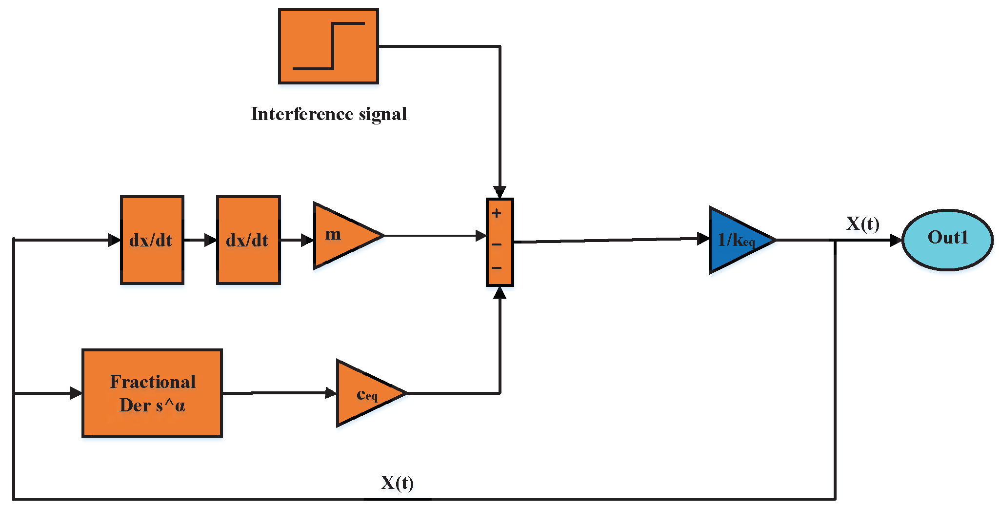
Figure 3.
Simulink block diagram for the fractional equation with zero initial values.
Figure 3.
Simulink block diagram for the fractional equation with zero initial values.
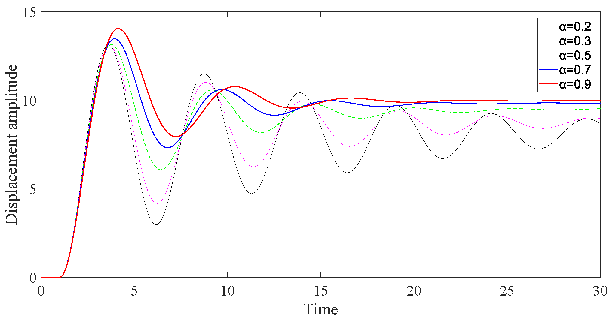
Figure 4.
Vibration responses of the fractional Zener VE damper with different fractional order .
Figure 4.
Vibration responses of the fractional Zener VE damper with different fractional order .
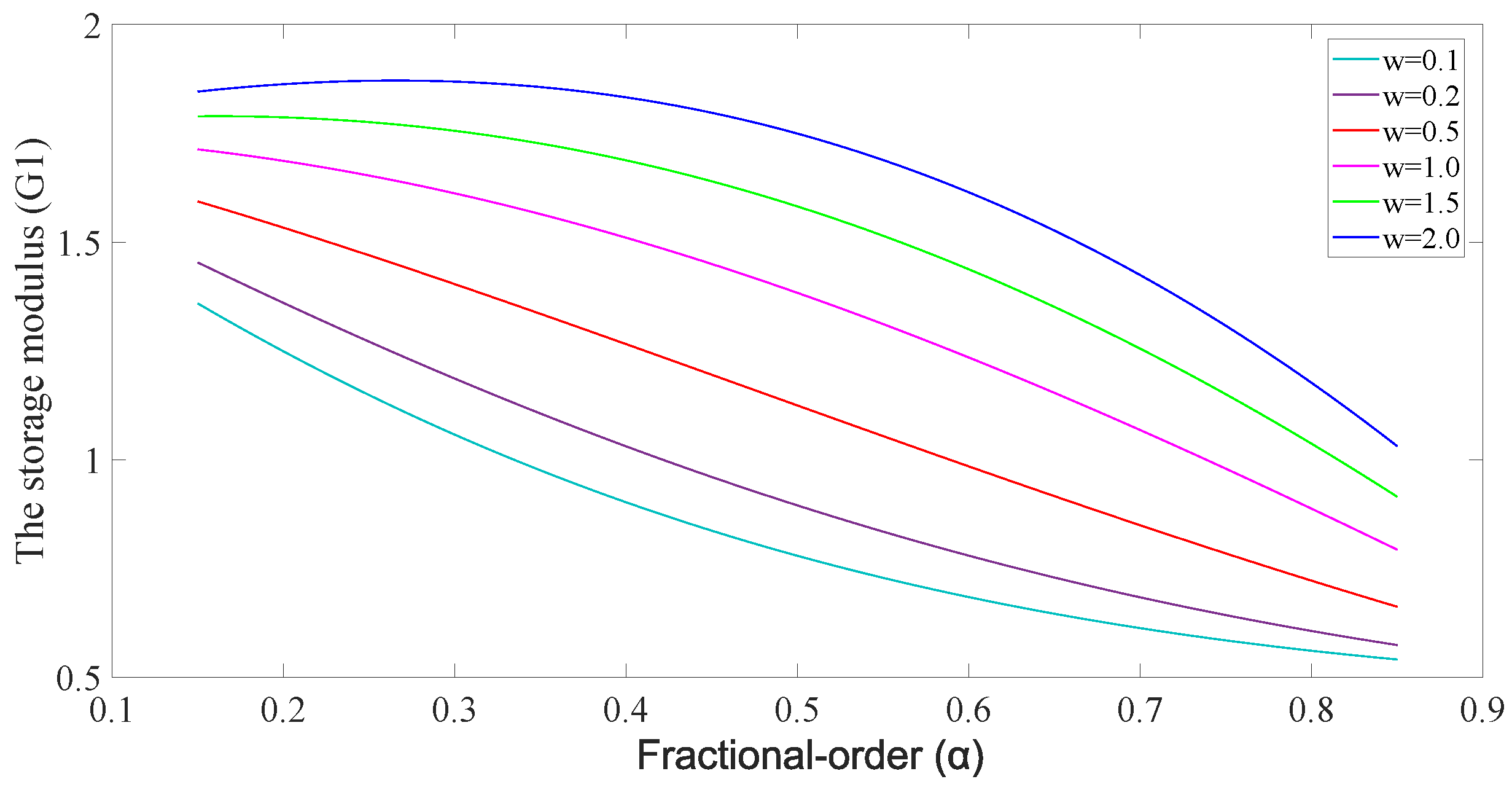
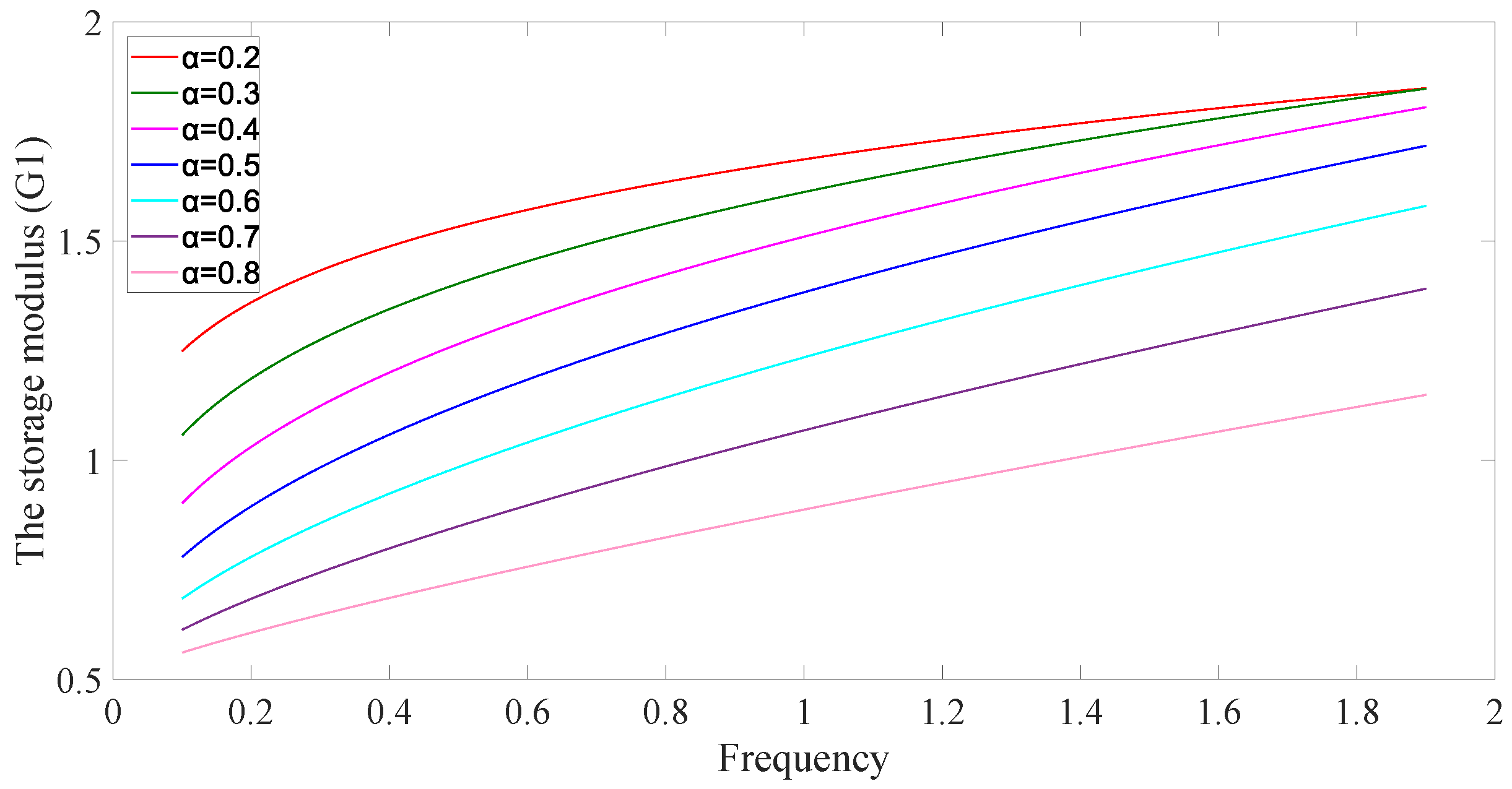
Figure 5.
The storage modulus of the VE damper at different frequencies and fractional orders.
Figure 5.
The storage modulus of the VE damper at different frequencies and fractional orders.
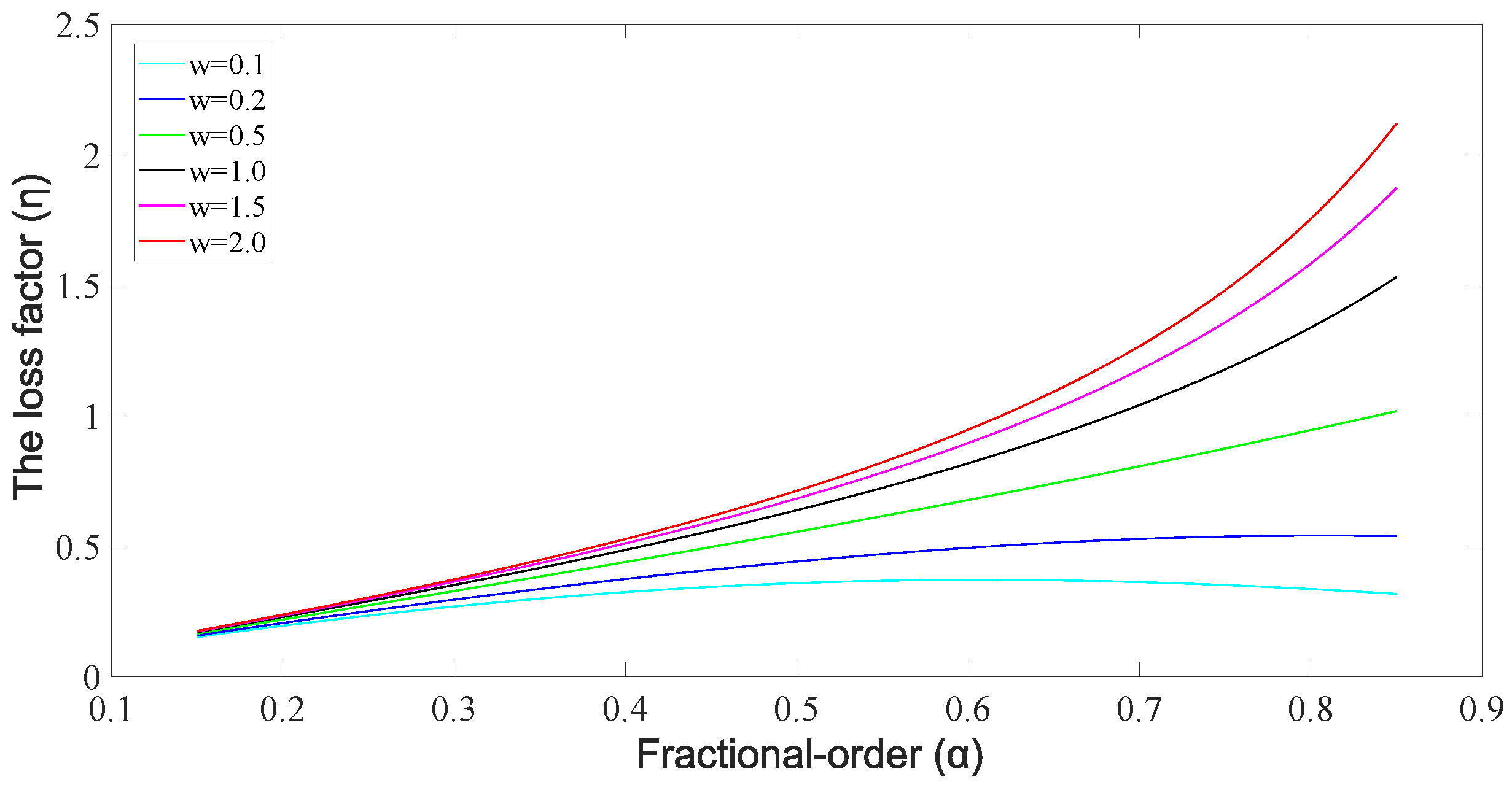
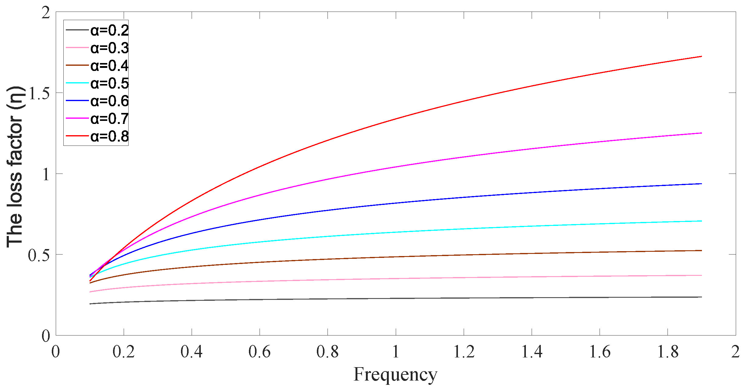
Figure 6.
The loss factor of the VE damper at different frequencies and fractional orders.
Figure 6.
The loss factor of the VE damper at different frequencies and fractional orders.
Figure 7.
The storage modulus of the VE damper at different fractional orders and frequencies.
Figure 7.
The storage modulus of the VE damper at different fractional orders and frequencies.
Figure 8.
The loss factor of the VE damper at different fractional orders and frequencies.
Figure 8.
The loss factor of the VE damper at different fractional orders and frequencies.
Figure 9.
The loss factor of the VE damper at different temperatures.
Figure 9.
The loss factor of the VE damper at different temperatures.
Figure 10.
The storage modulus of the VE damper at different temperatures.
Figure 10.
The storage modulus of the VE damper at different temperatures.
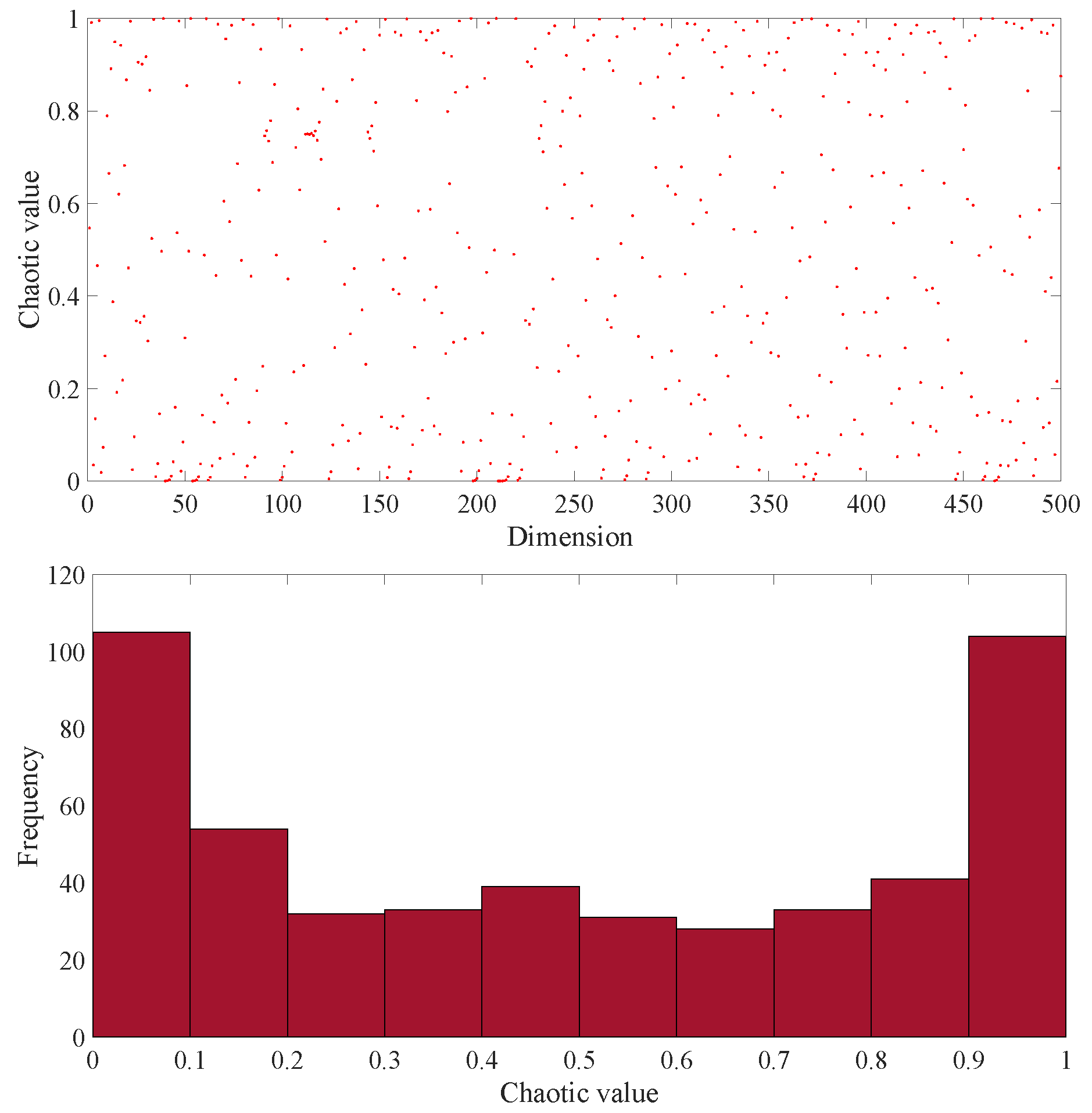
Figure 11.
Chaotic mapping generating chaotic numbers.
Figure 11.
Chaotic mapping generating chaotic numbers.
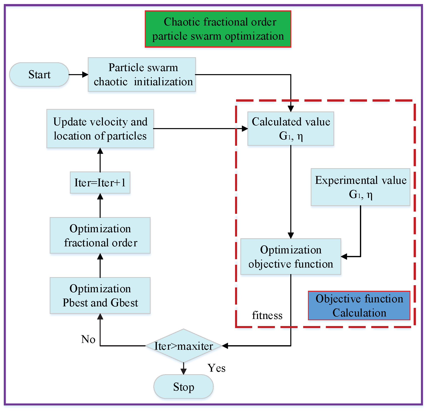
Figure 12.
Flowchart of the CFOPSO algorithm.
Figure 12.
Flowchart of the CFOPSO algorithm.
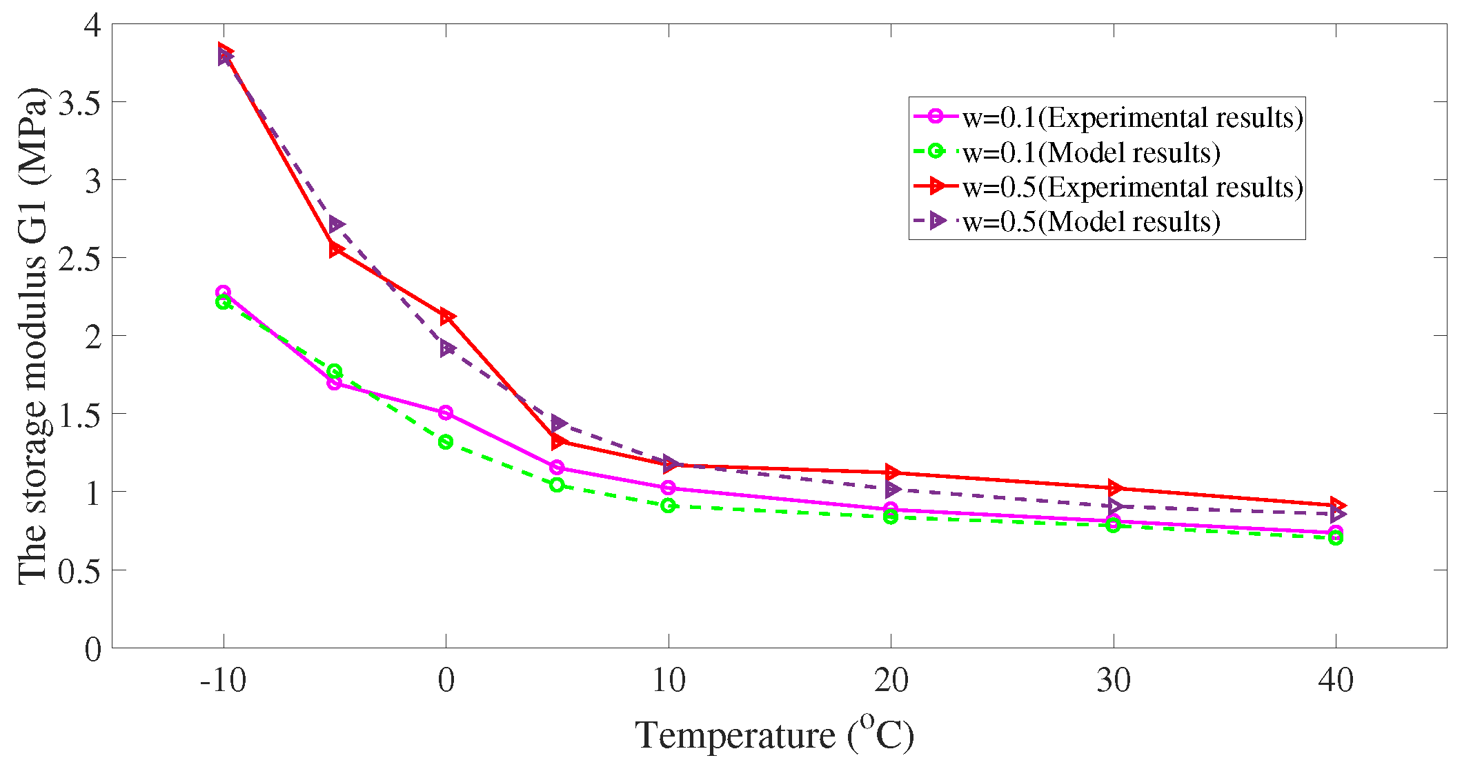
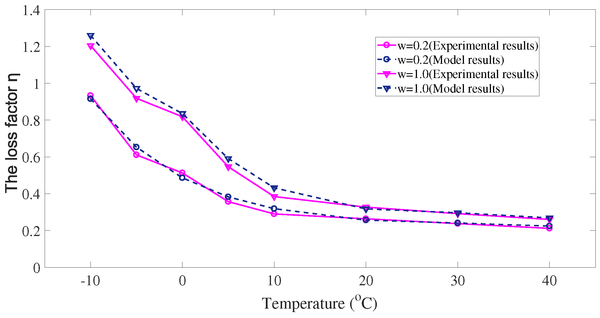
Figure 13.
Comparison between numerical and experimental results of ().
Figure 13.
Comparison between numerical and experimental results of ().
Figure 14.
Comparison between numerical and experimental results of ().
Figure 14.
Comparison between numerical and experimental results of ().
Figure 15.
Comparison between numerical and experimental results of ().
Figure 15.
Comparison between numerical and experimental results of ().
Figure 16.
Comparison between numerical and experimental results of ().
Figure 16.
Comparison between numerical and experimental results of ().
Figure 17.
Comparison between numerical and experimental results of with 40 when mm and rad/s.
Figure 17.
Comparison between numerical and experimental results of with 40 when mm and rad/s.
Figure 18.
Comparison between numerical and experimental results of with 40 when mm and rad/s.
Figure 18.
Comparison between numerical and experimental results of with 40 when mm and rad/s.
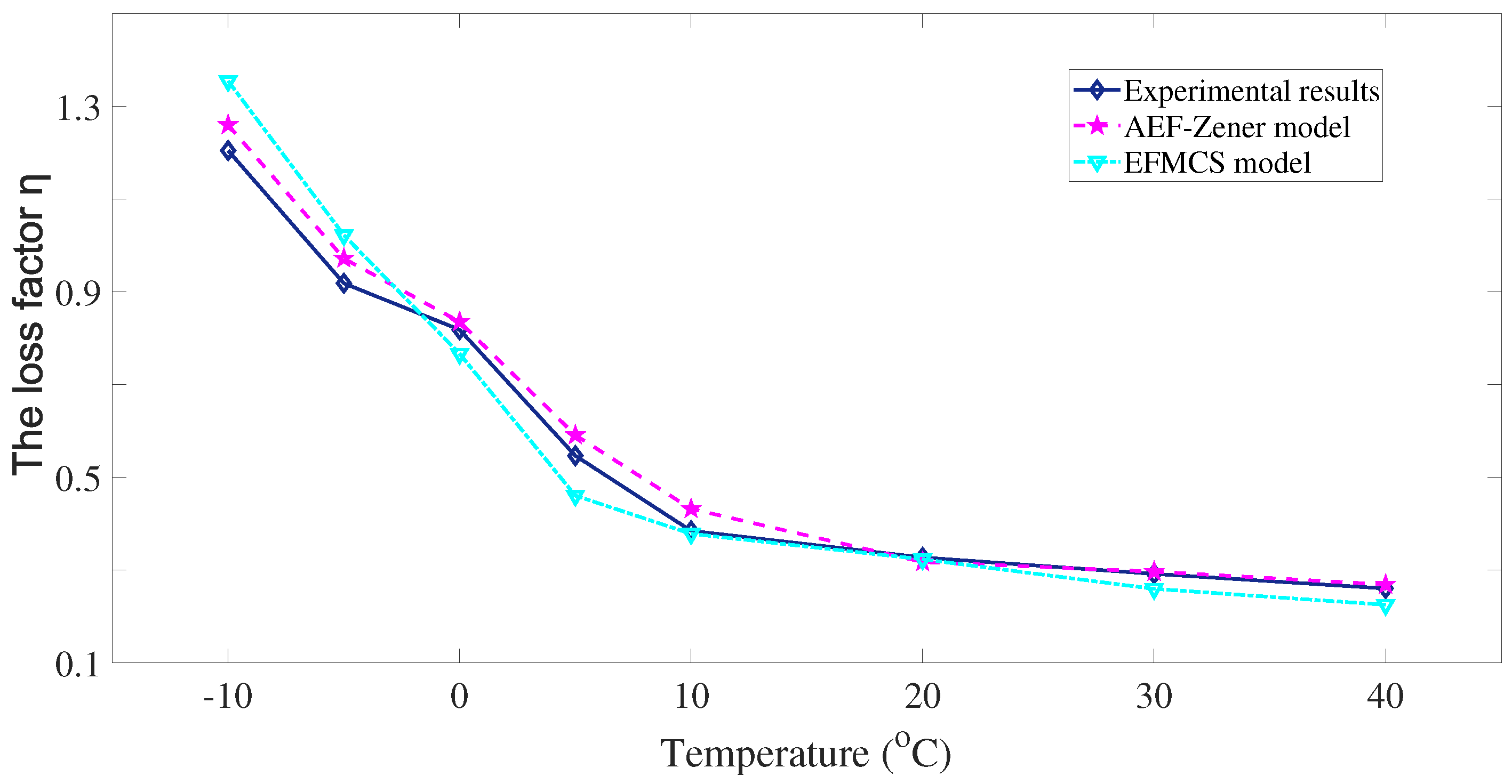
Figure 19.
Comparison of numerical and experimental results of with when mm and .
Figure 19.
Comparison of numerical and experimental results of with when mm and .
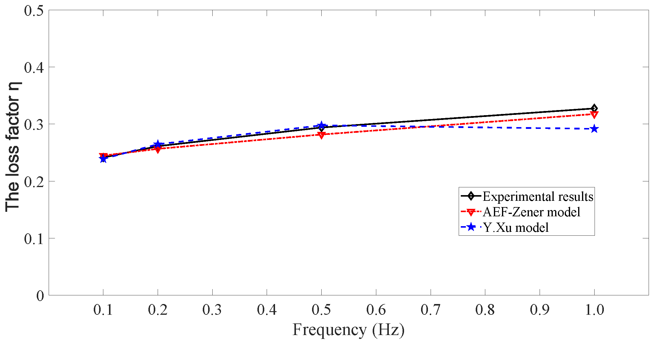
Figure 20.
Comparison of numerical and experimental results of with , when mm and .
Figure 20.
Comparison of numerical and experimental results of with , when mm and .
Figure 21.
El-Centro and Taft earthquake seismic waves.
Figure 21.
El-Centro and Taft earthquake seismic waves.
Figure 22.
A three-story building with VE dampers.
Figure 22.
A three-story building with VE dampers.
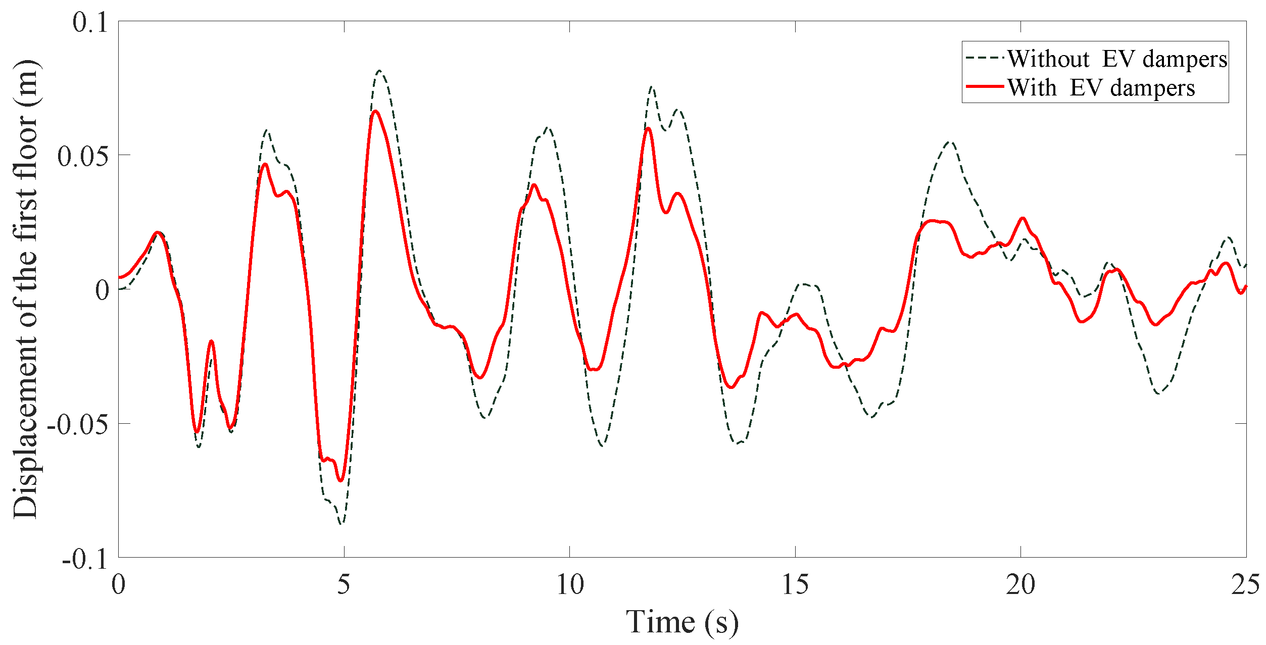
Figure 23.
First floor displacement of the building in the example in the El Centro earthquake.
Figure 23.
First floor displacement of the building in the example in the El Centro earthquake.
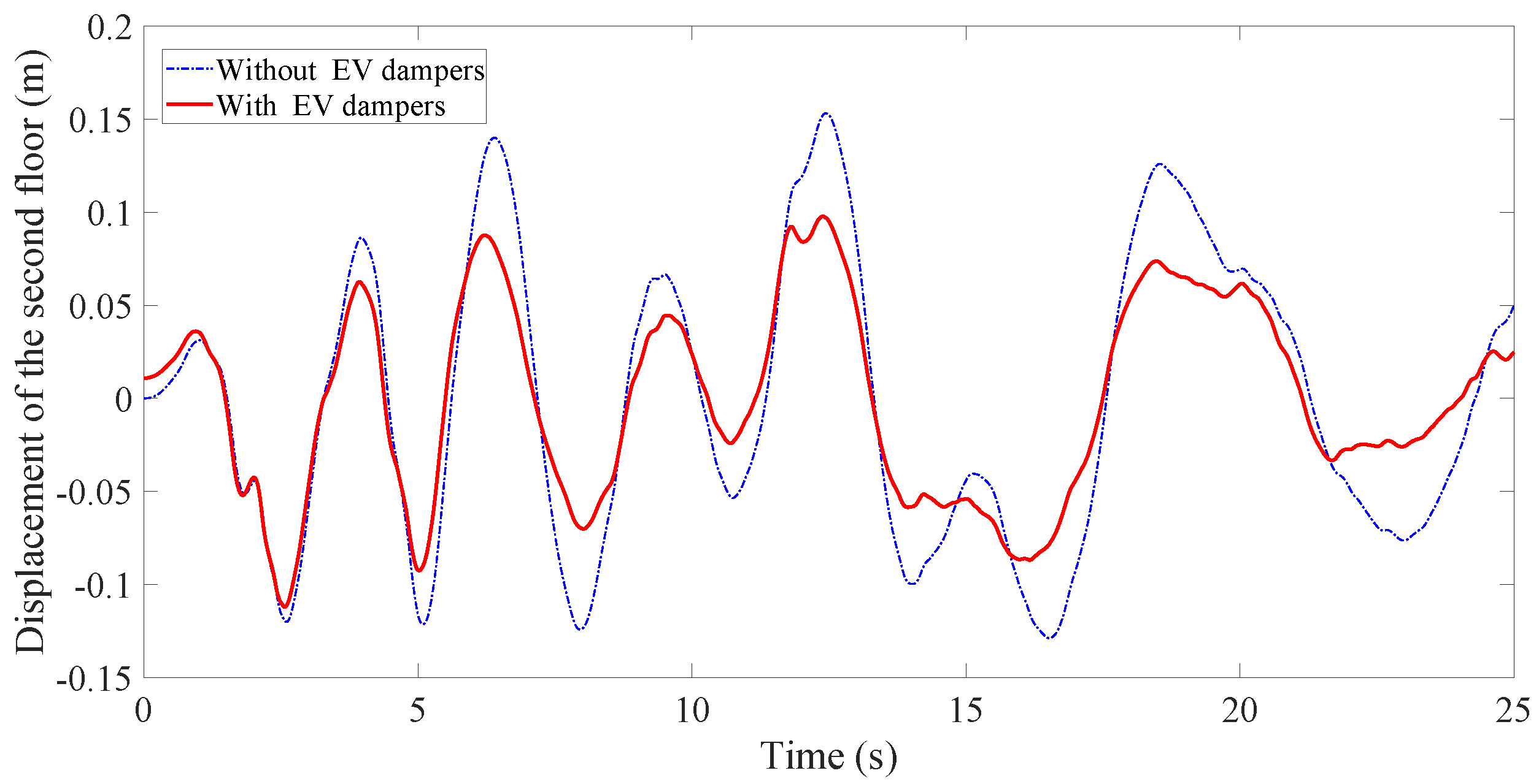
Figure 24.
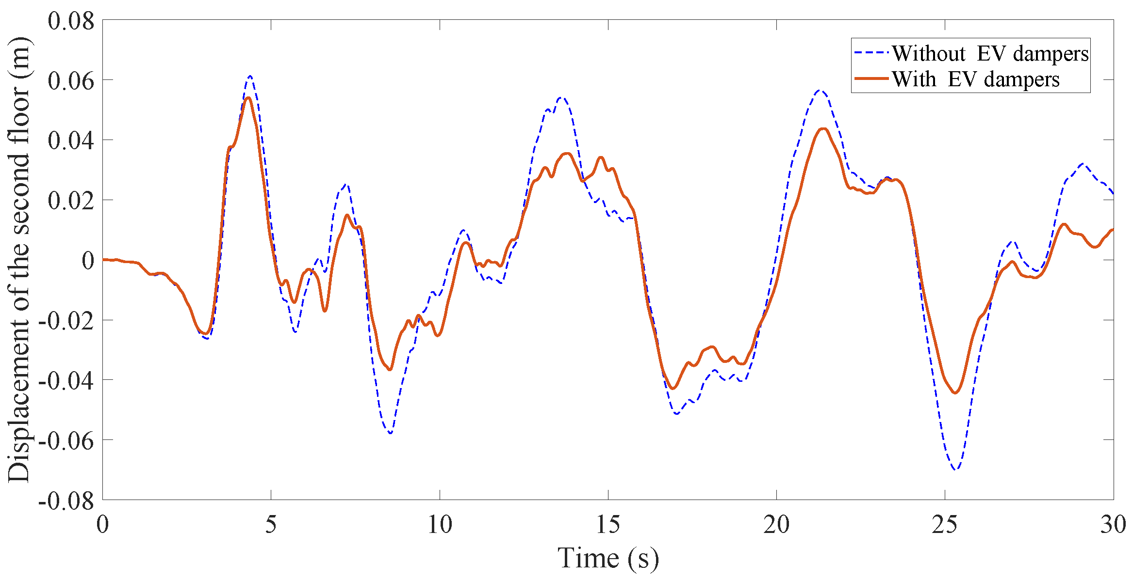
Second floor displacement of the building in the example in the El Centro earthquake.
Figure 24.
Second floor displacement of the building in the example in the El Centro earthquake.
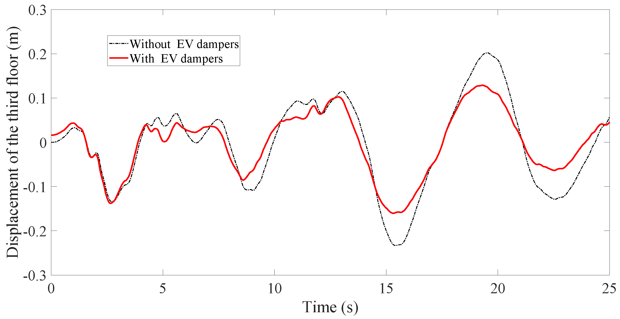
Figure 25.
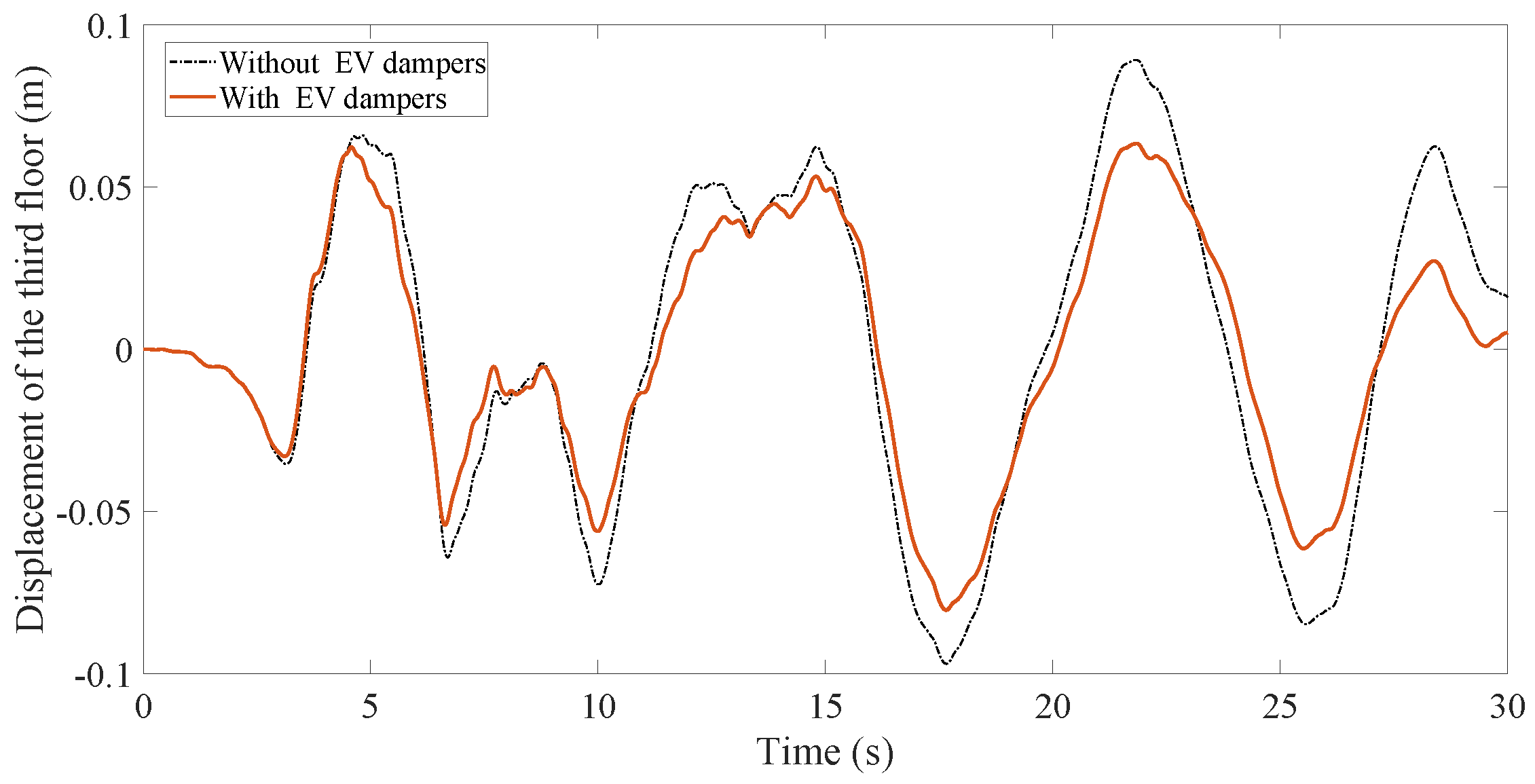
Third floor displacement of the building in the example in the El Centro earthquake.
Figure 25.
Third floor displacement of the building in the example in the El Centro earthquake.
Figure 26.
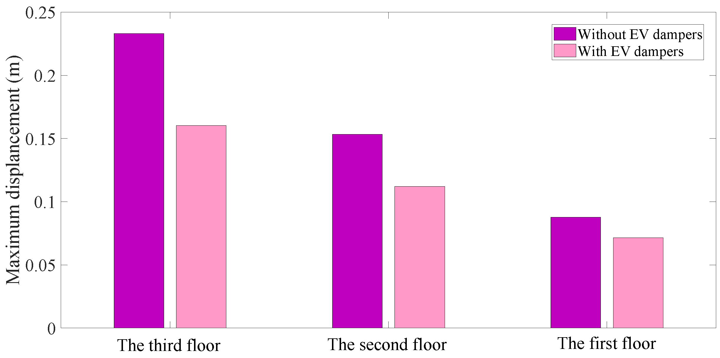
The maximum displacement of each floor in the El Centro earthquake.
Figure 26.
The maximum displacement of each floor in the El Centro earthquake.
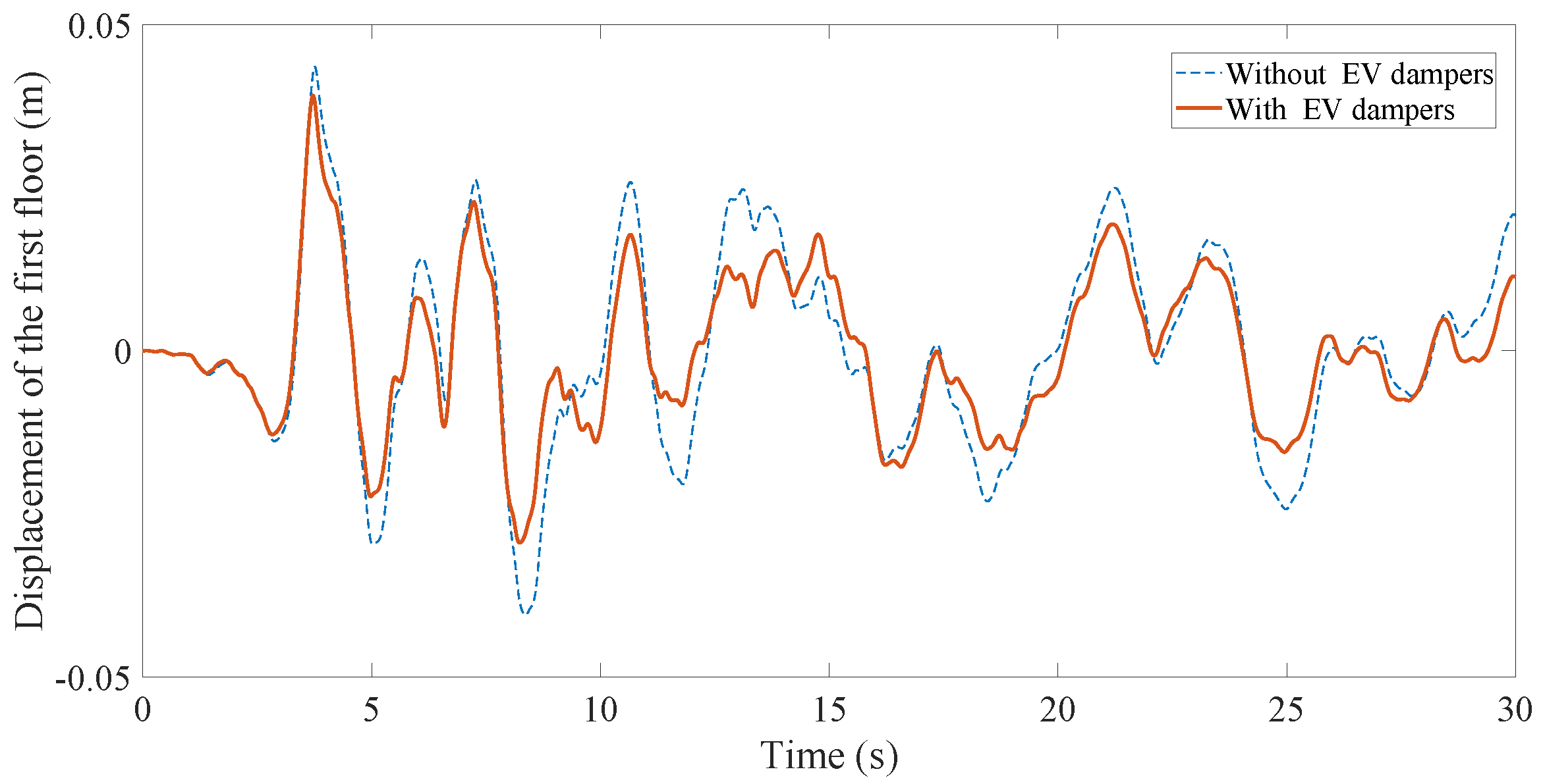
Figure 27.
First floor displacement of the building in the example in the Taft earthquake.
Figure 27.
First floor displacement of the building in the example in the Taft earthquake.
Figure 28.
Second floor displacement of the building in the example in the Taft earthquake.
Figure 28.
Second floor displacement of the building in the example in the Taft earthquake.
Figure 29.
Third floor displacement of the building in the example in the Taft earthquake.
Figure 29.
Third floor displacement of the building in the example in the Taft earthquake.
Figure 30.
The maximum displacement of each floor in the Taft earthquake.
Figure 30.
The maximum displacement of each floor in the Taft earthquake.
Table 1.
Parameters of the CFOPSO algorithm.
Table 1.
Parameters of the CFOPSO algorithm.
| CFOPSO Parameter | Value |
|---|
| Number of particles | |
| Number of iterations/Repeated experiments | |
| Scaling factors | |
| Chaotic bifurcation parameter | |
Table 2.
Parameters of the AEF-Zener model ( rad/s).
Table 2.
Parameters of the AEF-Zener model ( rad/s).
| Parameters | | | | |
|---|
| Values | | 0.651 | 3.849 | |
| Parameters | | | | |
| Values | | | −0.0013 | 0.0301 |
| Parameters | | | | |
| Values | 0.6526 | | | |
| Parameters | | | | |
| Values | | | | |
Table 3.
Parameters of the modified AEF-Zener model ().
Table 3.
Parameters of the modified AEF-Zener model ().
| Parameters | | | | |
|---|
| Values | | | | |
| Parameters | | | | |
| Values | | | | |
| Parameters | | | | |
| Values | | | | |
Table 4.
Comparison between experimental data and numerical results for the AEF-Zener model.
Table 4.
Comparison between experimental data and numerical results for the AEF-Zener model.
| | | Storage Modulus, | Loss Factor, |
|---|
| (rad/s) | () | Experimental | Numerical | Experimental | Numerical |
|---|
| 0.1 | −10 | 2.2740 | 2.2129 | 0.7765 | 0.6886 |
| −5 | 1.6951 | 1.7699 | 0.4904 | 0.5591 |
| 0 | 1.5043 | 1.3159 | 0.4012 | 0.4321 |
| 5 | 1.1530 | 1.0412 | 0.3170 | 0.3498 |
| 10 | 1.0232 | 0.9092 | 0.2681 | 0.2985 |
| 20 | 1.0037 | 0.9068 | 0.2413 | 0.2447 |
| 30 | 0.8111 | 0.7819 | 0.2201 | 0.2306 |
| 40 | 0.7360 | 0.7014 | 0.1940 | 0.2157 |
| 0.2 | −10 | 2.8233 | 2.7623 | 0.9332 | 0.9156 |
| −5 | 1.9408 | 2.1160 | 0.6119 | 0.6533 |
| 0 | 1.7612 | 1.5584 | 0.5132 | 0.4863 |
| 5 | 1.2341 | 1.2118 | 0.3573 | 0.3831 |
| 10 | 1.1123 | 1.0350 | 0.2905 | 0.3190 |
| 20 | 1.0481 | 0.9313 | 0.2612 | 0.2566 |
| 30 | 0.9068 | 0.8531 | 0.2380 | 0.2412 |
| 40 | 0.8034 | 0.7221 | 0.2121 | 0.2245 |
| 0.5 | −10 | 3.8227 | 3.7887 | 1.1168 | 1.1153 |
| −5 | 2.5560 | 2.7139 | 0.7635 | 0.8305 |
| 0 | 2.1240 | 1.9211 | 0.6923 | 0.6135 |
| 5 | 1.3250 | 1.4382 | 0.4423 | 0.4618 |
| 10 | 1.1710 | 1.1824 | 0.3353 | 0.3641 |
| 20 | 1.1262 | 1.0158 | 0.2940 | 0.2817 |
| 30 | 1.0231 | 0.9062 | 0.2693 | 0.2640 |
| 40 | 0.9114 | 0.8565 | 0.2433 | 0.2429 |
| 1.0 | −10 | 4.7551 | 4.4795 | 1.2049 | 1.2601 |
| 5 | 3.0626 | 3.2987 | 0.9186 | 0.9722 |
| 0 | 2.6408 | 2.5450 | 0.8185 | 0.8356 |
| 5 | 1.4614 | 1.3090 | 0.5468 | 0.5912 |
| 10 | 1.2840 | 1.1941 | 0.3848 | 0.4322 |
| 20 | 1.1967 | 1.0929 | 0.3274 | 0.3176 |
| 30 | 1.0897 | 1.0123 | 0.2920 | 0.2968 |
| 40 | 0.9786 | 1.0116 | 0.2605 | 0.2690 |
Table 5.
Root-mean-square error of and .
Table 5.
Root-mean-square error of and .
| | Storage Modulus, | Loss Factor, |
|---|
| Frequency (rad/s) | Root-Mean-Square Error (%) | Root-Mean-Square Error (%) |
|---|
| 0.1 | 9.65 | 4.47 |
| 0.2 | 11.16 | 2.23 |
| 0.5 | 11.63 | 3.89 |
| 1.0 | 15.41 | 3.64 |
Table 6.
The experimental and numerical results comparison of for different frequencies when mm and rad/s.
Table 6.
The experimental and numerical results comparison of for different frequencies when mm and rad/s.
| | Storage Modulus, (MPa) | Error |
|---|
| T ()
| Experimental | AEF Model | EFMCS Model | AEF Model | EFMCS Model |
|---|
| −10 | 4.7551 | 4.4795 | 4.4803 | 5.80% | 5.78% |
| −5 | 3.0626 | 3.2987 | 3.2900 | 7.71% | 7.41% |
| 0 | 2.6408 | 2.5450 | 2.5777 | 3.63% | 2.39% |
| 5 | 1.4614 | 1.3090 | 1.7995 | 9.28% | 23.14% |
| 10 | 1.2840 | 1.1941 | 1.5653 | 7.00% | 21.73% |
| 20 | 1.1967 | 1.0929 | 1.3847 | 8.67% | 15.71% |
| 30 | 1.0897 | 1.0123 | 1.1218 | 7.10% | 2.95% |
| 40 | 0.9786 | 1.0116 | 0.9389 | 3.37% | 4.06% |
Table 7.
The experimental and numerical results comparison of for different frequencies when mm and rad/s.
Table 7.
The experimental and numerical results comparison of for different frequencies when mm and rad/s.
| | Loss Factor, | Error |
|---|
| T (
) | Experimental | AEF Model | EFMCS Model | AEF Model | EFMCS Model |
|---|
| −10 | 1.2049 | 1.2601 | 1.3549 | 4.58% | 7.52% |
| −5 | 0.9186 | 0.9722 | 1.0225 | 5.83% | 11.31% |
| 0 | 0.8185 | 0.8356 | 0.7666 | 2.09% | 6.34% |
| 5 | 0.5468 | 0.5912 | 0.4608 | 8.12% | 15.73% |
| 10 | 0.3848 | 0.4322 | 0.3784 | 12.32% | 1.66% |
| 20 | 0.3274 | 0.3176 | 0.3234 | 3.00% | 1.22% |
| 30 | 0.2920 | 0.2968 | 0.2597 | 1.64% | 11.06% |
| 40 | 0.2605 | 0.2690 | 0.2253 | 3.26% | 13.51% |
Table 8.
The experimental and numerical results comparison of for different frequencies when mm and .
Table 8.
The experimental and numerical results comparison of for different frequencies when mm and .
| | Storage Modulus, (MPa) | Error |
|---|
| (rad/s) | Experimental | AEF Model | Xu’s Model | AEF Model | Xu’s Model |
|---|
| 0.1 | 1.0037 | 0.9068 | 0.9128 | 9.65% | 9.05% |
| 0.2 | 1.0481 | 0.9313 | 1.0119 | 11.14% | 3.45% |
| 0.5 | 1.1262 | 1.0158 | 1.1784 | 9.80% | 4.63% |
| 1.0 | 1.1967 | 1.0929 | 1.3379 | 8.67% | 11.80% |
Table 9.
The experimental and numerical results comparison of for different frequencies when mm and .
Table 9.
The experimental and numerical results comparison of for different frequencies when mm and .
| | Loss Factor, | Error |
|---|
| (rad/s) | Experimental | AEF Model | Xu’s Model | AEF Model | Xu’s Model |
| 0.1 | 0.2413 | 0.2447 | 0.2390 | 1.41% | 0.95% |
| 0.2 | 0.2612 | 0.2566 | 0.2646 | 1.76% | 1.30% |
| 0.5 | 0.2940 | 0.2817 | 0.2977 | 4.18% | 4.28% |
| 1.0 | 0.3274 | 0.3176 | 0.2917 | 2.99% | 9.07% |
Table 10.
Building parameters for the example.
Table 10.
Building parameters for the example.
| Floor | 1 | 2 | 3 |
|---|
| Quality (kg) | 2.40 × | 1.20 × | 1.20 × |
| Rigidity (N/m) | 1.08 × | 3.60 × | 2.16 × |


