Article

A New Approach to Determining the Network Fractality with Application to Robot-Laser-Hardened Surfaces of Materials

1
Complex Systems and Data Science Laboratory, Faculty of Information Studies, 8000 Novo Mesto, Slovenia
2
Department of Structural Mechanics and Analysis, Faculty of Mechanical Engineering and Transport Systems, Technical University Berlin, 10623 Berlin, Germany
*
Author to whom correspondence should be addressed.
Fractal Fract. 2023, 7(10), 710; https://doi.org/10.3390/fractalfract7100710
Submission received: 9 May 2023 / Revised: 20 September 2023 / Accepted: 22 September 2023 / Published: 27 September 2023

Abstract

:
A new method to determine a fractal network in chaotic systems is presented together with its application to the microstructure recognition of robot-laser-hardened (RLH) steels under various angles of a laser beam. The method is based on fractal geometry. An experimental investigation was conducted by investigating the effect of several process parameters on the final microstructures of material that has been heat-treated. The influences of the surface temperature, laser speed, and different orientation angles of the laser beam on the microstructural geometry of the treated surfaces were considered. The fractal network of the microstructures of robot-laser-hardened specimens was used to describe how the geometry was changed during the heat treatment of materials. In order to predict the fractal network of robot-laser-hardened specimens, we used a method based on intelligent systems, namely genetic programming (GP) and a convolutional neural network (CNN). The proposed GP model achieved a prediction accuracy of 98.4%, while the proposed CNN model reached 96.5%. The performed analyses demonstrate that the angles of the robot laser cell have a noticeable effect on the final microstructures. The specimen laser-hardened under the conditions of 4 mm/s, 1000 °C, and an impact angle of the laser beam equal to 75° presented the maximum fractal network. The minimum fractal network was observed for the specimen before the robot-laser-hardening process.

1. Introduction

The term “fractal” was proposed for the first time by Mandelbrot [1], derived from the Latin root “fract” (lat. “Fractare”—break, fraction; “fractus”—dismembered, broken; English “fractal”—fractional). According to Mandelbrot’s definition, a set is denoted as ‘fractal’ if its Hausdorff–Besikovich dimension is strictly greater than its topological dimension. Simply put, a fractal set is a set of dimensions different from what is usually called a topological dimension, represented by a number as a whole. Mandelbrot [1] also provided another definition: “a fractal is a structure made up of parts that resemble a whole in some way”. However, there is no strict and specific definition of a fractal today. A fractal structure is created by any infinitely repeating (iterating) initial shape, say H, in decreasing (or increasing) proportions, in a specific algorithm. This relatively simple feedback process provides a surprisingly diverse morphogenesis that often resembles the emergence of natural forms. Fractals are therefore characterized by self-similarity or large-scale invariance. Traditional geometric objects have integer dimensions: lines are one-dimensional, planes are two-dimensional, and spheres are three-dimensional. A fractal object is characterized by a fractal dimension. Such dimensions were introduced by F. Hausdorff. If a smooth Euclidean line just fills one-dimensional space, then the fractal line goes beyond it and partially fills two-dimensional space—its dimension is broken, and it lies between the original dimension of the line and the two-dimensional space of the fractal form Happened yes. The motivation of our research is presenting a new method for determining network fractality.
For example, fractal coastlines have dimensions between 1 and 2; fractal surfaces (mountains, clouds) have dimensions between 2 and 3. The fractal dimension [2] is a topological invariant of every fractal structure, which is a special symmetry. So, as mentioned earlier, fractal lines go beyond one-dimensional space into two-dimensional space. Their dimensions are broken, and lie between the original dimension of lines and the two-dimensional space of morphogenesis—fractal genesis. Likewise, fractal planes extend partially into three-dimensional space; theoretically, we also believe that the output of a three-dimensional surface is the result of its fractalization into higher-dimensional spaces. For example, coastlines and many other natural structures and processes are fractal (or, more accurately, quasi-fractal): rivers and their tributaries, lightning, mountain surfaces, cloud cover, the distribution of galaxies, solar activity. The natural landscape around us is created by the dynamic chaos of natural processes. The fractal properties of natural objects demonstrate the ability to construct very realistic computer landscapes, virtual worlds, in relatively simple fractal programs, where the resemblance to reality is achieved through randomization and a certain degree of irregularity achieved through random number management. However, fractals can also be indistinguishable, such as scaly, granular, fibrous fractals, etc. The self-similarity of fractal structures as a result of functional iteration with reverse communication (self-referential feedback) determines near (local) connections to distant (global) orders and enables concise mathematical descriptions of structures and processes. These structures and processes are hardly suitable for mathematical description and mathematical understanding. Simple mathematical rules generate self-similar structures with respect to nonlinear transformations, thus enabling fairly complex shapes. This means that simple laws are at the very heart of complex systems and processes. The application of fractal structures in the field of mechanical engineering is most developed in fractal systems. Brittle iron is relatively weak, Mandelbrot also said. Fractal geometry has been successfully used for the detailed analysis of various mechanical properties of materials such as molybdenum, stone, concrete, steel, and composite materials of various lengths. The values obtained from the analyzed fracture sites confirm the concept of a global fracture measurement, independent of the fracture analysis obtained by scientific researchers for this type of material. This approach also facilitates product integration.
Robot laser hardening (RLH) belongs to the group of modern and highly effective methods for hardening the surface layers of materials [3]. Thermal hardening of metals and alloys occurs locally when a portion of the radiation surface is heated followed by the fast cooling of this surface portion due to the removal of heat to the internal cold metal layers. Important advantages of laser hardening also include the reduction in the additional processing of the material, the eliminated need for a separate cooling process, and the ability to process inhomogeneous 3D blanks and complex geometries. Robot systems that provide not only heat treatment, but also positioning, the automatic feeding of workpieces, results measurement, etc., are becoming more relevant. The complex control system analyzes this data stream in real-time and, if necessary, corrects the parameters of laser radiation. This is important in the conditions of practical work when the workpiece warms up in the process of heat hardening. If the radiation power is not proportionally adjusted, overheating will occur, causing deterioration in the results of the heat-hardening process. The control system provides automatic calibration in the framework of the service tasks and makes appropriate corrections in the technological operations performed.
Heat-treatment processes, including the hardening and tempering of tool steels to achieve a desired microstructure with improved mechanical properties, is one of the last production steps which determines the final bulk residual stresses within the workpiece [4]. Babič et al. [5] presented a procedure based on the calculation of the FD complexity index. It was developed to assess the complex geometry of RLH materials’ microstructures upon changing the process parameters, and the obtained results were in agreement with experimental data.
Modeling of thermo-mechanical–metallurgical interactions during heat treatment is quite important in order to predict the evolution of internal stresses and distortions as a consequence of the process [6].
Babič et al. [
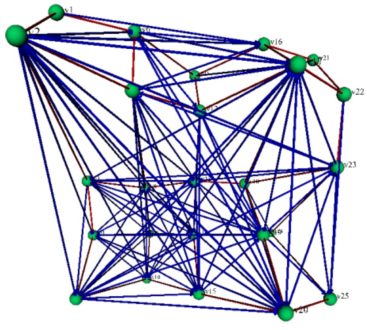
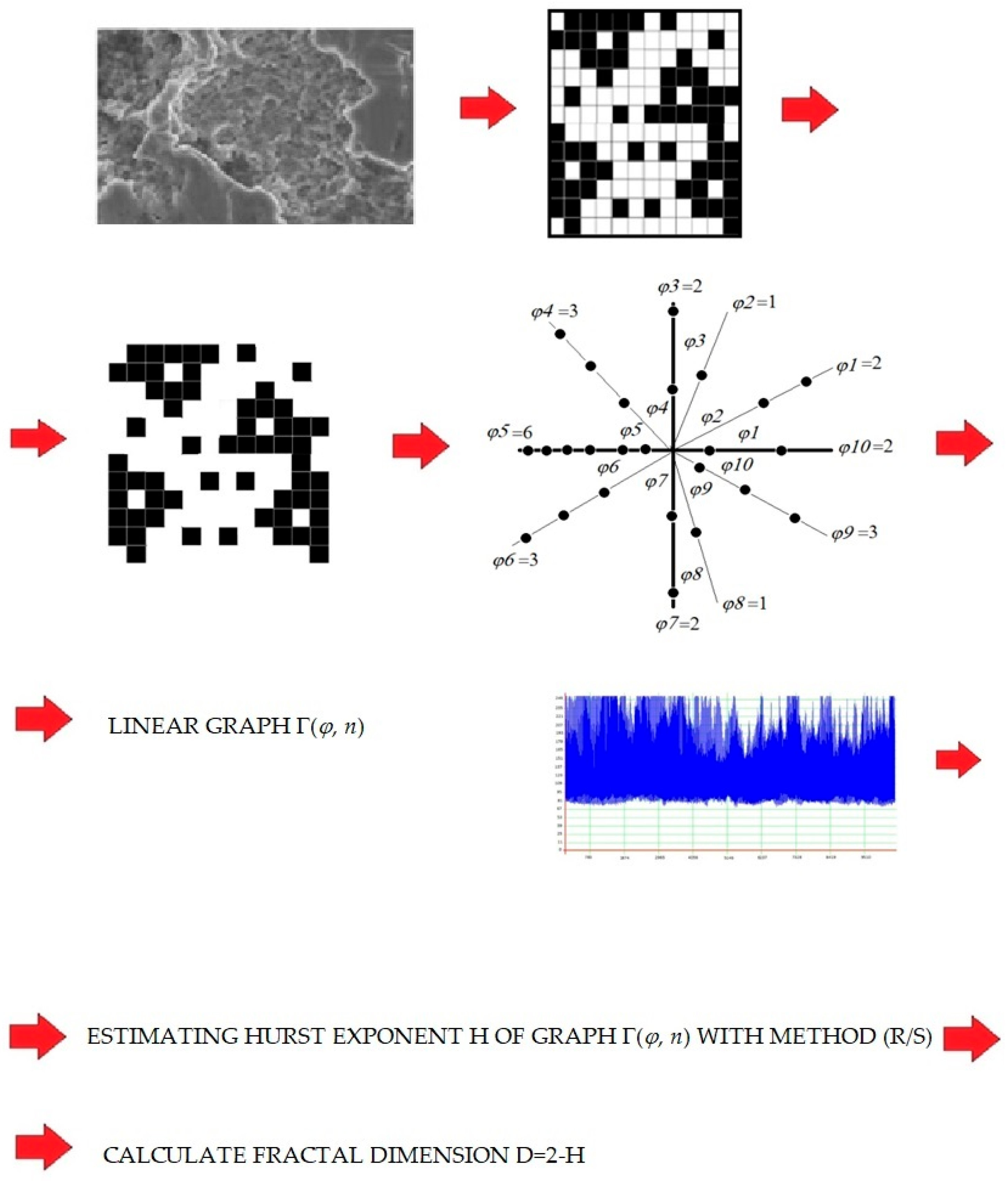
7] introduced a new method for quantifying the complexity of networks based on the network nodes given in Cartesian coordinates. The nodes were mapped to polar coordinates, and fractal dimensions were computed using the ReScaled Ranged (R/S) method. This work revealed various challenges, thus calling for further research in this field.
The aim of this manuscript is to propose a new approach to determining network fractality, with an application to robot-laser-hardened surfaces of materials, and to modeling the fractal networks of RLH specimens’ microstructures depending on the process parameters of the robot laser cell.
Section 2 presents the preparation of materials, methodology and data mining, and Section 3 gives the results and discussion, while conclusions are given in the last section.

2. Material Preparation, Methodology and Data Mining

2.1. Material Preparation

In the present study, steel standard tools [8] were hardened using a laser cell, equipped with a robot RV60-40 by Reis Robotics Company from Obernburg, Germany (technical details: manufacturer: Reis Robotics; model: HRV60; category: industrial robots; weight: 1200 kg; height: 100 com; length: 200 cm; width: 100 cm). The robot controls the laser head position and the laser beam orientation (fiber coupled 10 kW diode, laser Laserline LDF10000, 1.5 µm fiber). The laser can deliver a nominal maximum power equal to 1500 W. The manufacturing cell is also equipped with a thermal scanner that measures the surface temperature during the heat treatments.
During the experiments, the following process parameters were controlled:
Laser beam speed v ∈ [2 mm/s, 5 mm/s];
Surface temperature T ∈ [850 °C, 1400 °C];
Impact angles φ ∈ [45°, 60°, 75°], φ ∈ [105°, 120°, 135°].
Figure 1 provides schematic views of the laser hardening performed by the robot, including different options to modify the laser beam angle, either in the plane defined by the laser motion or in the plane perpendicular to it. Each robot-laser-hardened specimen was etched (selective removal of material from a sample using chemical or physical means) and polished (an abrasive material was used to finish the metal surface), which was carried out at the Institute of Metals and Technology (IMT) in Ljubljana, Slovenia. Afterwards the samples were studied under a microscope at the Jožef Stefan Institute IJS in Ljubljana, Slovenia. The image in Figure 2 was obtained by field emission scanning electron microscopy using a JMS-7600F from JEOL (Tokyo, Japan) and represents the complexity of the microstructure.
Figure 2 depicts the microstructure of a laser-hardened specimen, with hardening performed by a robot. The magnification used for SEM is 2000×, and the image resolution is 250 × 200 pixels.

2.2. Methodology

First, we apply a network of interconnected nodes [9] to describe the microstructure. A node is one of the two most distinctive elements of such a diagram, often understood as an apex. It represents an intersection. This could be a particular position, property, etc. It is typically envisaged as a sphere. Another most cardinal characteristic of the diagram is the links. A link is an association between two nodes. Typically, it is shown as a line connecting two nodes. Figure 3 illustrates such a network.
Furthermore, we apply fractal geometry to describe the complexity of the investigated geometry. Dimensions of self-similar fractals are the same at each enlargement, which is not an issue for statistical unmixed-relative fractals [10]. Figure 4 depicts self-similar and self-affine transformations. Self-affine transformations are also tilting transformations.
It may be emphasized that the self-similarity space is a subset of self-affinity. Self-affine fractals—including self-similar geometry—can be divided into exactly self-affine, quasi-self-affine and statistically self-affine, as shown in Figure 5.
The two-dimensional representation of the RLH specimen’s microstructure is quite complicated and definitely not perfectly alike but can still be examined statistically using the mentioned approach. Canonical Euclidean geometry cannot be applied to this problem. Thus, fractal geometry was selected for this purpose. We developed a new method to estimate fractal properties of the network, and it is presented below.
First, we convert SEM images into binary images (black and white squares). Then, we use only black squares, i.e., we remove the white ones. The black squares present the nodes of the network. We convert all these black nodes into a polar coordinate system with coordinates (r, φr). For each line φi, we check how many of the nodes lie on it (n). So, φi = n. We determine all pairs (φi, n), which results in a linear graph Γ(φ, n). In addition, the linear graph Γ(φ, n) includes nodes T1(φ1, n1), T2(φ2, n2) … Tk(φk, nk). For this graph, we estimate the Hurst exponent H [11]. After this, we can calculate the fractal dimension using the equation D = 2 − H. The Hurst exponent has a value in the interval H ∈ (0, 1); thus, the fractal dimension of complex networks is D ∈ (1, 2). Figure 6 shows the procedure of calculating the fractal dimension of the network.

2.3. Data Mining

We use methods of intelligent systems [12] to predict the complexity of the microstructures of robot-laser-hardened specimens—we use CNN, GP and MR.
Genetic programming (GP) [11,13] is an approach based on the creative power inherent in natural evolution for the automatic development of computer programs. It tries to imitate mechanisms of natural evolution in order to automatically generate programs that solve a given problem. GP has been used successfully in a number of applications for both solving purely mathematical problems and solving real-world problems. We used the following attributes of the GP: size of the population of organisms: 600; maximum number of generations: 100; reproduction probability: 0.5; crossover probability: 0.6; maximum permissible depth in the creation of the population: 8; maximum permissible depth after the operation of the crossover of two organisms: 10; smallest permissible depth of organisms in generating new organisms: 4; and tournament size used for the selection of organisms: 7. Parameters are given in Table 1.
Deep learning neural networks have a particular subset known as convolutional neural networks, sometimes known as CNNs or ConvNets [14]. The inputs to a CNN are often pictures, and it uses one or more convolutional layers that typically conduct a 2D convolution. CNNs have gained a lot of popularity recently and have produced some truly remarkable image recognition results that have had a significant impact on the field of computer vision. John von Neumann first suggested the concept of cellular automata (CAs) [15]. Although it is evident that the speed and temperature of the robot laser have a significant impact on the fractal dimension of the network of the microstructure of RLH specimens, we were curious as to whether this prediction could be strengthened by looking at specimen photos. Our objective was to determine whether the fractal dimension of the network of the microstructure of RLH specimens can be predicted from the specimen photos, and if so, whether this prediction is much more accurate than the one that relies just on the speed and temperature. We applied two settings:
  • To forecast the fractal dimension of the network of the microstructure of RLH specimens without photos, only non-image input parameters were used.
  • In addition to other input characteristics, images were also employed to forecast the fractality of the network of the microstructure of RLH specimens.
In the first instance, the network fractality of RLH specimens’ microstructures was predicted using two inputs—temperature and speed—based on a standard multilayer perceptron. In the second instance, as seen in Figure 7, a convolutional neural network (CNN) was used to forecast the network fractality of the microstructure of RLH specimens.

3. Results, Discussion, GP and CNN Approach

In 
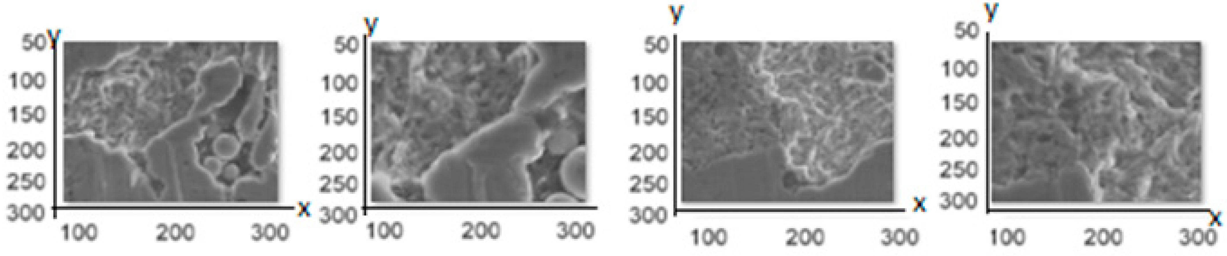
Table 2, the parameters and the network fractality of RLH specimens are presented. We mark specimens from S1 to S22. The parameter X1 represents the temperature [°C], X2 is the speed of hardening (mm/s), X3 is the angle (°) of hardening, X4 is the number of nodes of the fractal network and Y represents the network fractality of the RLH specimens. S1–S4 are the specimens hardened using the process presented in Figure 1. Specimens S5–S8 represent the material next to the hardened zone. S9–S11 represent the results of the robot laser hardening under the following conditions: the variation in the angle φ ∈ (45, 60, 75)° between the left side of the laser beam and the material surface. S12–S14 represent the results of the robot laser hardening under these conditions: the variation in the incidence angle φ ∈ (45, 60, 75)° between the right side of the laser beam and the material surface. S15–S17 represent the results of the robot laser hardening under another set of conditions: the angle was changed in the plane defined by the direction of the laser beam φ ∈ [45°, 60°, 75°]. S18–S20 represent the results of robot laser hardening under the final set of variable conditions: the angle was changed in the plane perpendicular to the direction of the laser beam φ ∈ [105°, 120°, 135°]. S21 represents the results of the point-robot-laser-hardened specimens. Finally, specimen S22 represents the material before using the process of hardening. 
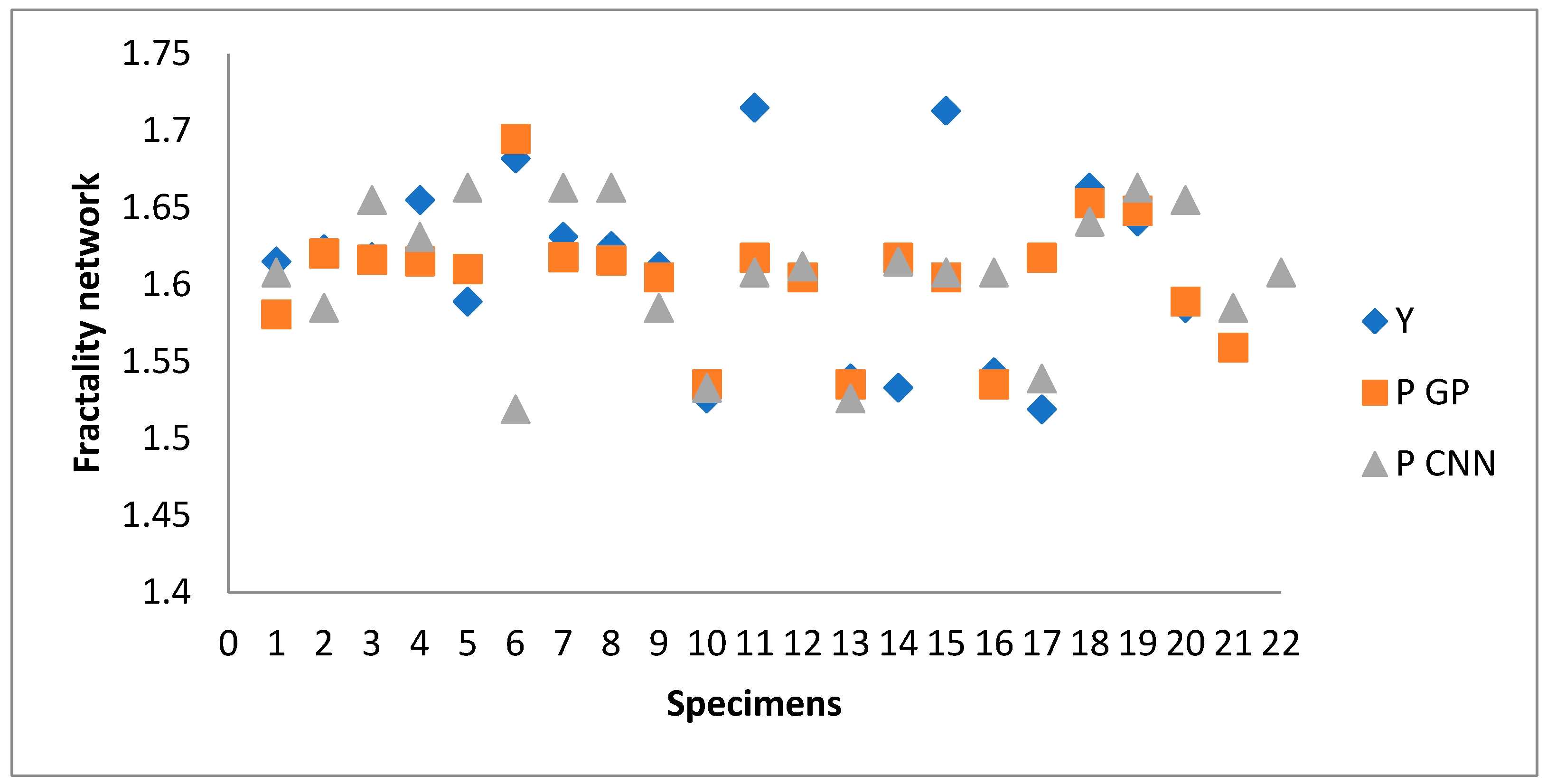
Table 3 gives the measured and predicted network fractality of RLH specimens, while Figure 8 gives the predicted network fractality of RLH specimens by using GP and CNN.
The laser heat treatment technique for robots is straightforward, but this study reveals that the evolution of the microstructure during the laser-hardening process is an important aspect that needs to be addressed. It shows that the changing laser beam angles affect the intricate networks that make up the microstructure of specimens that were laser-hardened by means of robots. The proposed technique allows identifying the complicated network structure discovered in the microstructure of laser-hardened specimens at various angles. The maximum complexity specification is obtained for specimen S11: 1.715. This specimen was hardened at a rate of 4 mm/s at 1000 °C with the variation in the incidence angle φ ∈ 75° between the left side of the laser beam and the material surface. The minimal complexity was observed for the specimen S22, which represents the material before the robot-laser-hardening process. Hence, the complexity of the microstructure of the robot-laser-hardened specimens indicates how the heat treatment of a material alters its microstructure’s geometry.
Furthermore, the network complexity of microstructural materials hardened at various speeds, temperatures, and laser beam angles is modeled using genetic programming (GP). The measured data and the genetic programming model data yield a high agreement of 98.4%. As a result, the complexity network parameter X3 (angle) has a greater effect on the model. In order to create 100 different predictions based on the various parameters employed in the robot laser cell, the internal GP system was executed 100 times. On an I7 Intel processor (Intel Corporation, Santa Clara, CA, USA) with 8 GB of RAM, each run lasted roughly 2.5 h. Using an internal genetic programming system written in AutoLISP and connected with AutoCAD (v24.2), we used 100 separate models for forecasting network fractality of RLH specimens. The mean square of errors from the monitored data was used to measure the model’s fitness. It is given by
Δ = ΣΔi2/n,
where i is the square of the error of a single sample of data, and n is the size of the monitored data.
Simply put, an individual organism’s single sample data variance is
Δi = Ei − Gi
where Ei and Gi are the projected and actual scrap fractions, respectively, and they only depend on the surface flaws.
The developed optimal model of genetic programming is given as follows:
Y = 1.83992 0.118464   ×   ( 1.83992 + ( 8.50567   ×   ( 0.454976 × X 1 X 3 X 1 ( 2.19792 + 0.312703 × X 1 X 3 ) + 2 × X 2 + 2.19792 + X 3 5.28948 × ( 2.19792 X 1 X 4 ) 4.39584 1 X 2 X 2 0.059118 × X 3 + X 1 X 2 ( X 1 X 3 + X 3 ) 2.19792 + X 3 5.28948 × ( 0.454976 × X 1 X 3 X 3 X 4 ) 4.39584 1 X 2 X 2 0.059118 × X 3 + X 1 X 2 ( X 1 X 3 + X 3 )   ) ) / ( X 3 2 X 2 2.19792 + X 3 0.189055 × ( X 3 2.19792 + X 3 0.189055 × X 3 X 4 2.19792 0.312703 × X 1 X 3   ) 2.19792 X 1 X 4 4.81742 1 + X 2 X 3 + X 1 X 2 ( X 3 + X 1 X 3 × X 3 ) ) )
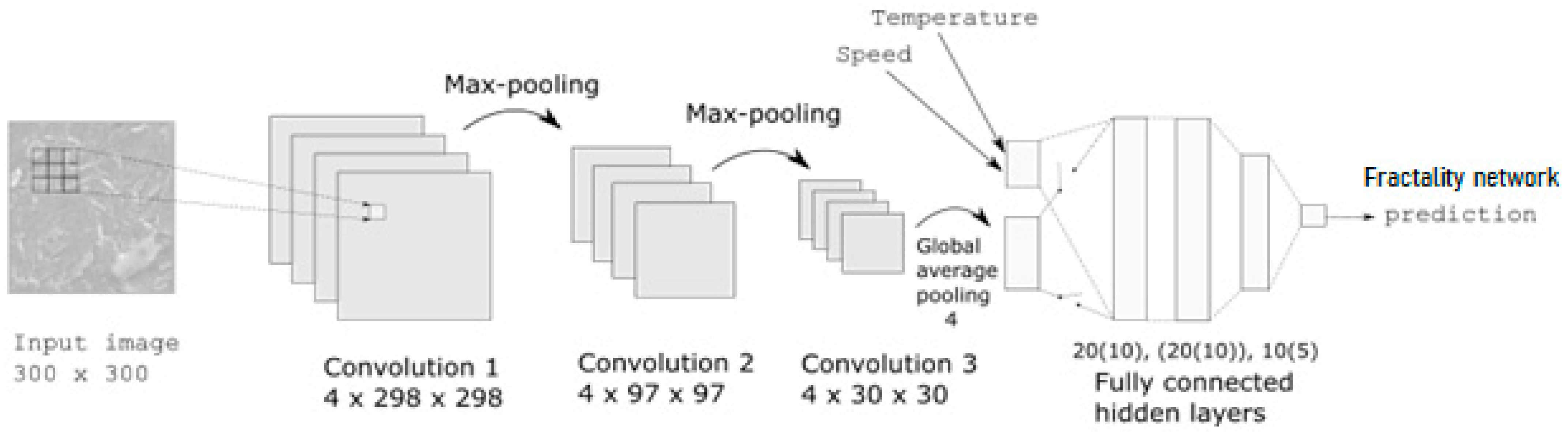
The specimen photos were reduced to a standard of 300 × 300 pixels. There was just one channel needed because they were given as grayscale. The values were scaled from the [0, 255] interval to the [0, 1] interval. To reduce the image size further, a two-dimensional max-pooling (3 × 3) layer was applied after a two-dimensional convolution layer with a filter size of 3 × 3 and four kernels. The 2D conv-layer and max-poling combination were used once more to obtain more compression. The third convolutional layer and an average pooling layer, whose output was flattened so that it could be combined with the non-image data, were then applied. Figure 9 presents the microstructure of one example of 22 specimens characterized by speed treatments of 2 mm/s (S1), 3 mm/s (S2), 4 mm/s (S3), and 5 mm/s (S4) at 1000 °C.
The RMSprop learning method was used to train the CNNs over 1200 iterations at a learning rate of 0.001 error in the mean square (MSE). Both examined cases, those without photographs and those with images, had their mean squared error (MSE) recorded. Eight training configurations were tested for each setting, including two and three hidden layers, two different layer sizes (i.e., the number of artificial neurons), and two different activation modes for the neurons (sigmoid vs. relu). The output neuron’s activation function was always sigmoid, and it was utilized to predict the surface roughness. Table 4 represents the findings. The average of 10 runs, along with the standard deviation, is the outcome for each round of training. For each parameter set (speed, temperature), two of the three photos were utilized for training, and the third one was used for testing. Therefore, we also have test results in the “image” setting. Because testing would produce identical results for the training in the “no-image” mode, only the training’s findings are provided. The bold numbers in Table 4 are the best results obtained by means of CNN. The CNN model delivers a precision of 96.5%.

4. Conclusions

With the aim of analyzing the invariance property of the network fractality of real microstructure images (and fractography), it was necessary to develop a new method for determining the object complexity that can be seen in the microstructures of RLH specimens. In order to predict the complexity of robot-laser-hardened specimens, we applied an AI method, namely genetic programming. The genetic programming delivered an accuracy of above 98%.
The highest complexity specification was found for the specimen S11: 1.715. This specimen was hardened at a rate of 4 mm/s, at 1000 °C, with the variation in the incidence angle of φ ∈ 75° between the left side of the laser beam and the material surface. The minimal network fractality was found in the specimen before the RLH process. Finally, because the microstructure of RLH specimens is very chaotic and complex, it is clear that for the use of fractal-based analysis for the evaluation of the microstructure of RLH materials, careful calibrations are required to develop a technological tool for real-life application. There are a number of aspects that remain to be investigated to obtain a complete understanding of the fractal behavior of microstructures of RLH specimens using images and in order to implement its application for the evaluation of materials.
Furthermore, we successfully applied a convolutional neural network (CNN) to predict the surface roughness also using the photos of the materials’ surfaces. The mean squared error was in the range from 0.021 ± 0.002 to 0.015 ± 0.001 when images were also used. A t-test was applied to compare the means, yielding t = 0.023/0.017 = 1.35 at 16 degrees of freedom. This implies that the p-value is equal to 0.18. Hence, the prediction using images noticeably improved compared to the case when images were not used. The CNN model delivered a precision of 96.5%.
Making sprockets extremely hard throughout the hardening process is a very significant issue. In this study, we described a novel technique for hardening materials under various laser beam angles using a robot laser cell to address the issue of sprocket hardening (the idea of two laser-beam RLH). We split the laser beam into two parts using a prism. In the future, we intend to investigate the effects of different laser beam angles and characteristics on the topography of various materials using two laser beams for RLH.
An important advantage of the proposed method is its applicability in a wide range of fields such as in medicine, in the analysis of biochemical interactions, in the analysis of biomedical images in technical science, in the analysis of the influence of process parameters on a material’s mechanical properties, and even in social sciences. Of course, until more knowledge is acquired about its application in various fields, the method is to be used with special care.

Author Contributions

Conceptualization, M.B. and D.M.; methodology, M.B.; software, M.B.; validation, M.B. and D.M.; formal analysis, M.B. and D.M.; investigation, M.B. and D.M.; resources, M.B. and D.M.; data curation, M.B. and D.M.; writing—original draft preparation, M.B. and D.M.; writing—review and editing, M.B. and D.M.; visualization, M.B. and D.M.; supervision, M.B. and D.M.; project administration, M.B. and D.M.; funding acquisition, M.B. and D.M. All authors have read and agreed to the published version of the manuscript.

Funding

We acknowledge support by the German Research Foundation and the Open Access Publication Fund of TU Berlin.

Data Availability Statement

Not applicable.

Acknowledgments

We acknowledge support by the German Research Foundation and the Open Access Publication Fund of TU Berlin.

Conflicts of Interest

The authors declare no conflict of interest.

References

  1. Mandelbrot, B.B. Fractal aspects of the iteration of z→λz(1−z) for complex λ and z. In Fractals and Chaos; Springer: New York, NY, USA, 2004. [Google Scholar] [CrossRef]
  2. Oborny, B. Scaling Laws in the Fine-Scale Structure of Range Margins. Mathematics 2018, 6, 315. [Google Scholar] [CrossRef]
  3. Frerichs, F.; Lu, Y.; Lübben, T.; Radel, T. Process Signature for Laser Hardening. Metals 2021, 11, 465. [Google Scholar] [CrossRef]
  4. Shugurov, A.R.; Nikonov, A.Y.; Dmitriev, A.I. The effect of electron-beam treatment on the deformation behavior of the EBAM Ti-6Al-4V under scratching. Facta Univ. Ser. Mech. Eng. 2022, 20, 307–319. [Google Scholar] [CrossRef]
  5. Babič, M.; Marinkovic, D.; Bonfanti, M.; Calì, M. Complexity Modeling of Steel-Laser-Hardened Surface Microstructures. Appl. Sci. 2022, 12, 2458. [Google Scholar] [CrossRef]
  6. Yaakoubi, M.; Kchaou, M.; Dammak, F. Simulation of the thermomechanical and metallurgical behavior of steels by using ABAQUS software. Comput. Mater. Sci. 2013, 68, 297–306. [Google Scholar] [CrossRef]
  7. Babič, M.; Marinković, D.; Kovačič, M.; Šter, B.; Calì, M. A New Method of Quantifying the Complexity of Fractal Networks. Fractal Fract. 2022, 6, 282. [Google Scholar] [CrossRef]
  8. DIN EN 10083-1; Steels for Quenching and Tempering—Part 1: General Technical Delivery Conditions. Deutsches Institut für Normung: Berlin, Germany, 2006.
  9. Bezerra Rodrigues, R.A.; Cicek, J.S.; Zacharias, K.; Paul, J. How Actor-Network Theory Travels and Changes in Engineering Education: A Narrative Literature Review. In Proceedings of the 2022 ASEE Annual Conference & Exposition, Minneapolis, MN, USA, 26–29 June 2022; Available online: https://peer.asee.org/41682 (accessed on 30 April 2023).
  10. Zhang, Q.; Pei, Y.; Shen, Y.; Wang, X.; Lai, J.; Wang, M. A New Perspective on Predicting Roughness of Discontinuity from Fractal Dimension D of Outcrops. Fractal Fract. 2023, 7, 496. [Google Scholar] [CrossRef]
  11. Kovačič, M.; Župerl, U. Genetic programming in the steelmaking industry. Genet. Program. Evolvable Mach. 2020, 21, 99–128. [Google Scholar] [CrossRef]
  12. Buiten, M.C. Towards Intelligent Regulation of Artificial Intelligence. Eur. J. Risk Regul. 2019, 10, 41–59. [Google Scholar] [CrossRef]
  13. Madić, M.; Gostimirović, M.; Rodić, D.; Radovanović, M.; Coteaţă, M. Mathematical modelling of the CO2 laser cutting process using genetic programming. Facta Univ. Ser. Mech. Eng. 2022, 20, 665–676. [Google Scholar] [CrossRef]
  14. Valueva, M.V.; Nagornov, N.N.; Lyakhov, P.A.; Valuev, G.V.; Chervyakov, N.I. Application of the residue number system to reduce hardware costs of the convolutional neural network implementation. Math. Comput. Simul. 2020, 177, 232–243. [Google Scholar] [CrossRef]
  15. Jingyi, X.; Li, Z. Application of Cellular Automata with Improved Dynamic Analysis in Evacuation Management of Sports Events. J. Sens. 2022, 2022, 8782865. [Google Scholar] [CrossRef]
Figure 1. Schematic view of the laser hardening via robot: (a) the laser beam impacts the treated surface perpendicularly (90°); (b) the impact angle modified to the right or left side: φ ∈ [45°, 60°, 75°] and [105°, 120°, 135°], respectively; (c) the impact angle modified forward: φ ∈ [45°, 60°, 75°]; (d) the impact angle is modified downward: φ ∈ [105°, 120°, 135°]; (e) robot laser hardening with overlapping; (f) point robot laser hardening (the laser beam does not move).
Fractalfract 07 00710 g001aFractalfract 07 00710 g001b
Figure 2. Microstructure of a laser-hardened specimen using a robot.
Fractalfract 07 00710 g002
Figure 3. Example of graph/network.
Fractalfract 07 00710 g003
Figure 4. Self-similar and self-affine transformations.
Fractalfract 07 00710 g004
Figure 5. Three types of self-similar fractal objects: (a) self-similar geometric object; (b) quasi-self-similar natural object; (c) statistically self-affine microstructure of robot-laser-hardened specimen.
Fractalfract 07 00710 g005
Figure 6. Procedure of calculating fractal dimension of the network.
Fractalfract 07 00710 g006
Figure 7. Convolutional neural network. In the first setting (without images), the global average pooling layer is not connected to fully connected layers, while in the second (with images), it is connected.
Fractalfract 07 00710 g007
Figure 8. The calculated and predicted network fractality of RLH specimens based on GP and CNN.
Fractalfract 07 00710 g008
Figure 9. Microstructure of specimens characterized by a speed treatment of (from left to right) 2 mm/s (S1), 3 mm/s (S2), 4 mm/s (S3), and 5 mm/s (S4) at 1000 °C.
Fractalfract 07 00710 g009
Table 1. Attributes of the GP.
Attributes#
size of the population of organisms600
maximum number of generations100
reproduction probability0.5
crossover probability0.6
maximum permissible depth in the creation of the population8
maximum permissible depth after the operation of crossover of two organisms10
smallest permissible depth of organisms in generating new organisms4
tournament size used for selection of organisms7
Table 2. Parameters of RLH specimens.
SX1X2X3X4Y
S11000290120,5151.615
S21000390125,5791.623
S31000490123,6951.618
S41000590124,5851.655
S51400290124,3781.589
S61400390132,2921.682
S71400490126,7141.631
S81400590130,7511.625
S91000245123,3451.612
S101000360126,1471.526
S111000475124,0481.715
S121000245123,5811.608
S131000360127,8951.539
S141000475122,1521.533
S151000245120,3701.713
S161000360116,5641.543
S171000475132,7831.519
S1814000105130,2261.663
S1910000120130,7951.641
S209500135106,4681.585
S21850090120,5651.559
S2200094,8421.374
Table 3. The measured and predicted network fractality of RLH specimens.
SYP GPP CNN
S11.6151.580721.608
S21.6231.620351.585
S31.6181.616311.655
S41.6551.615131.631
S51.5891.610241.663
S61.6821.694761.519
S71.6311.617951.663
S81.6251.615761.663
S91.6121.604831.585
S101.5261.535241.533
S111.7151.617461.608
S121.6081.604831.612
S131.5391.535241.526
S141.5331.617461.615
S151.7131.604831.608
S161.5431.535241.608
S171.5191.617461.539
S181.6631.652911.641
S191.6411.648081.663
S201.5851.589191.655
S211.5591.559131.585
S221.3741.373641.608
Table 4. Roughness prediction errors (the mean squared error, MSE) in both settings: without and with images.
Number of
Hidden Layers
Size of
Layers
Activation
Function
Without ImagesWith Images
Train (=Test)TrainTest
Mean StdMean StdMean Std
2 hidden layers20, 10sigmoid0.022 ± 0.0010.021 ± 0.0020.022 ± 0.002
relu0.024 ± 0.0020.018 ± 0.0030.017 ± 0.003
10, 5sigmoid0.027 ± 0.0010.028 ± 0.0040.028 ± 0.004
relu0.024 ± 0.0030.021 ± 0.0040.022 ± 0.004
3 hidden layers20, 20, 10sigmoid0.022 ± 0.0010.019 ± 0.0020.021 ± 0.002
relu0.021 ± 0.0020.015 ± 0.0010.015 ± 0.001
10, 10, 5sigmoid0.026 ± 0.0010.026 ± 0.0030.027 ± 0.002
relu0.025 ± 0.0040.021 ± 0.0050.021 ± 0.004
Disclaimer/Publisher’s Note: The statements, opinions and data contained in all publications are solely those of the individual author(s) and contributor(s) and not of MDPI and/or the editor(s). MDPI and/or the editor(s) disclaim responsibility for any injury to people or property resulting from any ideas, methods, instructions or products referred to in the content.

