Article

Metaheuristic Solution for Stability Analysis of Nonlinear Systems Using an Intelligent Algorithm with Potential Applications

1
Laboratory Modélisation, Analyse et Commande des Systèmes, University of Gabes, Gabes LR16ES22, Tunisia
2
Department of Industrial Engineering, College of Engineering, University of Ha’il, Hail 2440, Saudi Arabia
3
Department of Information and Computer Science, College of Computer Science and Engineering, University of Ha’il, Hail 2440, Saudi Arabia
4
School of Industrial Engineering, Pontificia Universidad Católica de Valparaíso, Valparaíso 2362807, Chile
5
Faculty of Automatic Control and Computer Science, University Politehnica of Bucharest, RO-060042 Bucharest, Romania
6
Department of Mechanical Engineering, College of Engineering, University of Ha’il, Hail 2440, Saudi Arabia
*
Authors to whom correspondence should be addressed.
Fractal Fract. 2023, 7(1), 78; https://doi.org/10.3390/fractalfract7010078
Submission received: 14 December 2022 / Revised: 31 December 2022 / Accepted: 5 January 2023 / Published: 10 January 2023

Abstract

:
In this article, we provide a metaheuristic-based solution for stability analysis of nonlinear systems. We identify the optimal level set in the state space of these systems by combining two optimization phases. This set is in a definite negative region of the time derivative for a polynomial Lyapunov function (LF). Then, we consider a global optimization problem stated in two phases. The first phase is an external optimization to search for a definite positive LF, whose derivative is definite negative under linear matrix inequalities. The candidate LF coefficients are adjusted using a Jaya metaheuristic optimization algorithm. The second phase is an internal optimization to ensure an accurate estimate of the attraction region for each candidate LF that is optimized externally. The key idea of the algorithm is based mainly on a Jaya optimization, which provides an efficient way to characterize accurately the volume and shape of the maximal attraction domains. We conduct numerical experiments to validate the proposed approach. Two potential real-world applications are proposed.

1. Introduction

A relevant problem in control engineering is examining the equilibrium point’s asymptotic stability in nonlinear dynamical processes. A nonlinear analysis regularly estimates the asymptotic stability domain for equilibrium points [1]. A domain of attraction (DA) is where the dynamical behavior of the system’s state variables is asymptotically stable. As the initial states converge to an asymptotic stable equilibrium over varying time, a basin or DA may be identified in the vicinity of that equilibrium point [2]. Estimating a DA is one of the leading research subjects in nonlinear stability analysis [3]. The reader is referred to [4] for other nonlinear stability analyses.
To design control strategies in nonlinear systems, an accurate identification of the DA’s size and shape is needed [5]. However, estimating a DA in nonlinear systems is problematic as this has no analytical solution [6]. Although the problem of DA estimation has been widely studied, the synthesis of a nonlinear control design with attention to DA maximization has been less explored [3].
Developing nonlinear control designs that maximize a DA is a complex research topic. This development involves a variety of significant fundamental issues, such as synthesizing methods for systems’ asymptotic stability and enlarging the DA neighborhood around equilibrium points [2]. In control theory, the Lyapunov direct method is used to investigate the stability of controlled systems [5]. This method examines the asymptotic stability of an equilibrium point when a positive definite function exists and must prove that its derivative along the system’s solutions is definite negative [2]. Finding a candidate Lyapunov function (LF) is challenging, and it is also hard to ensure the asymptotic equilibrium stability [1,6,7,8]. Aside from that, it has been proven that even if a candidate LF exists, it may not be unique for an autonomous system representation [2]. A maximal candidate LF is a specific function on a particular set that can be utilized to define the DA for a specified equilibrium point which is featured with the asymptotical local stability [9].
Estimation of stability regions was studied in [10]. The authors presented existing methods with a clear overview of benchmarking results related to the topic. Generally, the literature shows that the DA estimation results using techniques based on the Lyapunov theory provide a restricted area when compared with the theoretical domains. This conclusion is authentic in the case of finite and infinite areas [2,3]. An open DA’s geometrical form is typically described using closed-contour level sets, such as ellipses or circles [11]. It is essential to notice that the Lyapunov theory-based techniques commonly offer accurate estimates in the vicinity of equilibrium points [12]. The control of rational systems using linear fractional representations and linear matrix inequalities was studied in [13].
A recursive technique was developed in [14] to restrict the Jacobian matrix eigenvalues for reactors network control. A steady-state method was used in [15] to analyze the stability problem by applying bifurcation elements. A benchmark polymerization reactor was used to validate the designed technique. A robust reactor electromicrobial system controller based on a structured fractional transformation for renewable energy was proposed in [16]. A fractional-transformation-based intelligent H-infinity controller was proposed in [17]. There were several issues related to mechanical engineering practices that included an eigenvalue optimization routine, which relied on an inner logarithmic barrier conversion scheme [18]. In general, the Lyapunov stability theory offers different techniques and approaches to approximate the DA by a candidate LF level set. In particular, a polynomial development tool using a Taylor series expansion and the Kronecker product has been well implemented in [19,20] to compute LFs. Then, it is requested to mainly estimate the maximal LF level sets, which are included in the negative definite domain of its time derivative. Computational and theoretical techniques were presented in [9] to estimate the DA for the class of nonlinear autonomous systems. There, such techniques were established by exploiting the concept of a maximal LF. Then, a partial differential equation (PDE) describing a maximal candidate LF was presented, and the relations with the original Zubov PDE were argued. A recursive algorithm was formulated to solve the new PDE. This method provided novel rational candidate LFs rather than polynomial functions.
The modeling of design structures was proposed in [20] for control systems. There, the Carleman linearization concept was used to transform a nonlinear system featured by a finite dimension into an infinite-dimensional linear system. Then, an analysis of a fixed-order truncation problem for the consequent infinite-dimensional equivalent linear model was examined. Thus, the correlation between the model’s stability properties and their equivalent linear property was stated. This approach was demonstrated to be effective also in [20] if the closed-loop system’s local asymptotic stability is proven. In [21], an optimization technique was used via linear matrix inequalities (LMIs) to assess the size of DAs in nonlinear dynamical systems. Techniques that approached the DA were recommended in [22] as the unification of an infinite number of LFs rather than an only function.
Notice that the DA maximization and DA estimation are related concepts. Improvements to solutions and novel techniques involve defining specific criteria and using metaheuristic optimization methods based on Lyapunov cost functions.
The equilibrium state can be proved to be locally and asymptotically stable in specific sets of an optimization area, signifying that no bifurcation arises as the variables vary [23,24,25,26,27]. The maximization of the DA applied to nonlinear polynomial systems was studied in [28,29]. A metaheuristic optimization was implemented in [30,31] to maximize the DA with a tangency constraint. A constrained global optimization technique was proposed in [32,33] to estimate the DA of a stable equilibrium. Such an approach included the tangency constraint between the level sets and conditions on the sign of the denominator and numerator of the computed LF. The synthesized strategy avoided possible fake solutions of the nonlinear optimization systems. A novel technique that expanded the DA of a nonlinear affine system using the Zubov theorem was described in [34]. Note that analytical estimation techniques that maximize the DA are recommended. The Lyapunov stability theory that introduces a parameterized LF can be exploited to obtain an approximation of the DA. Since the DA is defined as a specified candidate LF, the designed approach involves computing parameters to achieve the optimal asymptotic stability region.
In [35], the authors addressed the problem of estimating the basin of attraction for the particular class of fractional-order linear systems (FOLS). In that work, a stability study for FOLS subject to a control input saturation constraint was stated. The problem was tackled based on the Lyapunov direct method. There, using the ellipsoid technique, novel stability criteria employing the saturation function were proposed for the DA estimation. Additionally, the stability region concept was used to enhance the accuracy of the estimation through an auxiliary feedback. The approach proposed in [35] has two interesting advantages: (i) when employing the Lyapunov direct method, the proposed approach was effective for designing and analyzing the problem; and (ii) the estimation of the DA was performed with less conservative solutions. A five-dimensional Lorenz model with a fractional-order derivative was examined in [36]. Currently, the works are focused on estimating the global DA. A complete evaluation of the boundedness of the studied system has been achieved utilizing the Lyapunov theory and the Mittag-Leffler function. Furthermore, an efficient control strategy has been established to ensure the stability of the derived fractional chaotic system over a finite time. To the best of our knowledge, it is possible to develop a numerical algorithm that simplifies the implementation of some techniques for estimating and enlarging the DA.
Therefore, the main objectives of this work are to derive a precise computation of the DA size and to obtain an explicit analytical expression that describes its geometric form. A tangency constraint is examined as part of the optimization strategy about constraints on the sign of the LF and its level sets. Such constraints ensure a maximum DA close to a stable asymptotic equilibrium. A notable feature of our technique is that it can be applied to polynomial nonlinear autonomous systems with second and third degrees. Furthermore, as a particular outcome of the designed method in this article, it can estimate DAs more efficiently than other techniques presented in the literature [21,32]. Last but not least, we must point out that our technique results in significant reductions in computation time, thereby facilitating its application to online tracking control problems.
The remaining of the present article is organized as follows. Throughout Section 2, definitions and theorems are outlined to address the stability problem for nonlinear systems and to establish the conditions under which the DA can be maximized. In Section 3, we present two loops to enlarge the DA. The first loop is based on an LMI optimization combined with the metaheuristic Jaya algorithm [37] to obtain the best candidate LF. The second loop is reserved to describe a statistical approach that provides the DA based on a combined structure, including the Jaya algorithm and the condition of the Lyapunov theory. Section 4 provides a global algorithm to calculate the DA. The evaluation of the investigated techniques in this article is carried out using two numerical applications based on the Van der Pol oscillator model and an SIR epidemic model with three orders. Section 5 discusses critical performance criteria that characterize the studied method, as well as some conclusions and future directions. A potential application to fractional epidemic models for COVID-19 is proposed in the last section.

2. Background, Definitions, and Theorems

2.1. Definitions and Context

Let the nonlinear autonomous system be defined by
x ˙ = f ( x ) , x R n ,
where f is a polynomial satisfying f ( 0 ) = 0 and the origin is an equilibrium point. Note that a fractional system can be identified when searching for an equilibrium point at f ( x ) = 0 .
Definition 1. 
A point x eq R n is called an equilibrium for the system given in (1) if f ( x eq ) = 0 .
Definition 2. 
Let x ( t , x ( 0 ) ) denote the trajectory initiated at state x ( 0 ) in time t ( 0 ) . The equilibrium x eq = 0 of the system formulated in (1) is asymptotically stable if there exists γ > 0 such that lim t x ( t , x ( 0 ) ) = 0 , whenever x ( 0 ) < γ . With the Lyapunov stability theory, equilibrium points can be assessed using LFs to analyze their stability.
Definition 3 
(LF). Let V ( x ) be a continuously differentiable real-valued function defined on a domain X v R n containing an equilibrium x eq = 0 . A function V ( x ) is an LF of equilibrium x eq = 0 for the system established in (1) if the following conditions hold: (i) V ( x ) / d t = [ V ( x ) ] f ( x ) ; (ii) V ( x ) is positive definite on X v ; and (iii) the time derivative of V ( x ) is negative definite on X v .
Definition 4. 
The DA of the equilibrium point x eq = 0 is given by DA ( 0 ) = { x ( 0 ) R n : lim t x ( t , x ( 0 ) ) 0 } , where x ( t , x ( 0 ) ) denotes the solution of (1) starting at t ( 0 ) under the initial condition x ( 0 ) . As a result of the Lyapunov stability theory, several techniques can be applied to identify asymptotic stability regions by mapping DA ( 0 ) to a set of levels of an equilibrium point LF.
Theorem 1. 
Let V ( x ) R be a definite positive, continuously differentiable, and radially unbounded function. The bounded set described as Ω c = { x R n : V ( x ) = c , c > 0 } is a DA approximation if Ω c Γ , where Γ is defined by Γ = { x R n ; [ V ( x ) ] f ( x ) < 0 } . Therefore, all trajectories that originate within region Ω c tend to x eq = 0 as time tends to infinity.

2.2. Enlarging the Estimated DA

The estimation of the DA is designed by Ω c * , such that c * = inf x R n V ( x ) , subject to: d V ( x ) / d t < 0 . The problem is: (i) to choose an optimal parametric quadratic LF, as  V ( x , P ) = ( x d v ) P ( x d v ) , where d v is the order of V ( x , P ) and P is a symmetric parameter matrix; and (ii) to compute the maximum of the largest estimated DA achievable within the parametric quadratic LF stated as c * = sup P > 0 c * ( P ) , for a corresponding optimal matrix P. Note that d v can be fractional. For all x, there is a positive definite function satisfying V ( x , P ) / x + ( c V ( x , P ) ) q ( x ) < 0 [23]. For the order of a quadratic function V ( x , P ) and its derivative specified by the parameters 2 d v and d L , suppose that the degree of q ( x ) is 2 d q as specified in [23]. Then, from 
d q d L 2 d v ,
we have that the polynomial stated as
t ( x , P , c , q ( x ) ) = V ( x , P ) x + ( c V ( x , P ) ) q ( x )
has a degree equal to 2 d m , where d m = d q + d v . Hence, we use a square matrix representation (SMR) and its complete form (CSMR) to attain a proper optimization problem [23]. The CSMR of t ( x , P , c , q ( x ) ) is described by T ( α , P , c , Q ) = D f ( α , P ) + c Q F ( Q ) , where the CSMR of [ V ( x ) ] f ( x ) is designated by D f ( α , P ) , whereas Q and F ( Q ) correspond to the polynomial q ( x ) and V ( x , P ) q ( x ) , respectively.
Note that D f ( α , P ) R κ ( n , d m ) × κ ( n , d m ) is any appropriate symmetric matrix such that D f ( α , P ) = ( x d m ) D f ( α , P ) ( x d m ) , for  α R τ ( n , d m ) , is a vector of free parameters. Accordingly, it can be established that the quantities κ ( n , d m ) and τ ( n , d m ) are written as
κ ( n , d m ) = ( n + d m ) ! n ! d m ! 1 ,
and
τ ( n , d m ) = 1 2 κ ( n , d m ) ( κ ( n , d m ) + 1 ) κ ( n , 2 d m ) + n .
From (3), we infer that if:
c ^ * = sup α , Q , P > 0 c ; subject to : T ( α , P , c , Q ) < 0 ,
then c ^ * c * . This fact yields nonconvexity. Theorem 2 is a new formulation that defines a general eigenvalue problem (GEVP), facilitating the overcoming of the constraint stated in (4).
Theorem 2 
([23]). Consider the system given in (1). For an arbitrary positive real number μ, there exist matrices Z, D f , and F such that ρ * defines the GEVP solution of:
ρ * = inf α , Q , ρ , P > 0 ρ ; subject to : 1 + μ ρ > 0 , Q > 0 , P > 0 , ρ Z ( Q , P ) > D f ( α , P ) F ( Q , P ) ,
which is feasible. In this case, there exists a quadratic LF for the system, such that, for all x ( 0 ) that originate inside Ω ( P , c ) , the trajectory of x ( t ) converges to the origin as t . Moreover, Ω ( P , c ) is a guaranteed ellipsoid DA and the lower bound c ^ * is defined by
c ^ * = ρ * 1 + μ ρ * .
Note that Z ( Q , P ) can be rewritten as
Z ( Q , P ) = L 1 0 0 μ P Q L ,
with being the Kronecker product, and the matrix L satisfying that
1 x { d v } x { d v } = L x { d v } .

3. The Proposed Approach

3.1. Formulation of the Optimization Problem

The Lyapunov theory does not specify the function sets to which V ( x ) must belong. Indeed, restricting this function to a specific set results in constraints on the possible shapes of the level curves of V ( x ) . Thus, it impacts the characteristics of the basin of the DA. Statistical and numerical methods such as semidefinite-function-based optimization techniques can help to approximate the DA [23,25,38,39,40].
In the present work, we investigate an accurate technique that enhances the DA characteristics based on results established in [23]. Then, we improve the method outcomes by implementing a heuristic evolutionary algorithm as an advanced optimization method to enlarge the asymptotic domain of stability.
As the DA is related to the LF, the proposed scheme involves the selection of the optimal LF coefficients leading to the largest DA. These coefficients are calculated while solving an optimization problem. We implement a metaheuristic method to resolve the optimization problem. Indeed, metaheuristic methods are well-reputed due to the effectiveness and robustness of their results in several circumstances and wide physical applications. Such methods enable the characterization of an optimal LF parameter set. In [23], this problem was tackled by exploiting the LMI optimization formalism.
As previously noted, ensuring the stability of internal dynamics over various operational conditions is one of the most challenging problems when analyzing nonlinear systems. As part of the present work, we propose an advanced LF approach. As a result of this approach, the Lyapunov criteria are met, and the LF is calculated to maximize the DA of the studied system. It follows that, with the appropriate LF, the dynamics will also be asymptotically stable.
Having selected several candidate LFs, we find that each LMI associated with (5) can be resolved by computing Ω c ( P , c ) . For instance, one can define an objective function to maximize the volume of the domain Ω c ( P , c ) such as
ϑ ( Ω c ( P , c ) ) = c n det ( V ( P , c ) ) .
This leads to the following convex optimization problem:
ϑ * ( Ω c ( P , c ) ) = max c , P > 0 ϑ ( Ω c ( P , c ) ) ; subject to : ( 5 ) ( 6 ) .
Metaheuristic optimization techniques are implemented to estimate the coefficients for the parameters P of the LF. The user-defined candidate LF is approved for both V ( P , c ) being positive and d V ( P , c ) / d t being negative, as well as the relevant domain and conditions as outlined by the problem formulated in (7). Unless these conditions are met, the LMI-GEVP optimization outlined in (5) cannot be achieved. Consequently, we repeatedly estimate the LF coefficients until a solution to the LMI-GEVP optimization is found. The reasoning behind this criterion is that the parameters can be optimally estimated using metaheuristic algorithms, and therefore, the volume ϑ ( Ω c ( P , c ) ) can be maximized. Our study focused on the Jaya approach as an evolutionary optimization technique.

3.2. Proposed Jaya Algorithm and Its Steps

In its original form, the Jaya algorithm was conceived to solve both constrained and unconstrained optimization problems. In essence, this algorithm is a population-based metaheuristic that incorporates the properties of warm-based intelligence and evolutionary algorithms [41,42,43]. Adapted from the law of survival of the fittest, Jaya is founded upon the principles of natural selection. By contrast, the population of Jaya is attracted to the finest global solutions while neglecting the worst. Moreover, this algorithm offers various advantages over other peer-based optimization algorithms, including that it is easy to implement and does not require algorithm-specific parameters’ initialization, such as the size of the population and the number of iterations.
The procedure of the Jaya algorithm is discussed in detail in the following steps:
  • Step 1: Set up the parameters of Jaya. The absence of control parameters characterizes this algorithm. More specifically, it relies on two sets of parameters, the size of the population N pop and the number of iterations I max . To maximize the stability of the DA, the constrained problem to be optimized was illustrated in (7). Note that ϑ ( Ω c ( P , c ) ) is the objective function and P l is the lth candidate solution position presented as  
    P l = a 1 , 1 a 1 , 2 a 1 , 3 a 1 , r a 2 , 1 a 2 , 2 a 2 , 3 a 2 , r a 3 , 1 a 3 , 2 a 3 , 3 a 3 , r a r , 1 a r , 2 a r , 3 a r , r , P l = P l , l { 1 , , K } ,
    with a i , j , for  i , j { 1 , , r } , being the coefficients of the LF and K the number of Lyapunov matrix candidates.
  • Step 2: State the range of a i , j between L j and U j . Initially, a i , j may be generated as
    a i , j = L j + ( U j L j ) rand i , j ,
    where rand i , j is a random number between 0 and 1, and L j and U j are upper and lower boundaries of the jth dimension. We specify an augmented matrix denoted by M J of size N × K as illustrated in (7), where K is the number of solutions and N is the dimension of the solution. Note that
    M J = P 1 1 P 2 1 P K 1 P 1 2 P 2 2 P K 2 P 1 N P 2 N P K N .
    For each solution, the objective function ϑ ( Ω c ( P , c ) ) is calculated and the solutions of the matrix M J are ordered increasingly based on their objective function values, where the best solution is P 1 1 , while the worst solution is P K N .
  • Step 3: Carry out iterations so that Jaya evolves. All solutions to the matrix MJ are subject to adjustment as a result of the Jaya operator formulated as a i , j new = a i , j + rand 1 ( a best , j | a i , j | ) rand 2 ( a worst , j | a i , j | ) , where a i , j new is the newly updated solution; a i , j is the current solution; and rand 1 , rand 2 are numbers generated randomly in the range of [ 0 , 1 ] , which act as scaling factors and ensure a good diversification. Note that a worst , j and a best , j are values of the jth dimension for the worst and best solutions; | a i , j | is the absolute value of the jth dimension for the ith solution; and a i , j new , a i , j are the updated and original values of the jth dimension for the ith solution, respectively. The term ( a best , j | a i , j | ) indicates the tendency to seek the optimal solution, while ( a worst , j | a i , j | ) states the tendency to reject the least-effective solution.
  • Step 4: Update the memory M J . If the generated individual P l new outperforms the original individual P l , the new individual P l new replaces the original individual P l . If not, the original is retained. Mathematically, this process can be summarized as:
    P l = P l new , if ϑ ( Ω ( P l new , c new ) ) > ϑ ( Ω ( P l , c ) ) ; P l , otherwise .
  • Step 5: Repeat Steps 3 and 4 of the Jaya algorithm until the stopping condition is reached. The latter is referred to as I max , the maximum number of iterations.
The work procedure of the Jaya algorithm used for estimating the coefficients of an LF is outlined in Algorithm 1.
Algorithm 1 Search of DA.
Inputs:
 Population size Npop.
 Number of design variables K.
 Number of iterations I max .
Generate the initial population P 0 by using (8).
Evaluate the fitness ϑ ( Ω c ( P 0 ) ) resolving the LMI-GEVP optimization stated in (5) and (6).
Obtain the radius c 0 .
Sort the population based on a best and a worst for each P l candidate.
Fix k = 1 ( k I max ) for l { 1 , , K } and i , j { 1 , , r } .
Generate rand 1 [ 0 , 1 ] and rand 2 [ 0 , 1 ] .
Obtain a i , j new = a i , j + rand 1 ( a best , j | a i , j | ) rand 2 ( a worst , j | a i , j | ) .
Apply LMI-GEVP in (5) and (6) if ϑ ( Ω ( P l new , c new ) ) ϑ ( Ω ( P l , c ) ) .
Determine P = P l new and c = c new .
Iterate for t = t + 1 .
Output: the optimal solution is given by
P best = a 1 , 1 best a 1 , 2 best a 1 , 3 best a 1 , r best a 2 , 1 best a 2 , 2 best a 2 , 3 best a 2 , r best a 3 , 1 best a 3 , 2 best a 3 , 3 best a 3 , r best a r , 1 best a r , 2 best a r , 3 best a r , r best ; P best = ( P best ) ,
and its corresponding fitness value ϑ ( Ω ( P best , c best ) ) .

3.3. Search for Optimal State Solution

Suppose that an LF V ( x ) is given, which means that:
V ( x ) > 0 , X v R n , V ( x , P ) x < 0 , X v R n .
According to Algorithm 1, we must choose the best LF that represents the objective function of the corresponding radius of the DA. Then, it is possible to calculate the maximum level set of the LF, which is, in fact, an estimate of the DA, by solving the pseudo-optimization problem stated as:
c opt = max x , c R c ; subject to : x { V ( x ) c = 0 } = Ω c , x Ω c X v .
The philosophy behind the problem established in (10) is to find the set of maximum levels of V ( x ) that is entirely contained in the definite negative region. Obtaining this result involves solving a minimization problem for global optimality defined by:
c opt = min x , c R c ; subject to : V ( x ) c = 0 ; c > 0 , V ( x ) x f ( x ) = 0 .
In the expression given in (11), the problem is formulated as a nonlinear optimization. This means that many of the solutions may be inaccurate estimates of the DA for the system under study. We can have two types of solutions. The first can have a value of c less than the desired estimate, which corresponds to a transverse intersection between the level set V ( x ) and the level set V ˙ ( x ) . A second solution checks the desired tangential intersection between the level sets.
The optimization problem can be analyzed graphically by intersections between sets of levels, either by transverse intersections or tangent intersections. In the case of transverse intersections, the solution of the optimization problem stated in (11) is evaluated with a value of c less than that of the desired estimate. This solution does not correspond to an optimal solution. Contrary to the solution of the transverse intersection, the tangential intersection checks the desired solution between the level sets. Therefore, the solution of the intersection corresponds to the correct optimization problem solution.
Considering the description earlier discussed, it can be stated that within a specific set of levels V ( x ) = c to be an optimal estimate of the DA, it must satisfy the criteria:
C1.
The level sets V ( x ) c and V ( x ) / x f ( x ) = 0 are cut tangentially.
C2.
The optimal solution leaves the portion of the state space before a sign change of V ( x ) and V ( x ) / t takes place when | x | .
C3.
The level set V ( x ) = c is qualified as a global minimum.
The verification of C1 eliminates dummy solutions such as that obtained from the transverse intersection. C2 proves the desired solution, while C3 guarantees a global minimum solution. Now, we perform a Jaya sampling on V ( x ) and V ˙ ( x ) in a region of interest in the state space X v R n . Automatic differentiation is applied to calculate the time derivative V ˙ ( x ) for the nonlinear system. An estimation of the DA is carried out using Algorithm 2, a modified version of the algorithm established in [38]. Samples V ( x ) are stored in a list E, which is subsequently employed to estimate the DA.
Algorithm 2 Computation of the optimum solution of the largest estimated DA.
Inputs:
 System x ˙ = f ( x ) ; V ( x ) = x Px , P > 0 .
Ω c 0 = { x R n : V ( x ) = x P x = c 0 } .
 From Algorithm 1 , E = { 0 } , c max = + , c min = 0 .
For k = 1 : I max
Pick randomly x ( k ) using the Jaya algorithm.
Identify the best solution x best and its corresponding fitness value V ( x best ) , V ˙ ( x best ) .
State the best solution x worst and its corresponding fitness value V ( x worst ) , V ˙ ( x worst ) .
Update the population and generate the trial matrix given by
x i , j new = x i , j + rand 1 ( x best , j | x i , j | ) rand 2 ( x worst , j | x i , j | ) .
Evaluate V ( x i , j new ) and V ˙ ( x i , j new ) = V ( x i , j new ) / x f ( x i , j new ) considering V ˙ ( x i , j new ) < 0 and V ( x i , j new ) < c max .
State E = { V ( x i , j new ) } if V ( x i , j new ) > c min .
Determine c min = V ( x i , j new ) else V ˙ ( x i , j new ) 0 and V ( x i , j new ) < c max .
Establish c max = V ( x ( k ) ) if c min c max .
Obtain c max , best = sup { c E , c c max } .
Output: c max , best , x opt , best .

4. Applications

4.1. Global Algorithm

A candidate LF algorithm with steps A–C (Loops 1–3) is proposed to synthesize the optimal LF and the corresponding estimated DA as follows:
A.
Loop 1 [Search for V ( x , P ) = x P x and P = P , with V ( x ) fixed]: Specify a parametric LF V ( x , P ) , given a CSMR of polynomials that provides all the possible representations in terms of a quadratic form to obtain an LMI, and determine its maximum sublevel set c * by using a bilinear search in two steps:
A1.
Find a CSMR for the polynomial t ( x , c , P , q ( x ) ) = V ˙ ( x , P ) + ( c V ( x , P ) ) q ( x ) and pick randomly P ( a ) using the Jaya algorithm a i , j new = a i , j + rand 1 ( a best , j | a i , j | ) rand 2 ( a worst , j ) | a i , j | ) .
A2.
State the maximum sublevel set and then search for a feasible LMI-GEVP c * = max P > 0 c , subject to (5) and (6).
The two steps of Loop 1 must be repeated sequentially until c * stops to increase, and the iteration count is reached. Based on this linear search, we can define an optimal LF and the corresponding stability region domain, which satisfies the definitions presented in (9).
B.
Loop 2 [Search for the largest estimated DA]: Use the sampling search method to calculate the optimum state solution of the problem defined in (11) consisting of two steps:
B1.
Fix V ( x ) obtained from Loop 1 and pick randomly x using the Jaya algorithm x i , j new = x i , j + rand 1 ( x best , j | x i , j | ) rand 2 ( x worst , j | x i , j | ) .
B2.
Evaluate V ( x ) and then magnify the estimated DA, with the optimal solution being found using (11).
C.
Loop 3 [Identification of the optimal solution] Find both optimal solutions of the problem proposed by the Lyapunov theory, state limits for which the LF is defined positive and its derivative is defined negative, and then enlarge the estimated DA.
As mentioned, the optimum V ( x ) can be found using (11). Once the optimal solution V ( x ) has been obtained, it can be transmitted to Loop 1, which begins another iteration. The process is repeated sequentially until the stop condition is met.
Figure 1 illustrates the flowchart describing the developed strategy.

4.2. Application 1

Unlike a conventional oscillator, a Van der Pol oscillator has nonlinear damping and is nonconservative. Then, a high amplitude is associated with energy dissipation, whereas a low amplitude is related to energy generation. Moreover, there is a steady state where energy generation and dissipation oscillate. We define the limit cycle as the state towards which the oscillations converge. As one of the pioneers of radio and telecommunications, Balthasar Van der Pol established the standard for the techniques based on his proposals. It was while he was working for Philips that these oscillators were discovered. He designed an electronic circuit for human heart models and originally came up with the concept of this system. His study has become the cornerstone of systems that oscillate within limit cycles as a consequence of the unique nature of the discovered oscillator.
Interestingly, the Van der Pol oscillator has become a standard system for oscillatory models across various sciences, including biology, economics, physics, and sociology. As an illustration of its use, this model was applied to simulate the dynamics of electrical potential across neurons in a lobster’s gastric mill membrane. Fitzhugh and Nagumo also adapted this model to explain big squid axons’ spike generation phenomena [44,45]. Furthermore, the Van der Pol model was applied to the Burridge–Knopoff system to account for earthquake faults characterized by viscous friction [46]. In light of this, it would be interesting to gain a thorough understanding of the benchmark Van der Pol oscillator due to its broad range of applications.
Consider the state-space representation of the Van der Pol model formulated as
x ˙ 1 = x 2 ; x ˙ 2 = x 1 x 2 + x 1 2 x 2 .
In this illustration, to analyze the system stability, we consider two different candidate LFs:
LF1.
Quadratic function: V 1 ( x ) = ( θ 1 ( x ) ) P 1 θ 1 ( x ) , with θ 1 ( x ) = x = [ x 1 x 2 ] .
LF2.
Polynomial function: V 2 ( x ) = ( θ 2 ( x ) ) P 2 θ 2 ( x ) having degree four in x, with θ 2 ( x ) = x { 2 } = [ x 1 x 2 x 1 2 x 1 x 2 x 2 2 ] , P 1 R 2 × 2 and P 2 R 5 × × 5 being symmetric matrices to be determined.
A.
First loop:
The DA using LF1 is given by
P 1 = a 1 a 2 a 2 a 3 , V 1 ( x ) = a 1 x 1 2 + 2 a 2 x 1 x 2 + a 3 x 2 2 .
To determine a linear matrix decomposition as in (5), note that the quadratic LF’s degree concerning x was two and the degree of the system dynamic of the Van der Pol oscillator was three. Then, V ˙ ( x ) had a degree d L = 4 . Let q ( x ) be defined as q ( x ) = q 1 x 1 2 + 2 q 2 x 1 x 2 + q 3 x 2 2 . Thus, the matrices D f ( α , P 1 ) , Z ( Q , P 1 ) and F ( Q , P 1 ) stated in (5) are as follows:
D f ( α , P 1 ) = 2 a 2 ( a 1 + a 2 a 3 ) 0 α 1 α 2 ( a 1 + a 2 a 3 ) 2 ( a 2 + a 3 ) α 1 α 2 0 0 α 1 0 a 2 α 3 α 1 α 2 α 1 2 ( α 3 a 3 ) 0 α 2 0 α 1 0 0 , Q = q 1 q 2 q 2 q 3 , Z ( Q , P 1 ) = q 1 q 2 q 2 q 3 zeros ( 2 , 3 ) μ a 1 q 1 μ ( a 1 q 2 + a 2 q 1 ) 0 zeros ( 3 , 2 ) μ ( a 1 q 2 + a 2 q 1 ) μ ( a 1 n 3 + 4 a 2 q 2 + a 3 q 1 ) μ ( a 2 q 3 + a 3 q 2 ) 0 μ ( a 2 q 3 + a 3 q 2 ) μ a 3 q 3 , F ( Q , P 1 ) = zeros ( 2 , 5 ) a 1 q 1 μ a 1 q 1 ( a 1 q 2 + a 2 q 1 ) 0 zeros ( 3 , 2 ) ( a 1 q 2 + a 2 q 1 μ ( a 1 q 2 + a 2 q 1 ) ( a 1 q 3 + 4 a 2 q 2 + a 3 q 1 ) ( a 2 q 3 + a 3 q 2 ) 0 0 ( a 2 q 3 + a 3 q 2 ) 0 .
Hence, we have three free parameters α = [ α 1 α 2 α 3 ] . By solving (5) with μ = 0.1 and applying Algorithm 1 with a population size of 50 and 150 iterations, we obtain the Lyapunov matrix given by
P 1 = 3 0.99 0.99 2.0759 .
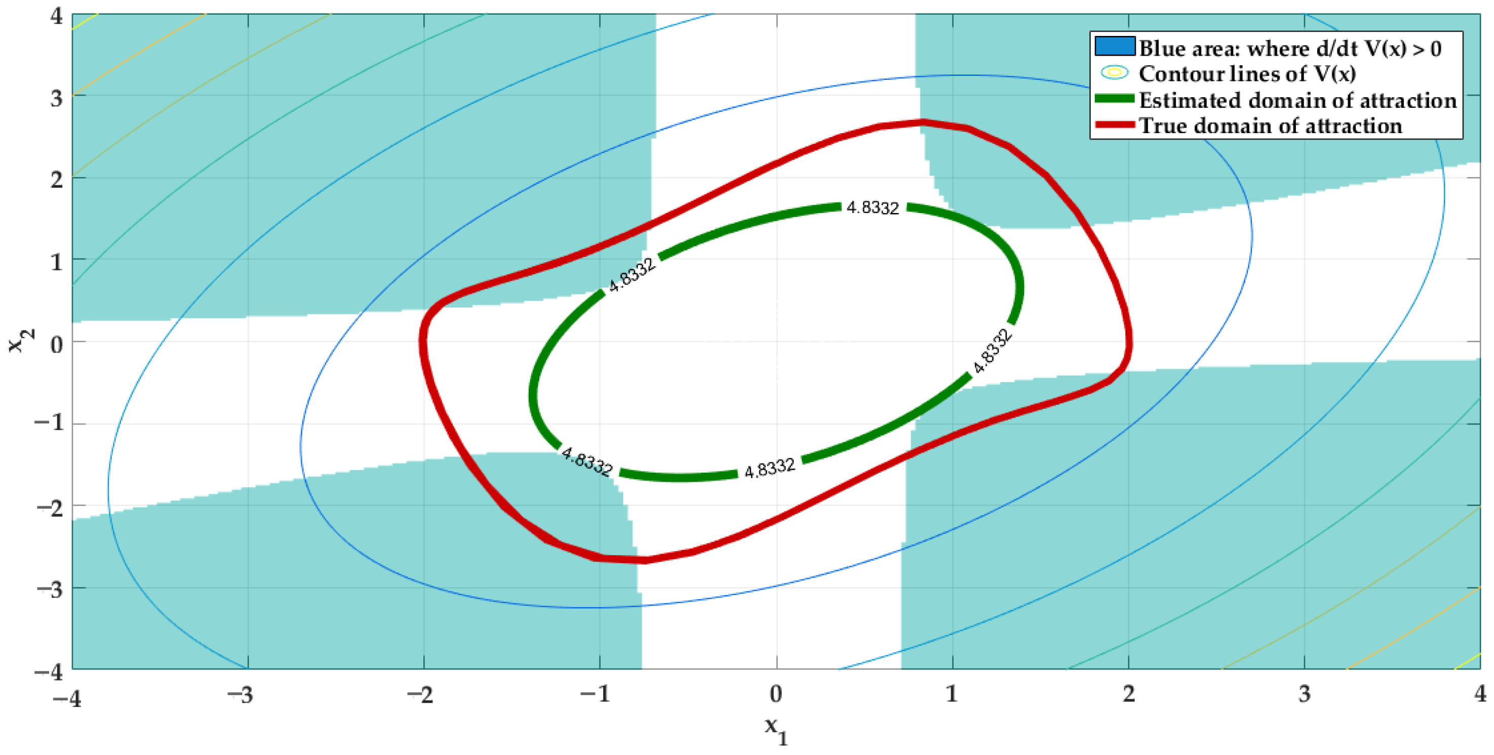
Consequently, the value of the radius domain is c ^ * = 4.8332 . The corresponding volume of the DA is Vol ( Ω c ( P 1 new ) ) = 2.1084 . The set of the domain is described as Ω c = { x R n : V 1 ( x ) = 3 x 1 2 1.98 x 1 x 2 + 2.0759 x 2 2 = 4.8332 } . Figure 2 shows the limit cycle in red and the level sets of the certifying LFs in green.
B.
Second loop:
Next, we consider the LF V 1 ( x ) = 3 x 1 2 1.98 x 1 x 2 + 2.0759 x 2 2 and then
V 1 ˙ ( x ) = V 1 ˙ ( x ) t = V 1 ( x ) x f ( x ) = 1.98 x 1 2 12.13 x 1 x 2 2.17 x 2 2 1.98 x 1 3 x 2 + 4.15 x 1 2 x 2 2 .
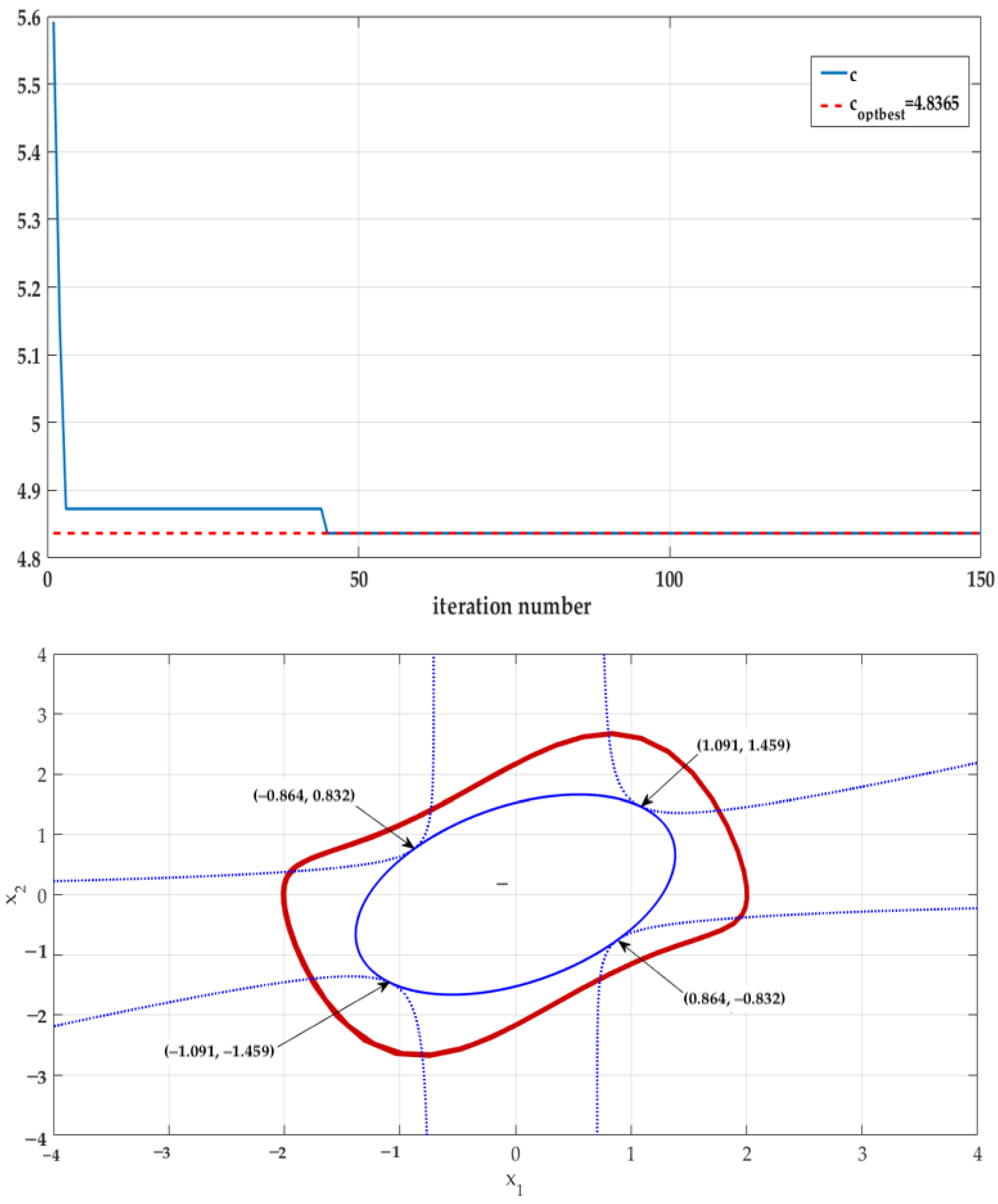
In this respect, we begin encoding variables whose particle position is specified about vector θ 1 ( x ( k ) ) = x ( k ) = [ x 1 ( k ) x 2 ( k ) ] . We state the LF as a fitness function of the Jaya algorithm given by V 1 ( x ( k ) ) = 3 ( x 1 ( k ) ) 2 1.98 x 1 ( k ) x 2 ( k ) + 2.0759 ( x 2 ( k ) ) 2 = c opt and then its derivative is V 1 ˙ ( x ( k ) ) = 1.98 ( x 1 ( k ) ) 2 12.13 x 1 ( k ) x 2 ( k ) 2.17 ( x 2 ( k ) ) 2 1.98 ( x 1 ( k ) ) 3 x 2 ( k ) + 4.15 ( x 1 ( k ) ) 2 ( x 2 ( k ) ) 2 < 0 . Subsequently, the proposed approach utilizing the Jaya algorithm ascertains the values of V 1 ( x opt ) , V ˙ 1 ( x opt ) and x opt = [ x 1 opt x 2 opt ] . Next, the parameter settings used for the Jaya algorithm are stated. The application of Algorithm 2, based on a population size of 50 and 150 iterations, provides the optimum solutions. These solutions belong to the line tangent to the DA obtained after evaluating the optimization outcome. Hence, we select the following:
x opt = 1.091 1.459 , 1.091 1.459 , 0.864 0.832 , 0.864 0.832 ,
and the radius value of the DA is c opt , best = 4.83654 . Figure 3 (top) illustrates the evolution of the radius value of the DA, and Figure 3 (bottom) depicts the optimum solutions and the level set of the best DA.
C.
DA using LF2:
We use the polynomial function V 2 ( x ) = ( θ 2 ( x ) ) P 2 θ 2 ( x ) , with
P 2 = a 1 a 2 0 0 0 a 2 a 3 0 0 0 0 0 a 4 a 5 a 6 0 0 a 5 a 7 a 8 0 0 a 6 a 8 a 9 .
Then, we have that
V 2 ( x ) = a 1 x 1 2 + 2 a 2 x 1 x 2 + a 3 x 2 2 + a 4 x 1 4 + 2 a 5 x 1 3 x 2 + ( 2 a 6 + a 7 ) x 1 2 x 2 2 + 2 a 8 x 1 x 2 3 + a 9 x 2 4 .
To determine a linear matrix decomposition as in the LMI given by (5), observe that the polynomial LF degree is four and the degree of the Van der Pol model is three. Thus, we obtain V 2 ˙ ( x ) with a degree d L that is equal to six. For instance, let q ( x ) be defined as q ( x ) = q 1 x 1 2 + 2 q 2 x 1 x 2 + q 3 x 2 2 . Then, the matrices D f ( α , P 2 ) , Z ( Q , P 2 ) and F ( Q , P 2 ) in (5) are given by
D f ( P 2 ) = 2 a 2 ( a 3 a 1 a 2 ) 0 0 0 0 0 0 0 * 2 ( a 2 + a 3 ) 0 0 0 0 0 0 0 * * 2 a 5 ( 2 a 6 + a 7 + a 2 2 a 4 a 5 ) 0 0 0 0 0 * * * ( 4 a 6 2 a 7 + 2 a 3 6 a 5 ) ( 2 a 6 a 7 + 2 a 9 3 a 8 ) 0 0 0 0 * * * * ( 2 a 8 4 a 9 ) 0 0 0 0 * * * * * 0 2 a 5 0 0 * * * * * * ( 4 a 6 + 2 a 7 ) 3 a 8 0 * * * * * * * 4 a 9 0 * * * * * * * * 0 , D f ( α ) = 0 0 0 α 1 α 2 α 3 α 4 + α 17 α 5 + α 20 α 6 + α 18 * 0 α 1 α 2 0 α 4 α 5 α 6 α 19 * * 2 α 3 α 17 α 7 0 α 8 α 9 + α 13 α 10 + α 12 * * * 2 ( α 7 + α 20 ) α 8 α 8 α 9 α 10 α 11 * * * * 2 α 19 α 13 α 12 α 11 0 * * * * * 0 2 a 5 α 14 α 15 * * * * * * 0 0 α 16 * * * * * * * 0 0 * * * * * * * * 0 , D f ( α , P 2 ) = D f ( P 2 ) + D f ( α ) , Q = q 1 q 2 q 2 q 3 , Z ( Q , P 2 ) = q 1 q 2 0 0 0 0 0 0 0 * q 3 0 0 0 0 0 0 0 * * β 1 β 2 0 0 0 0 0 * * 0 β 3 β 4 0 0 0 0 * * 0 0 β 5 0 0 0 0 * * 0 0 0 β 6 β 7 0 0 * * 0 0 0 0 β 8 β 9 0 * * 0 0 0 0 0 β 10 β 11 * * 0 0 0 0 0 0 β 12 , F ( Q , P 2 ) = 0 0 0 0 0 0 0 0 0 * 0 0 0 0 0 0 0 0 * * β 1 β 2 0 0 0 0 0 * * 0 β 3 β 4 0 0 0 0 * * 0 0 β 5 0 0 0 0 * * 0 0 0 β 6 β 7 0 0 * * 0 0 0 0 β 8 β 9 0 * * 0 0 0 0 0 β 10 β 11 * * 0 0 0 0 0 0 β 12 ,
with
β 1 = μ q 1 a 1 β 2 = μ q 1 a 2 + μ q 2 a 1 β 3 = μ q 1 a 3 + μ q 3 a 1 + 4 μ q 2 a 2 β 4 = μ q 2 a 3 + μ q 3 a 2 β 5 = μ q 3 a 3 β 6 = μ q 1 a 4 β 7 = μ q 1 a 5 + μ q 2 a 4 β 8 = μ q 3 a 4 + μ q 1 a 7 + 2 μ q 1 a 6 + 4 μ q 2 a 5 β 9 = μ q 1 a 8 + 2 μ q 2 a 6 + μ q 2 a 7 + μ q 3 a 5 β 10 = μ q 1 a 9 + 2 μ q 3 a 6 + μ q 3 a 7 + 4 μ q 2 a 5 β 11 = μ q 2 a 9 + μ q 3 a 9 β 12 = μ q 3 a 9 . .
For μ = 0.1 , the optimization problem stated in (4) to maximize the DA volume is solved by considering the evaluation of inequalities (5) and (6) and the iterative procedure of different steps, leading to
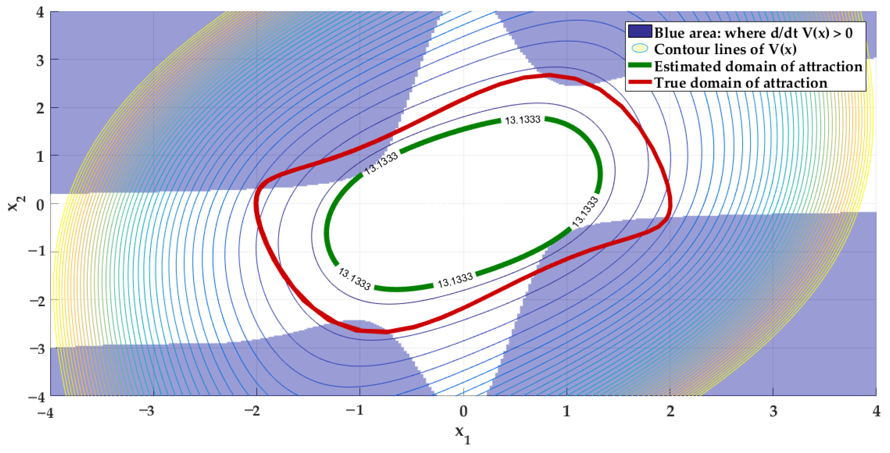
c ^ * = 13.1333 ,
P 2 = 3.9317 2.3438 0 0 0 2.3438 5 0 0 0 0 0 2.9422 0.7491 0.6947 0 0 0.7491 0.9190 0.5425 0 0 0.6947 0.5425 0.2048 ,
and
Ω c = { x R 2 : V 2 ( x ) = 3.9317 x 1 2 4.6876 x 1 x 2 + 5 x 2 2 + 2.9422 x 1 4 1.4982 x 1 3 x 2 + 2.3084 x 1 2 x 2 2 1.0850 x 1 x 2 3 + 0.2048 x 2 4 = 13.1333 }
Figure 4 shows the limit cycle and the level sets of the certifying LFs.
Then, we consider the LF given by
V 2 ( x ) = 3.9317 x 1 2 4.6876 x 1 x 2 + 5 x 2 2 + 2.9422 x 1 4 1.4982 x 1 3 x 2 + 2.3084 x 1 2 x 2 2 1.0850 x 1 x 2 3 + 0.2048 x 2 4 .
We calculate the derivative of V 2 ( x ) , with V ˙ 2 ( x ) = V 2 ( x ) / t = V 2 ( x ) / x f ( x ) . Hence, we begin encoding variables whose particle position is specified regarding the vector θ 2 ( x ( k ) ) = [ x 1 ( k ) x 2 ( k ) ( x 1 ( k ) ) 2 x 1 ( k ) x 2 ( k ) ( x 2 ( k ) ) 2 ] . We consider the LF as a fitness function of the Jaya algorithm stated as
V 2 ( x ( k ) ) = 3.9317 ( x 1 ( k ) ) 2 4.6876 x 1 ( k ) x 2 ( k ) + 5 ( x 2 ( k ) ) 2 + 2.9422 ( x 1 ( k ) ) 4 1.4982 ( x 1 ( k ) ) 3 x 2 ( k ) + 2.3084 ( x 1 ( k ) ) 2 ( x 2 ( k ) ) 2 1.0850 ( x 1 ( k ) ) ( x 2 ( k ) ) 3 + 0.2048 ( x 2 ( k ) ) 4 = c opt ,
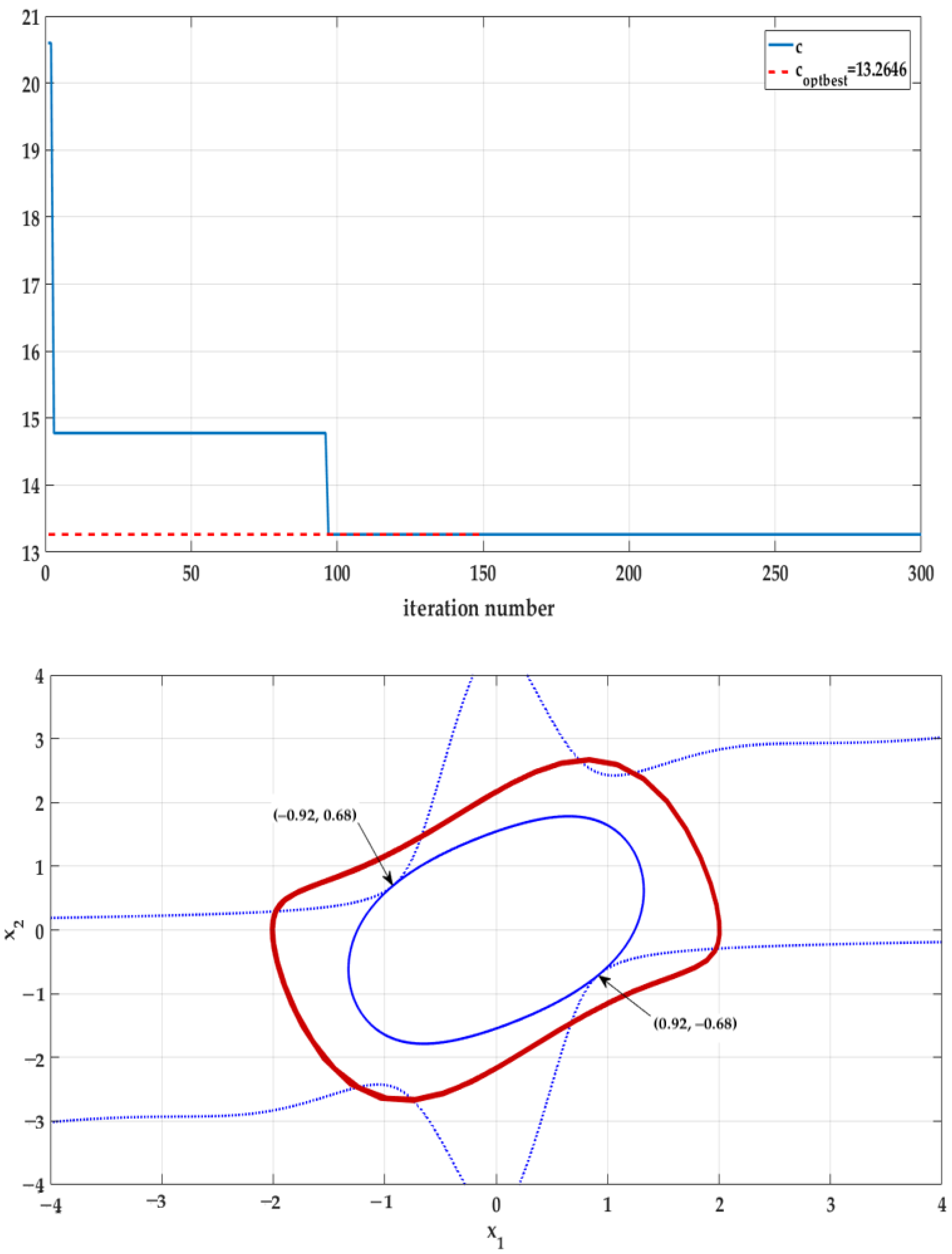
and its derivative given by V ˙ 2 ( x ( k ) ) = V 2 ( x ( k ) ) / t = V 2 ( x ( k ) ) / x f ( x ( k ) ) . Subsequently, the proposed approach uses the Jaya algorithm to ascertain the value of V 2 ( x opt ) , V ˙ 2 ( x opt ) , and x opt = [ x 1 opt x 2 opt ] . The parameter settings employed for the Jaya algorithm are the following. In the application of Algorithm 2, we utilize a population size of 50 and 150 iterations, giving the optimum solutions that belong to the line tangent to the DA.
Figure 5 (top) depicts the optimum solutions obtained after evaluating the optimization outcome. The following results are selected:
x opt = 0.92 0.68 , 0.92 0.68 .

4.3. Application 2

A significant feature of the compartmental modeling methods is that they are very commonly utilized. In particular, infectious diseases are often modeled mathematically using such methods. Therefore, in the compartmentalized analysis, the population is categorized according to the resulting labels: R, I, S, or recovered, infectious, or susceptible. As a rule of thumb, there is usually a flow pattern evident in the labels’ order, such as IESI, which indicates infectious, exposed, susceptible, and then infectious once again. These models date back to the early 20th century. Among the most important works are those of Kendall in 1956, Kermack and McKendrick in 1927, and Ross and Hudson in 1917. Most models are run based on deterministic ordinary differential equations. However, they can also be established using a stochastic mechanism. In turn, this seems more realistic but much more challenging to analyze. A model predicts how a disease will spread, how many people will be infected, or how long an epidemic will last.
In addition to these predictions, the model attempts to estimate various epidemiological factors, such as the reproductive rate. Using epidemic models, one can better understand how several public health actions impact the epidemic’s outcome. For example, how to issue a limited number of vaccines efficiently for an assumed population. For disease modeling, specifically for COVID-19’s investigation, the SIR model is typically used [47]. For decades, the dynamics of SIR models have been explored, examining chaos, bifurcation, and the stability problem analysis [48]. It is generally assumed that the recovery rate is constant in almost all research studies. However, the fact remains that the recovery rate depends on several considerations, including health system strategies, logistics, and medication availability. There has been a great deal of research in the past few years on models of systems described by differential equations with fractional operators [49]. It has also been noted that several works have investigated epidemic models with a fractional operator. This is so since they provide a comprehensive description of diseases from both physical and biological standpoints [48]. In this application, we use the advanced design technique of this current work. This enables us to evaluate the maximal DA in the context of an extended SIR epidemic model.
Many researchers have addressed the epidemic SIR model in the literature [50,51,52]. In mathematical epidemiology, the SIR model describes how an infectious disease spreads. In [53], the SIR model was used with
d S d t = A β S I d S + c I + δ R d I d t = β S I I d I α I c I d R d t = r I d R δ R ,
where S, I, and R are the numbers of susceptible, infectious, and recovered individuals from an infection, respectively. The total population is N = S + I + R . The constants A, c, d, r, α , β , δ are all positive constants. With A = 4 , c = d = r = α = β = γ = 0.5 and the shift of the rest position [ 4 1.6 0.8 ] . Then, the state space representation of the SIR model is formulated as
x ˙ 1 = 1.3 x 1 1.5 x 2 + 0.5 x 3 0.5 x 1 x 2 x ˙ 2 = 0.8 x 1 + 0.5 x 1 x 2 x ˙ 3 = 0.5 x 2 x 3 .
Using the system presented in (13), we could generate a fractional derivative epidemic model that may provide helpful insight into the COVID-19 pandemic [54].
As a second illustration of how our results may be applied, we assume the quadratic LF of second degree given by V 1 ( x ) = a 1 x 1 2 + 2 a 2 x 1 x 2 + 2 a 3 x 1 x 3 + a 4 x 2 2 + 2 a 5 x 2 x 3 + a 6 x 3 2 , with
P 1 = a 1 a 2 a 3 a 2 a 4 a 5 a 5 a 6 .
To determine a linear matrix decomposition as in (5), we calculate the derivative of LF. Note that the degree d L of V 1 ˙ ( x ) is equal to three. For instance, the degree of q ( x ) is 2 d q , and d q verifies the inequality defined in (2). Then, q ( x ) = q 1 x 1 2 + 2 q 2 x 1 x 2 + 2 q 3 x 1 x 3 + q 4 x 2 2 + 2 q 5 x 2 x 3 + q 6 x 3 2 , which implies d m = 2 . Vectors x { d v } , x { d n } and x { d m } are selected as x { d v } = x { d n } = [ x 1 x 2 x 3 ] x { d m } = [ x 1 x 2 x 3 x 1 2 x 1 x 2 x 1 x 3 x 2 2 x 2 x 3 x 3 2 ] , and D f ( x ) = ( x d m ) D f ( α , P ) ( x d m ) , D f ( α , P ) = D f ( α ) + D f ( P ) , with α being a vector of free parameters composed of 14 elements stated as α = [ α 1 α 2 α 3 α 4 α 5 α 6 α 7 α 8 α 9 α 10 α 11 α 12 α 13 α 14 ] . In addition, we have that D f ( α ) is a linear parametrization of the set Φ = { D f = D f : x { d m } D f ( α ) x { d m } = 0 , x R n } , with
D f ( α ) = 0 0 0 0 α 1 α 2 α 3 α 4 + α 14 α 5 * 0 0 α 1 α 3 α 4 0 α 6 α 8 * * 0 α 2 α 14 α 5 α 6 α 8 0 * * * 0 0 0 α 7 α 10 α 9 * * * * 2 α 7 α 10 0 α 12 α 11 * * * * * 2 α 9 α 12 α 11 0 * * * * * * 0 0 α 13 * * * * * * * 2 α 13 0 * * * * * * * * 0 .
The SMR of the polynomial d f ( x ) = V ( x ) / x f ( x ) is expressed as
D f ( P 2 ) = 2.6 a 1 + 1.6 a 2 ( 3 a 1 2.6 a 2 + 1.6 a 4 + a 3 ) ( a 1 2.6 a 3 + 1.6 a 5 2 a 3 ) 0 ( a 2 a 1 ) 0 0 ( a 5 a 3 ) 0 * ( a 5 3 a 2 ) ( a 2 3 a 3 2 a 5 + a 6 ) 0 ( a 4 a 2 ) 0 0 0 0 * * ( a 3 2 a 6 ) 0 0 0 0 0 0 * * * 0 0 0 0 0 0 * * * * 0 0 0 0 0 * * * * * 0 0 0 0 * * * * * * 0 0 0 * * * * * * * 0 0 * * * * * * * * 0 .
To compute Z ( x , Q , P 1 ) , we calculate the polynomial and represent it in the form of matrix Z ( x , Q , P 1 ) = ( 1 + μ V 1 ( x , P 1 ) ) q ( x ) . Hence, we have that
Q = q 1 q 2 q 3 q 2 q 4 q 5 q 3 q 5 q 6 = Q , Z ( Q , P 1 ) = [ Z 1 ( Q , P 1 ) , Z 2 ( Q , P 1 ) ] , Z 1 ( Q , P 1 ) = q 1 q 2 q 3 0 0 0 * q 4 q 5 0 0 0 * * q 6 0 0 0 * * * a 1 q 1 ( a 2 q 1 + a 1 q 2 ) ( a 3 q 1 + a 1 q 3 ) * * * * ( a 4 q 1 + a 2 q 4 + 4 a 1 q 4 ) 0 * * * * * ( a 6 q 1 + a 1 q 6 + 4 a 3 q 3 ) * * * * * * * * * * * * * * * * * * , Z 2 ( Q , P 1 ) = 0 0 0 0 0 0 0 0 0 0 ( a 5 q 1 + a 1 q 5 + 2 a 3 q 2 + 2 a 2 q 3 ) 0 a 4 q 2 + a 2 q 4 ( 2 a 5 q 2 + 2 a 2 q 5 + a 4 q 3 + a 3 q 4 ) ( 2 a 5 q 3 + 2 a 3 q 5 + a 6 q 2 + a 2 q 6 ) 0 0 ( a 6 q 3 + a 3 q 6 ) a 4 q 4 ( 2 a 5 q 4 + 2 a 4 q 5 ) 0 * ( a 6 q 4 + a 4 q 6 ) ( a 6 q 5 + a 5 q 6 ) * * a 6 q 6 .
Therefore, F ( Q , P 1 ) = [ F 1 ( Q , P 1 ) F 2 ( Q , P 1 ) ] , where
F 1 ( Q , P 1 ) = 0 0 0 0 0 0 * 0 0 0 0 0 * * 0 0 0 0 * * * a 1 q 1 ( a 2 q 1 + a 1 q 2 ) ( a 3 q 1 + a 1 q 3 ) * * * * ( a 4 q 1 + a 2 q 4 + 4 a 1 q 4 ) 0 * * * * * ( a 6 q 1 + a 1 q 6 + 4 a 3 q 3 ) * * * * * * * * * * * * * * * * * * , F 2 ( Q , P 1 ) = 0 0 0 0 0 0 0 0 0 0 ( a 5 q 1 + a 1 q 5 + 2 a 3 q 2 + 2 a 2 q 3 ) 0 a 4 q 2 + a 2 q 4 ( 2 a 5 q 2 + 2 a 2 q 5 + a 4 q 3 + a 3 q 4 ) ( 2 a 5 q 3 + 2 a 3 q 5 + a 6 q 2 + a 2 q 6 ) 0 0 ( a 6 q 3 + a 3 q 6 ) a 4 q 4 ( 2 a 5 q 4 + 2 a 4 q 5 ) 0 * ( a 6 q 4 + a 4 q 6 ) ( a 6 q 5 + a 5 q 6 ) * * a 6 q 6 .
A.
First loop:
The following vector is initially used for variable encoding pertaining to a particle position:
P 1 ( k ) = a 1 ( k ) a 2 ( k ) a 3 ( k ) * a 4 ( k ) a 5 ( k ) * * a 6 ( k ) .
Note that the pseudocode illustrates how we could determine the fitness value. This happens when we use Theorem 2 to calculate the maximum c for which the GEVP optimization method is feasible. The population size is 50, and the stopping condition is the highest number of iterations I max = 150 . To finish the five steps of the Jaya algorithm described in Section 3, by solving the LMI objective in (5) and (6) with μ = 0.1 , we obtain
P 1 ( k ) = 1.5111 0.9799 0.4883 0.9799 5.0000 0.0241 0.4883 0.0241 0.9353 .
Then, the DA is described as Ω c = { x R 3 : V 1 ( x ) = 1.5111 x 1 2 + 1.9598 x 1 x 2 + 0.9766 x 1 x 3 + 5 x 2 2 + 0.0482 x 2 x 3 + 0.9353 x 3 2 = 9.2810 } .
B.
Second loop:
We consider the LF stated as V 1 ( x ) = 1.5111 x 1 2 + 1.9598 x 1 x 2 + 0.9766 x 1 x 3 + 5 x 2 2 + 0.0482 x 2 x 3 + 0.9353 x 3 2 . We calculate the derivative of V ( x ) , with V 1 ˙ ( x ) = V 1 ( x ) / t = V 1 ( x ) / x f ( x ) , obtaining
V 1 ˙ ( x ) = 2.361 x 1 2 + 1.4073 x 1 x 2 0.6965 x 1 x 3 2.9156 x 2 2 + 0.4021 x 1 x 3 1.3823 x 3 2 0.5312 x 1 2 x 2 + 4.0201 x 1 x 2 2 0.4642 x 1 x 2 x 3
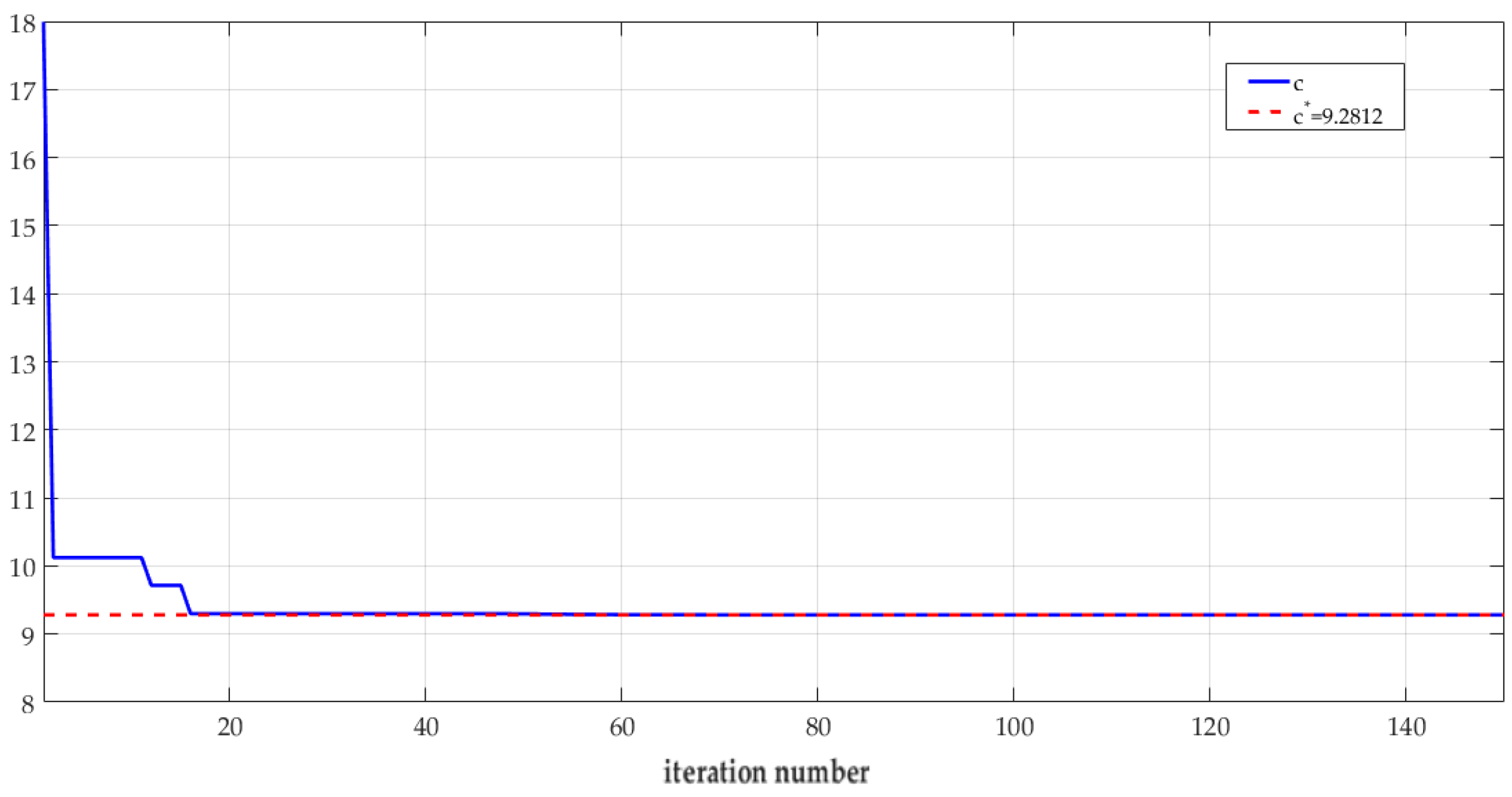
Hence, we begin encoding variables whose particle position is specified concerning the vector θ 1 ( x ( k ) ) = x ( k ) = [ x 1 ( k ) x 2 ( k ) x 3 ( k ) ] . Using Algorithm 2, with a population size of 50 and a maximum number of iterations of 150, the optimal solution is x opt = [ 1.5981 1.4426 0.4256 ] . Figure 6 illustrates the evolution of c.

4.4. Discussion

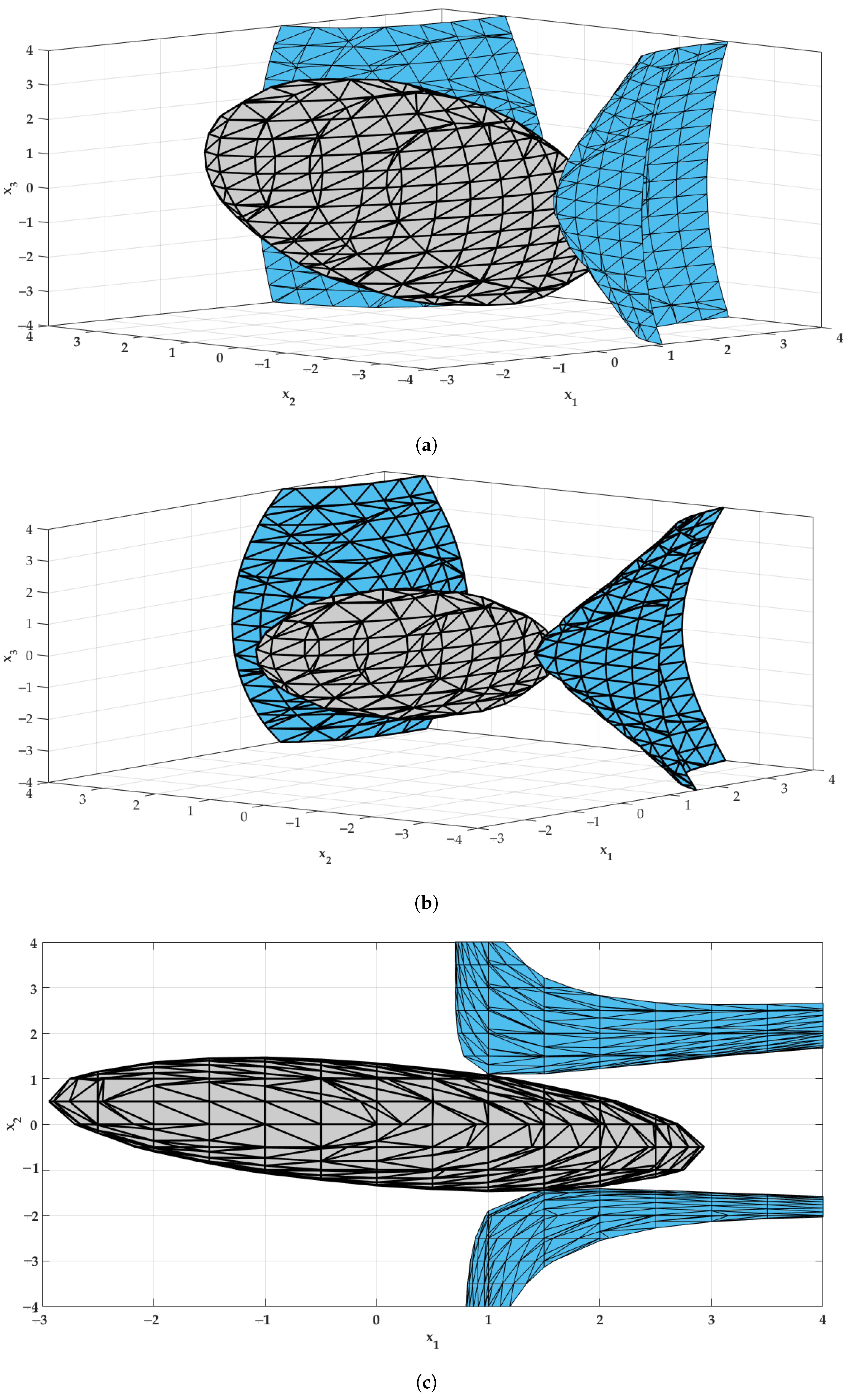
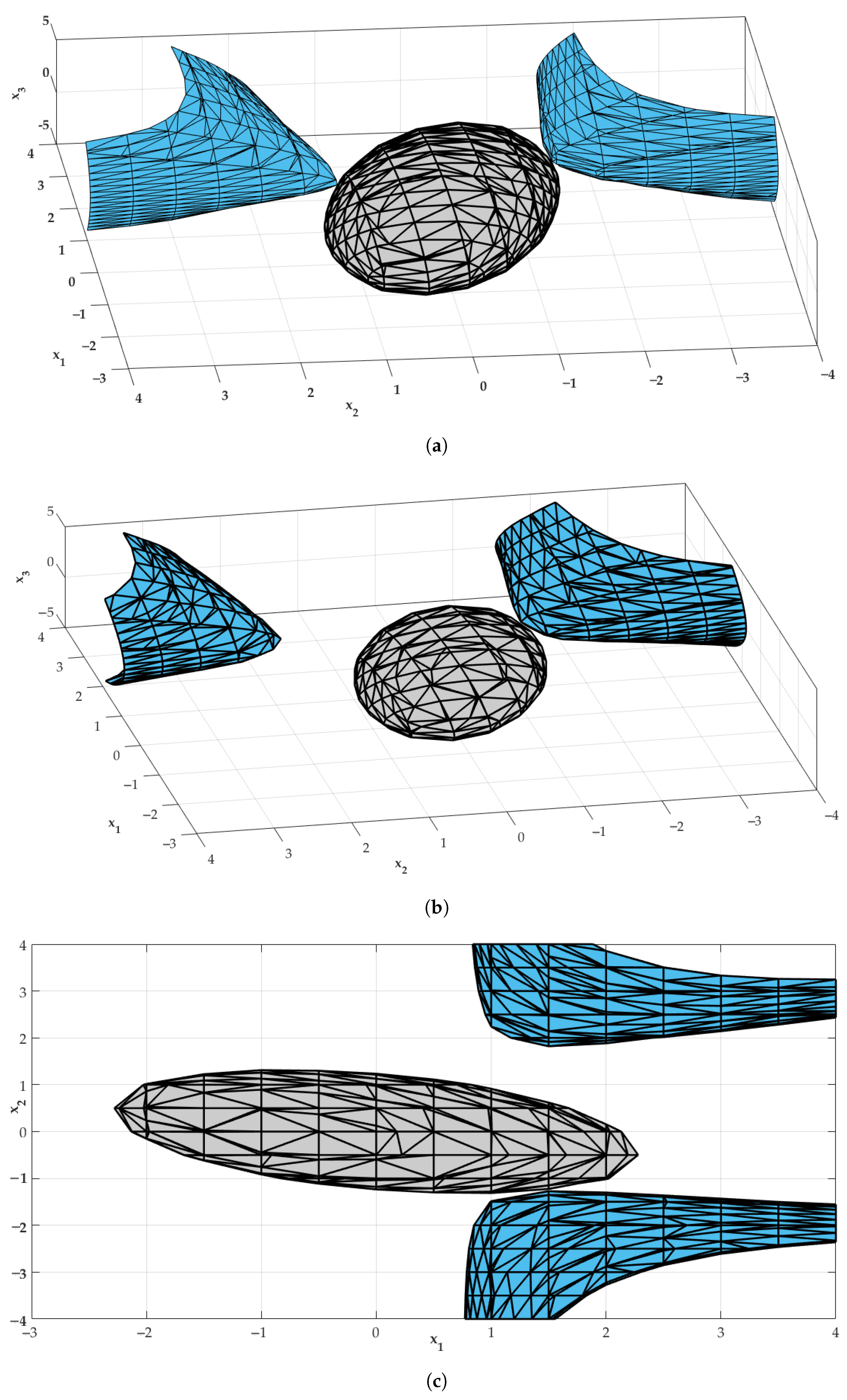
Next, we analyze the performance of the presented methods using the Van der Pol and SIR models. Several criteria were used to assess the efficiency of the developed method: the DA volume, computation time, and method’s ability to identify the tangency point (defined here as the DA problem’s optimal solution). Table 1 compares the DA features of our method with benchmark methods presented in [21,38,53]. Note that the DA volume was considered the primary criterion to establish the comparison. The two second-order methods introduced in [21,38] used the LF stated in (12) for the Van der Pol model. The third-order method presented in [53] utilized the LF defined in (14) for the SIR model. Observe that the obtained results confirmed the superiority of our method as it offered vastly greater DA volumes. Also, our method provided an algorithm that maximized the DA while allowing the computation of a specific LF. Moreover, our algorithm established an explicit LF. Using our method, a primary DA was identified and then enlarged until the tangency point between the LF and its derivative, which was accurately determined. This numerical analysis proved that the proposed algorithm led to the optimal solution and accurately specified the searched tangency point. Note that the implementation remained straight and significantly reduced the computation time. No random analysis, initialization, or searching were needed. By running the step-by-step algorithm definitively led to the same results independently from the initialization step. Observe that running our algorithm avoided dummy solutions, which is not all the time the case for the second-order models presented in [21,38]. The third-order model was studied to generalize the satisfactory performance of the proposed method to estimate the DA. The same highlighted performance as the previous discussion is confirmed for the example studied in Figure 5 (bottom). The DA volume was significantly greater, and the tangency point was accurately fixed. In contrast, the method stated in [53] did not guarantee this latter outcome. Figure 7 displays a 3D view of the original plot (a) of the DA estimated by the proposed method for the SIR model, a 3D view that was rotated to visualize the tangency point better (b), and its corresponding 2D plot (c). Figure 8 shows a 3D view of the original plot (a) of the DA estimated by the method given in [53] for the SIR model, a 3D view that was rotated to visualize the tangency point better (b), and its corresponding 2D plot (c).

5. Conclusions

In this article, we provided a metaheuristic-based solution for stability analysis of nonlinear systems. of these systems by combining two optimization phases. This set was in a definite negative region of the time derivative for a polynomial LF. Then, we considered a global optimization problem stated in two phases, where the first phase was an external optimization to search for a definite positive LF, and the second phase was an internal optimization to ensure an accurate estimate of the attraction region for each candidate LF that was optimized externally. We used a Jaya optimization to provide an efficient way to characterize accurately the volume and shape of the maximal DAs. We conducted numerical experiments to validate the proposed approach and provided two potential real-world applications related to the Van der Pol oscillator and a SIR epidemic model.
Specifically, this article discussed benchmarking results of referential techniques, which aim to recommend numerical methods for estimating the DA of nonlinear dynamical autonomous systems. In this respect, the method examined in this work was applied to calculate optimal quadratic LFs in the neighborhood of asymptotically stable equilibrium points. The principal addressed concept in this article consisted in estimating the largest DA belonging to the best level set of an LF, which was assumed to be entirely included in the domain of negative definiteness of the LF and its corresponding time derivative. We combined n analytical technique with a random searching method. Then, a metaheuristic optimization method was employed to enhance the performance of the current design. This allowed an accurate computed estimation of the DA size and an explicit analytical expression representing its geometrical form. As part of the optimization strategy, a tangency constraint was examined in relation to the constraints on the sign of the LF and its level sets. Such constraints ensured a maximal DA around the asymptotic stable equilibrium.
The developed method in the present investigation was applied to both polynomial nonlinear autonomous systems with second and third degrees. One distinctive feature of the designed technique in this article is that it can estimate the DA more efficiently than the other presented techniques in the literature. The numerical simulation analysis proved that the DAs obtained by the proposed method allowed us to estimate the stability domains with satisfactory results in shape and volume. The reached results can be beneficial for real-time control designs. In addition, the synthesized algorithms can help control problems using the online sequential composition hypothesis. Future work should be to explore applying the studied techniques to real plants. In particular, the design of enlarged DAs will be economically beneficial for most physical processes.

Author Contributions

Conceptualization, H.A., H.J., F.H. and D.P.; methodology, F.H. and H.J.; software, H.J.; validation, D.P., V.L. and W.R.; formal analysis, F.H. and H.J.; investigation, H.J.; resources, H.J.; data curation, H.J. and V.L.; writing—original draft preparation, F.H. and H.J.; writing—review and editing, V.L.; visualization, D.P. and F.H.; supervision, H.J. and V.L.; project administration F.H., H.J., D.P., and W.R.; funding acquisition, H.J. All authors have read and agreed to the published version of the manuscript.

Funding

This research was funded by the Research Deanship of Hail University, KSA (Project Number RG-21 127).

Data Availability Statement

Not applicable.

Acknowledgments

The authors would also like to thank the reviewers for their constructive comments, which led to improvement in the presentation of the manuscript.

Conflicts of Interest

The authors declare that they have no conflict of interest.

References

  1. Nersesov, S.G.; Ashrafiuon, H.; Ghorbanian, P. On estimation of the domain of attraction for sliding mode control of underactuated nonlinear systems. Int. J. Robust Nonlinear Control 2014, 24, 811–824. [Google Scholar] [CrossRef]
  2. Khalil, H.K. Nonlinear Systems; Prentice-Hall: Upper Saddle River, NJ, USA, 2002. [Google Scholar]
  3. Jerbi, H. Estimations of the domains of attraction for classes of nonlinear continuous polynomial systems. Arab. J. Sci. Eng. 2017, 42, 2829–2837. [Google Scholar] [CrossRef]
  4. Wang, C.; Zhu, T.; Chen, Y. Stability analysis of the nabla distributed-order nonlinear systems. Fractal Fract. 2022, 6, 228. [Google Scholar] [CrossRef]
  5. Agarwal, R.; Hristova, S.; O’Regan, D. Stability of generalized proportional Caputo fractional differential equations by Lyapunov functions. Fractal Fract. 2022, 6, 34. [Google Scholar] [CrossRef]
  6. Hamidi, F.; Jerbi, H.; Aggoune, W.; Djemai, M.; Abdelkrim, M.N. Enlarging the domain of attraction in nonlinear polynomial systems. Int. J. Comput. Commun. Control 2013, 8, 538–547. [Google Scholar] [CrossRef] [Green Version]
  7. Charfeddine, M.; Jouili, K.; Jerbi, H.; Braiek, N.B. Output tracking control design for non-minimum phase systems: Application to the ball and beam model. Int. Rev. Autom. Control 2011, 4, 47–55. [Google Scholar]
  8. Lam, H.K. Stabilization of nonlinear systems using sampled-data output-feedback fuzzy controller based on polynomial-fuzzy-model-based control approach. IEEE Trans. Syst. Man Cybern. B 2011, 42, 258–267. [Google Scholar] [CrossRef]
  9. Vannelli, A.; Vidyasagar, M. Maximal Lyapunov functions and domains of attraction for autonomous nonlinear systems. Automatica 1985, 21, 69–80. [Google Scholar] [CrossRef]
  10. Genesio, R.; Tartaglia, M.; Vicino, A. On the estimation of asymptotic stability regions: State of the art and new proposals. IEEE Trans. Autom. Control 1985, 30, 747–755. [Google Scholar] [CrossRef] [Green Version]
  11. Pitarch, J.L.; Sala, A.; Arino, C.V. Closed-form estimates of the domain of attraction for nonlinear systems via fuzzy-polynomial models. IEEE Trans. Cybern. 2014, 4, 526–538. [Google Scholar] [CrossRef] [Green Version]
  12. Chesi, G.; Colaneri, P. Homogeneous rational Lyapunov functions for performance analysis of switched systems with arbitrary switching and dwell time constraints. IEEE Trans. Autom. Control 2017, 62, 5124–5137. [Google Scholar] [CrossRef]
  13. Ghaoui, L.E.; Scorletti, G. Control of rational systems using linear-fractional representations and linear matrix inequalities. Automatica 1996, 9, 1273–1284. [Google Scholar] [CrossRef]
  14. Kokossis, A.C.; Floudas, C.A. Stability in optimal design: Synthesis of complex reactor networks. AICHE J. 1994, 5, 849–861. [Google Scholar] [CrossRef]
  15. Monnigmann, M.; Marquardt, W. Steady-state process optimization with guaranteed robust stability and feasibility. AICHE J. 2003, 12, 3110–3126. [Google Scholar] [CrossRef]
  16. Rahman, M.Z.U.; Liaquat, R.; Rizwan, M.; Martin-Barreiro, C.; Leiva, V. A robust controller of a reactor electromicrobial system based on a structured fractional transformation for renewable energy. Fractal Fract. 2022, 6, 736. [Google Scholar] [CrossRef]
  17. Rahman, M.Z.U.; Leiva, V.; Martin-Barreiro, C.; Mahmood, I.; Usman, M.; Rizwan, M. Fractional transformation-based intelligent H-infinity controller of a direct current servo motor. Fractal Fract. 2023, 7, 29. [Google Scholar] [CrossRef]
  18. Ringertz, U.T. Eigenvalues in optimum structural design. In Large-Scale Optimization with Applications; Springer: New York, NY, USA, 1997; pp. 135–149. [Google Scholar]
  19. Chermnykh, S.V. Carleman Linearization and normal forms for differential systems with quasiperiodic coefficients. Springer Plus 2016, 5, 1347. [Google Scholar] [CrossRef] [Green Version]
  20. Banks, S.P.; Hernandez, C.N. A new proof of McCann’s theorem and the generalization of Lyapunov’s equation to non-linear systems. Int. J. Innov. Comput. Inf. Control 2005, 1, 1–16. [Google Scholar]
  21. Hachicho, O. A novel LMI-based optimization algorithm for the guaranteed estimation of the domain of attraction using rational Lyapunov functions. J. Frankl. Inst. 2007, 344, 535–552. [Google Scholar] [CrossRef]
  22. Chesi, G. Estimating the domain of attraction via union of continuous families of Lyapunov estimates. Syst. Control Lett. 2007, 56, 326–333. [Google Scholar] [CrossRef]
  23. Chesi, G. Estimating the domain of attraction for non-polynomial systems via LMI optimizations. Automatica 2009, 45, 1536–1541. [Google Scholar] [CrossRef]
  24. Chesi, G.; Garulli, A.; Tesi, A.; Vicino, A. Solving quadratic distance problems: An LMI-based approach. IEEE Trans. Autom. Control 2003, 48, 200–212. [Google Scholar] [CrossRef]
  25. Chesi, G. Optimal representation matrices for solving polynomial systems via LMI. Int. J. Pure Appl. Math. 2008, 45, 397–412. [Google Scholar]
  26. Guerra, T.M.; Vermeiren, L. LMI-based relaxed nonquadratic stabilization conditions for nonlinear systems in the Takagi-Sugeno form. Automatica 2004, 40, 823–829. [Google Scholar] [CrossRef]
  27. Lam, H.K.; Leung, F.H. LMI-based stability and performance conditions for continuous-time nonlinear systems in the Takagi-Sugeno form. IEEE Trans. Syst. Man Cybern. B 2007, 37, 1396–1406. [Google Scholar] [CrossRef]
  28. Wu, F.; Prajna, S. SOS-based solution approach to polynomial LPV system analysis and synthesis problems. Int. J. Control 2005, 78, 600–611. [Google Scholar] [CrossRef]
  29. Chesi, G. On the gap between positive polynomials and SOS of polynomials. IEEE Trans. Autom. Control 2007, 52, 1066–1072. [Google Scholar] [CrossRef] [Green Version]
  30. Hamidi, F.; Aloui, M.; Jerbi, H.; Kchaou, M.; Abbassi, R.; Popescu, D.; Ben Aoun, S.; Dimon, C. Chaotic particle swarm optimisation for enlarging the domain of attraction of polynomial non-linear systems. Electronics 2020, 9, 1704. [Google Scholar] [CrossRef]
  31. Hamidi, F.; Jerbi, H.; Olteanu, S.C. An enhanced stabilizing strategy for switched nonlinear systems. Stud. Inform. Control 2019, 4, 391–400. [Google Scholar] [CrossRef]
  32. Matallana, L.G.; Blanco, A.M.; Bandoni, J.A. Estimation of domains of attraction: A global optimization approach. Math. Comput. Model. 2010, 5, 2574–2585. [Google Scholar] [CrossRef] [Green Version]
  33. Matallana, L.G.; Blanco, A.M.; Bandoni, J.A. Nonlinear dynamic systems design based on the optimization of the domain of attraction. Math. Comput. Model. 2011, 6, 731–745. [Google Scholar] [CrossRef]
  34. Hashemzadeh, F.; Yazdanpanah, M. Semi-global enlargement of domain of attraction for a class of affine nonlinear systems. In Proceedings of the IEEE International Conference on Control Applications, Munich, Germany, 4–6 October 2006; Volume 4776991, pp. 2257–2262. [Google Scholar]
  35. Sadat, E.; Shahri, A.; Alfi, A.; Machado, J.A.T. An extension of estimation of domain of attraction for fractional order linear system subject to saturation control. Appl. Math. Lett. 2015, 47, 26–34. [Google Scholar]
  36. Huang, M.; Lu, S.; Shateyi, S.; Saberi-Nik, H. Ultimate boundedness and finite time stability for a high dimensional fractional-order Lorenz model. Fractal Fract. 2022, 6, 630. [Google Scholar] [CrossRef]
  37. Houssein, E.H.; Gad, A.G.; Wazery, Y.M. Jaya algorithm and applications: A comprehensive review. In Metaheuristics and Optimization in Computer and Electrical Engineering; Springer: Berlin/Heidelberg, Germany, 2021; pp. 3–24. [Google Scholar]
  38. Najafi, E.; Babuška, R.; Lopes, G. A fast sampling method for estimating the domain of at-traction. Nonlinear Dyn. 2016, 2, 823–834. [Google Scholar] [CrossRef]
  39. Lam, H.K.; Seneviratne, L.D. BMI-based stability and performance design for fuzzy-model-based control systems subject to parameter uncertainties. IEEE Trans. Syst. Man Cybern. B 2004, 3, 502–514. [Google Scholar] [CrossRef]
  40. Aloui, M.; Hamidi, F.; Jerbi, H.; Omri, M.; Popescu, D.; Abbassi, R. A chaotic krill herd optimization algorithm for global numerical estimation of the attraction domain for nonlinear systems. Mathematics 2021, 9, 1743. [Google Scholar] [CrossRef]
  41. Ramirez-Figueroa, J.A.; Martin-Barreiro, C.; Nieto, A.B.; Leiva, V.; Galindo-Villardón, M.P. A new principal component analysis by particle swarm optimization with an environmental application for data science. Stoch. Environ. Res. Risk Assess. 2021, 35, 1969–1984. [Google Scholar] [CrossRef]
  42. Charfeddine, S.; Alharbi, H.; Jerbi, H.; Kchaou, M.; Abbassi, R.; Leiva, V. A stochastic optimization algorithm to enhance controllers of photovoltaic systems. Mathematics 2022, 10, 2128. [Google Scholar] [CrossRef]
  43. Chaouch, H.; Charfeddine, S.; Ben Aoun, S.; Jerbi, H.; Leiva, V. Multiscale monitoring using machine learning methods: New methodology and an industrial application to a photovoltaic system. Mathematics 2022, 10, 890. [Google Scholar] [CrossRef]
  44. FitzHugh, R. Impulses and physiological states in theoretical models of nerve membranes. Internat. Biophys. J. 1961, 1, 445–466. [Google Scholar] [CrossRef] [Green Version]
  45. Nagumo, J.; Arimoto, S.; Yoshizawa, S. An active pulse transmission line simulating nerve axon. Proceeding IRE 1962, 50, 2061–2070. [Google Scholar] [CrossRef]
  46. Cartwright, J.H.; Eguíluz, V.M.; Hernández-García, E.; Piro, O. Dynamics of elastic excitable media. Int. J. Bifurc. Chaos 1999, 9, 2197–2202. [Google Scholar] [CrossRef] [Green Version]
  47. Anand, N.; Sabarinath, A.; Geetha, S.; Somanath, S. Predicting the spread of COVID-19 using SIR model augmented to incorporate quarantine and testing. Trans. Indian Natl. Acad. Eng. 2020, 2, 141–148. [Google Scholar] [CrossRef]
  48. Tang, Y.; Huang, D.; Ruan, S.; Zhang, W. Coexistence of limit cycles and homoclinic loops in a SIRS model with a nonlinear incidence rate. SIAM J. Appl. Math. 2008, 2, 621–639. [Google Scholar] [CrossRef]
  49. Zhang, Z.; Jain, S. Mathematical model of Ebola and COVID-19 with fractional differential operators: Non-Markovian process and class for virus pathogen in the environment. Chaos Solitons Fractals 2020, 140, 110175. [Google Scholar] [CrossRef]
  50. Zhang, Y.; Ma, X.; Din, A. Stationary distribution and extinction of a stochastic SEIQ epidemic model with a general incidence function and temporary immunity. AIMS Math. 2021, 6, 12359–12378. [Google Scholar] [CrossRef]
  51. Ushirobira, R.; Efimov, D.; Blirnan, P.A. Estimating the infection rate of a SIR epidemic model via differential elimination. In Proceedings of the 18th European Control Conference, Naples, Italy, 25–28 June 2019; pp. 1170–1175. [Google Scholar]
  52. Harko, T.; Lobo, F.S.; Mak, M. Exact analytical solutions of the susceptible-infected-recovered (SIR) epidemic model and of the SIR model with equal death and birth rates. Appl. Math. Comput. 2014, 236, 184–194. [Google Scholar] [CrossRef] [Green Version]
  53. Warthenpfuhl, S.A. Stabilitätsanalyse für Nichtlineare Systeme Mithilfe der Interval-Larithmetik. Ph.D. Thesis, Universität Wuppertal, Wuppertal, Germany, 2012. [Google Scholar]
  54. Rangasamy, M.; Chesneau, C.; Martin-Barreiro, C.; Leiva, V. On a novel dynamics of SEIR epidemic models with a potential application to COVID-19. Symmetry 2022, 14, 1436. [Google Scholar] [CrossRef]
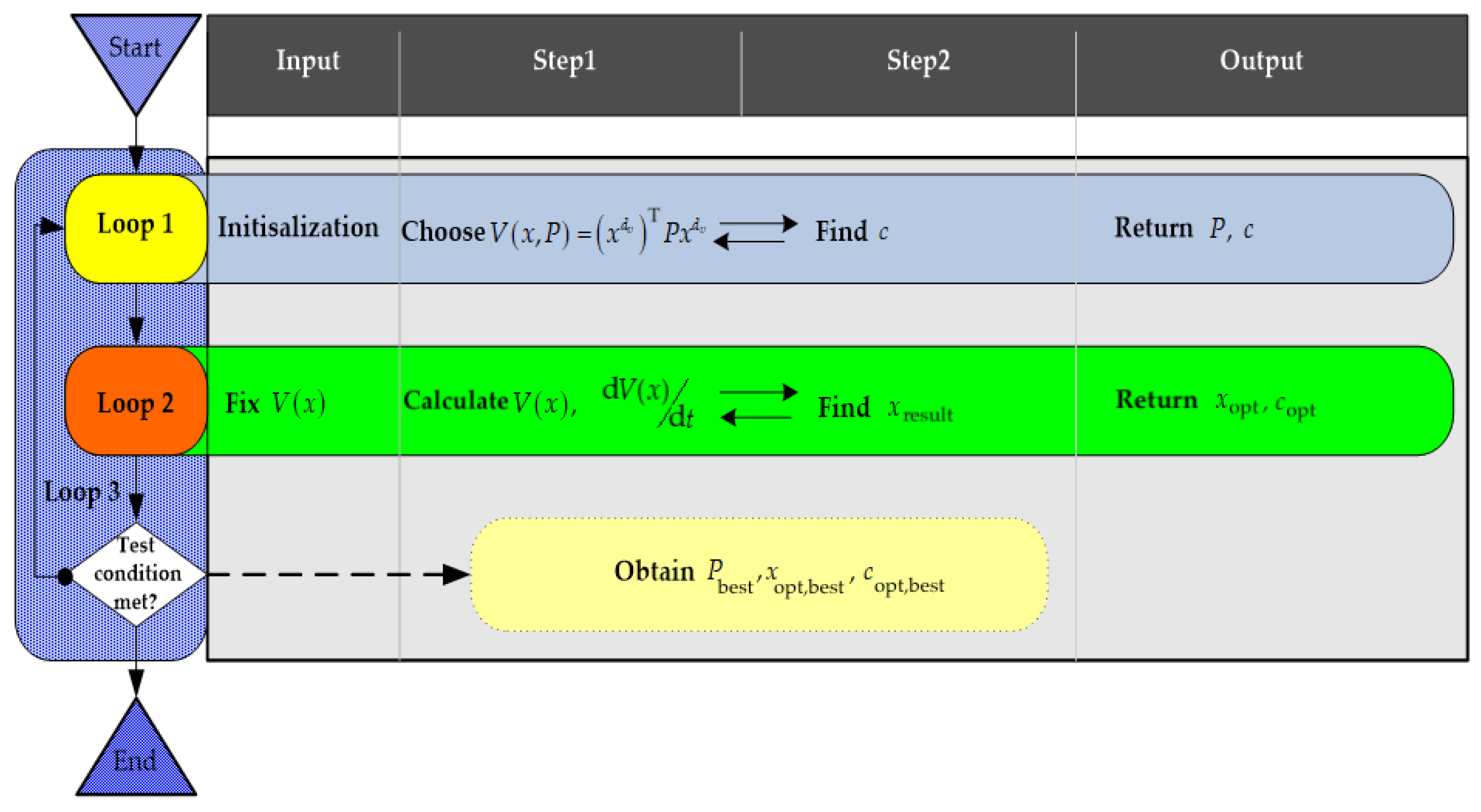
Figure 1. Workflow of the global algorithm.
Fractalfract 07 00078 g001
Figure 2. DA from the first loop.
Fractalfract 07 00078 g002
Figure 3. Iterative variation of c using the method with a quadratic LF for the Van der Pol application (top) and DA and optimum state solution (bottom).
Fractalfract 07 00078 g003
Figure 4. DA and optimum state solution.
Fractalfract 07 00078 g004
Figure 5. Iterative variation of c using the method with a quadratic LF for the Van der Pol application (top) and DA and optimum state solution (bottom).
Fractalfract 07 00078 g005
Figure 6. Iterative variation of c ^ * for the SIR application.
Fractalfract 07 00078 g006
Figure 7. Plots of a 3D view of the original structure (a), a 3D view that was rotated to visualize the tangency point better (b), and its corresponding 2D plot (c) of the DA estimated by the proposed method for the SIR model, with V ( P , c ) displayed in gray and d V ( P , c ) / d t in blue.
Fractalfract 07 00078 g007
Figure 8. Plots of a 3D view of the original structure (a), a 3D view that was rotated to visualize the tangency point better (b), and its corresponding 2D plot (c) of the DA estimated by the method given in [53] for the SIR model, with V ( P , c ) displayed in gray and d V ( P , c ) / d t in blue.
Fractalfract 07 00078 g008
Table 1. Comparative analysis of the proposed method and methods presented in [21,38,53].
ApplicationStudied SystemMethodLFFeatures of the DA
Van der Pol x ˙ 1 = x 2 Proposed V ( x ) = 3 x 1 2 1.98 x 1 x 2 + 2.0759 x 2 2 c opt = 4.8365 , Vol = 2.113
x ˙ 2 = x 1 x 2 + x 1 2 x 2 Given in [21] V ( x ) = 1.5 x 1 2 x 1 x 2 + x 2 2 c opt = 2.09 , Vol = 1.8694
Given in [38] V ( x ) = 1.5 x 1 2 x 1 x 2 + x 2 2 c opt = 2.318 , Vol = 2.0733
SIR model x ˙ 1 = 1.3 x 1 1.5 x 2 + 0.5 x 3 0.5 x 1 x 2 Proposed V ( x ) = 1.5111 x 1 2 + 1.9598 x 1 x 2 + 0.9766 x 1 x 3 c opt = 9.2812 , Vol = 12.6469
x ˙ 2 = 0.8 x 1 + 0.5 x 1 x 2 + 5 x 2 2 + 0.0482 x 2 x 3 + 0.9353 x 3 2
x ˙ 3 = 0.5 x 2 x 3 Given in [53] V ( x ) = 0.6295 x 1 2 + 0.7958 x 1 x 2 + 0.4084 x 1 x 3 c opt = 2.6094 , Vol = 6.0483
+ 1.6992 x 2 2 + 0.3874 x 2 x 3 + 0.6021 x 3 2
Disclaimer/Publisher’s Note: The statements, opinions and data contained in all publications are solely those of the individual author(s) and contributor(s) and not of MDPI and/or the editor(s). MDPI and/or the editor(s) disclaim responsibility for any injury to people or property resulting from any ideas, methods, instructions or products referred to in the content.