LFM Signal Parameter Estimation via FTD-FRFT in Impulse Noise

Abstract

LFM signals are widely applied in radar, communication, sonar and many other fields. LFM signals received by these systems contain a lot of noise and outliers. In order to suppress the interference of strong impulse noise on target signals and realize the accurate estimation of LFM signal parameters, the impulse noise of echo signals need to be filtered. In this paper, to solve the problem of poor performance of LFM signal parameter estimation based on fractional Fourier transform in impulse noise, alpha stable distribution is used to establish the mathematical model of impulse noise. The proposed fastest tracking differentiator with an adaptive tracking factor is used to suppress the strong impulse noise, and fractional Fourier transform is used to estimate the parameter of the LFM signals. The experimental results show that the proposed fastest tracking differentiator with an adaptive tracking factor has a good filtering performance. It can effectively filter the impulse noise in the echo signal and allows the FrFT method to accurate estimate the parameters of the LFM signals in strong impulse noise.

1. Introduction

Linear frequency modulation (LFM) signals have high resolution and large time-bandwidth product. They have been widely applied in radar, communication, sonar and many other fields [1,2,3,4]. However, LFM signals often encounter interference by different noise sources, and it is difficult to estimate the parameters of LFM signals. Therefore, the parameter estimation of LFM signals has become a hot issue in the field of signal processing [5,6,7,8,9]. Gaussian distribution obeys the generalized central limit theorem, so the traditional parameter estimation methods of LFM signals assume that the background noise obeys Gaussian distribution. Accordingly, many time-frequency analysis tools can be used to estimate the parameters of LFM signals in Gaussian noise. However, there are many stochastic noises in real environments, which may have sharp spikes or occasional bursts different from what one would expect from Gaussian distribution.

In [10], it was demonstrated that noise on a telephone line can be described by alpha stable distribution. In [11], it was indicated that alpha stable distribution is an ideal model that can be used to describe atmospheric noise. In [12], it was proved that alpha stable distribution is consistent with multi-path interference in wireless networks and radar backscatter echoes. In [13], it was shown that the background noise commonly assumed as Gaussian may not truly represent the effect of human activities on noise characteristics in broadband power-line communications. Symmetric alpha stable processes can be used to model the background noise of power-line communications. Hence, they have great theoretical and practical significance for research on the parameter estimation methods of LFM signals in impulse noise.

The probability density function of alpha stable distribution has heavy tailing, which is more consistent with noise with significant impulse characteristics. Hence, it can better describe non-Gaussian impulse noise. However, there are no finite second-order and higher-order statistics in an alpha stable distribution, so the performance of traditional signal parameter estimation methods is seriously degraded in the impulse noise environment. In [14], an improved fractional lower order LVD was proposed in alpha stable noise, which showed a good estimation performance for the original frequency and chirp rate of LFM signals. In [15], researchers proposed a cost-effective framework for the distributed adaptive filtering of alpha stable noise over sensor networks. However, the mean of alpha stable noise is nearly but not equal to zero, and the distribution is not standard symmetric in actual engineering applications. For this reason, we must consider the influences of four different parameters of alpha stable distribution on the parameter estimation of LFM signals.

In order to solve the above problems, an improved parameter estimation method of LFM signals’ impulse noise is proposed. Firstly, the impulse characteristics of alpha stable noise is weaken by the adaptive FTD, and then the center frequency and chirp rate of LFM signals are estimated by Fractional Fourier Transform (FrFT). Simulation results show that the method can effectively estimate the center frequency and chirp rate of LFM signals in alpha stable noise with different parameters, thereby providing technical support for the parameters estimation of LFM signals in impulse noise.

2. Impulse Noise Model of Alpha Stable Distribution

Recent studies have found that many actual signals, such as complex ground, sea clutter and noise interference in communication, have obvious impulse characteristics. That is, the amplitude of some moments is much higher than the average value, and the probability density function has a heavy tailing. This kind of impulse noise or heavy-tailed signal can be modeled by alpha stable distribution. Alpha stable distribution is a distribution that satisfies the generalized central limit theorem. It is widely used in the field of signal processing and has developed rapidly, but the second-order and higher-order moments of alpha stable distribution do not exist. All parameter estimation methods based on second-order and higher-order moments are invalid.

The probability density function of alpha stable distribution has no closed expression, so the alpha stable distribution is generally described by its characteristic function. If, and only if, the parameters satisfy $0<\alpha \le 2$, $\delta >0$, $-1\le \beta \le 1$ and $-\infty \le \mu \le \infty$, such that a random variable X satisfies the characteristic function of Equation (1) [16],

$$\varphi (t)=\exp (j\mu t-{\delta }^{\alpha }{\left|t\right|}^{\alpha }[1+j\beta \mathrm{sgn}(t)\omega (t,\alpha )])$$

(1)

where,

$$\omega (t,\alpha )=\left\{\begin{array}{l}\begin{array}{cc}\tan (\alpha \pi /2)& \alpha \ne 1\end{array}\hfill \\ \begin{array}{cc}2/\pi \log \left|t\right|& \alpha =1\end{array}\hfill \end{array}\right.$$

(2)

$$\mathrm{sgn}(t)=\left\{\begin{array}{cc}1& t>0\\ 0& t=0\\ -1& t<0\end{array}\right.$$

(3)

does X obey stable distribution, denoted by X~$S_{\alpha }(\beta ,\delta ,\mu )$.

$\alpha$ stable distribution has four parameters $\alpha$, $\delta$, $\beta$ and $\mu$. The characteristic factor $\alpha$ is used to measure the thickness of the tail of the distribution function. The smaller the value of $\alpha$, the greater the probability of the tail of the distribution. When $\alpha =2$, the distribution is a Gaussian distribution. The scaling parameter $\delta$ measures the dispersion degree of the sample relative to the mean, and it is similar to the variance of the Gaussian distribution. When $\alpha =2$, ${\delta }^2$ is half of the variance. The symmetry parameter $\beta$ determines the slope of the distribution. $\beta =0$ is a symmetric distribution about $\mu$. In this case, the distribution is called a symmetric alpha stable distribution, referred to as $SaS$. $\mu$ is a location parameter. For $SaS$ distribution, $\mu$ is the mean when $1<\alpha \le 2$, and $\mu$ is the median when $0<\alpha \le 1$.

Figure 1 displays the influence of the four parameters on probability density functions of alpha stable distribution. Figure 1a shows a set of probability density functions of $SaS$ distribution with the different characteristic factors, and Figure 1b shows a set of probability density functions of skewed alpha stable distribution with different symmetry parameters. Figure 1c shows a set of probability density functions of $SaS$ distribution with different scaling parameters. Figure 1d shows a set of probability density functions of $SaS$ distribution with different location parameters.

3. Parameter Estimation of LFM Signals Based on FTD-FrFT

3.1. Filtering Algorithm Based on the Fastest Tracking Differentiator

As alpha stable noise has impulse characteristics, the statistical characteristics of such processes significantly deviate from the Gaussian distribution. In particular, the attenuation process of its probability density function is slower than the Gaussian distribution, resulting in significant tailing, such as ground and sea clutter received by airborne early-warning radar and many man-made noises. Thus, the traditional FrFT is not suitable for parameters estimation of LFM signals in alpha stable noise.

In order to solve the influence of impulse noise on the FrFT parameter estimation method, this paper proposes using the fastest tracking differentiator (FTD) to suppress impulse noise [17]. The FTD can effectively suppress high-frequency noise and outliers in the input data and achieve non-oscillatory tracking signal of the input data. Therefore, it can be applied to the filtering process of echo data. In this paper, the second-order FTD is adopted. Its discrete form is shown in Equation (4), and the $fhan(\cdot )$ is shown in Equation (5) [18].

$$\left\{\begin{array}{c}fh=fhan\left(v_0(n),x_1(n),x_2(n),r,h_0\right)\\ x_1(n+1)=x_1(n)+h{x}_2(n)\\ x_2(n+1)=x_2(n)+h\cdot fh\end{array}\right.$$

(4)

$$\begin{array}{l}fh=-\left\{\begin{array}{c}rsign(a),\left|a\right|>d\\ r\frac{a}{d},\left|a\right|\le d\end{array}\right.\\ d=r{h}_0\\ d_0=h_{0}d\\ y(n)=x_1(n)-v_0(n)+h_0{x}_2(n)\\ a_0=\sqrt{d^2+8r|y(n)|}\\ a=\left\{\begin{array}{c}{x}_2(n)+\frac{\left(a_0-d\right)}{2}sign(y(n)),|y(n)|>d_0\\ x_2(n)+\frac{y(n)}{h_0},|y(n)|\le d_0\end{array}\right.\end{array}$$

(5)

where $v_0(n)$ is the input discrete time data, n = 1, 2, …, N, N is the data length, $x_1(n)$ is the tracking data of $v_0(n)$, $x_2(n)$ is the derivative of $x_1(n)$, $fhan(\cdot )$ is the fastest control synthesis function, $sign(\cdot )$ is the sign function, $r$ is the tracking factor, $h$ is the integration time step, $h_0=mh$ is the filtering factor, and $m$ is the filter coefficient, $m\ge 1$.

According to Equation (4), the main adjustable parameters of the FTD are the tracking factor and filtering factor. The problem to be solved is to suppress the strong impulse noise in the echo signal and estimate the parameters of the LFM signals through FrFT. Therefore, the Nyquist sampling theorem must be satisfied when sampling LFM signals, so that the adjacent data of the obtained discrete LFM signals will not greatly fluctuate. As their differential is relatively small, we can let the integration time step h be 1 and the filter coefficient m be 1, so that the filtering factor $h_0$ is 1.

The fastest control synthesis function $fhan(\cdot )$ is simplified as Equation (6).

$$\begin{array}{l}fh=-\left\{\begin{array}{c}rsign(a),\left|a\right|>r\\ a,\left|a\right|\le r\end{array}\right.\\ y(n)=x_1(n)-v_0(n)+x_2(n)\\ a_0=\sqrt{r^2+8r|y(n)|}\\ a=\left\{\begin{array}{c}{x}_2(n)+\frac{\left(a_0-r\right)}{2}sign(y(n)),|y(n)|>r\\ x_2(n)+y(n),|y(n)|\le r\end{array}\right.\end{array}$$

(6)

From Equation (6), we can see that the tracking factor r is the limit of signal amplitude variation. Signal growth or attenuation beyond the r value will be limited when passing the FTD, and its maximum variation is r. Signal growth or attenuation below the r value will track the input signal at the fastest speed according to the fastest principle. Hence, one can see that strong impulse noise can be suppressed, and the signal can be tracked by adjusting the tracking factor. Because the tracking factor determines the tracking performance, the result of filtering can be directly affected by the tracking factor. The tracking factor is the key problem of the FTD in filtering.

3.2. Tracking factor of the FTD

At present, the method of setting the filter factor lacks a theoretical basis, mainly relying on experience. In this section, we mainly discuss the influence of the tracking factor on the filtering and tracking performance of FTD when the input signal is an LFM signal.

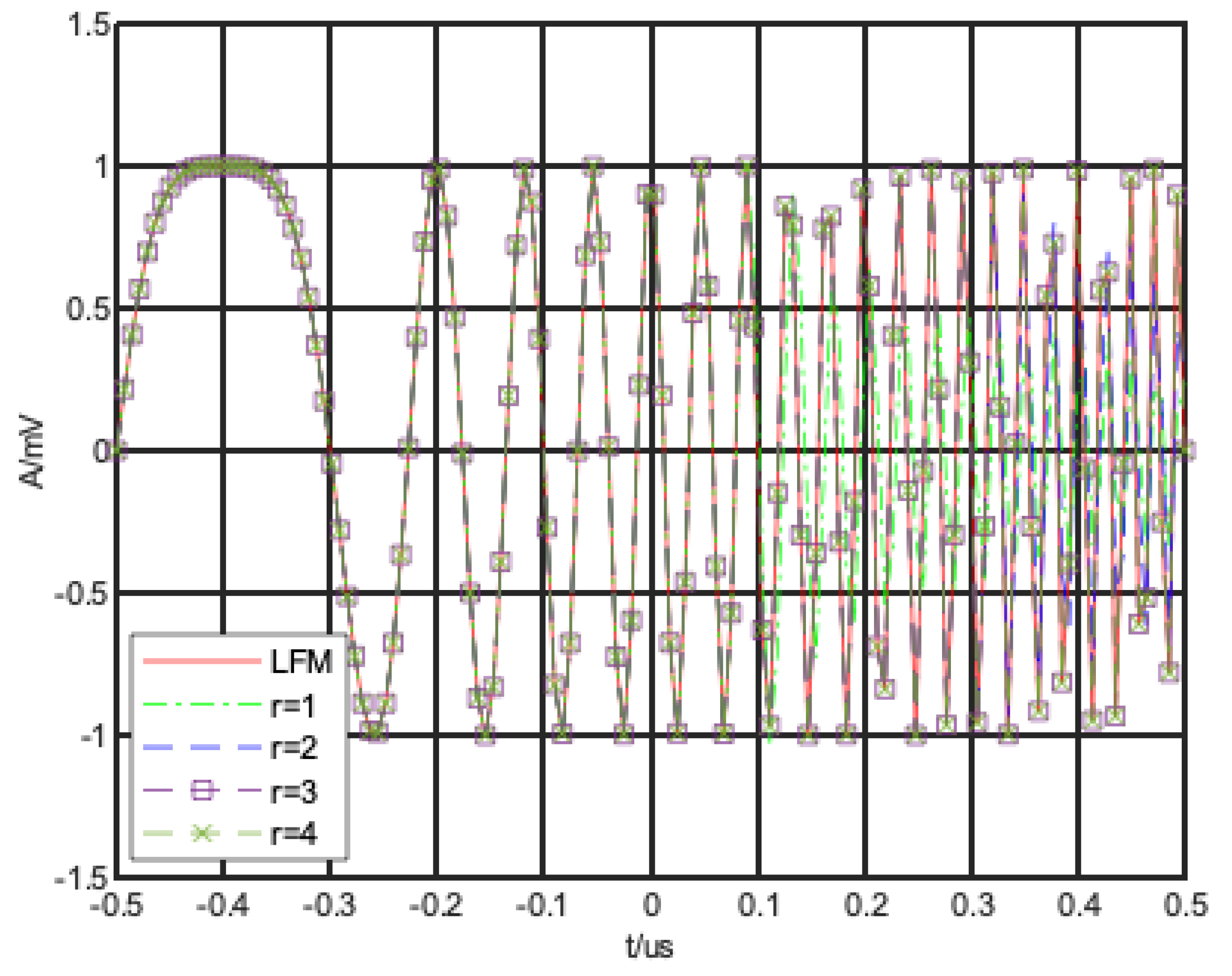
When the parameters for the LFM signal is set to $A=1$, $f_0=20$, $k=50$, the observation time is $T=1$. The signal is sampled according to the Nyquist sampling frequency, and the number of sampling points is $N$ = 140. The tracking factor of the FTD is set to r = 1, 2, 3 and 4. The result is shown in Figure 2.

It can be seen from Figure 2 that in low frequency of the signal, the signal changes slowly. When the tracking factor r = 1~4, FTD can achieve good tracking performance. When the signal is in the mediate frequency, the output signal of FTD with r = 1 still changes with the input signal, but there is phase lag and amplitude reduction. This phenomenon is particularly obvious in high frequency of the signal. In addition, in the case of FTD with r = 2 the phenomenon of “not keeping up” starts to appear when the signal is at high frequency. The FTD with r = 3 and 4 achieves good tracking in the whole frequency band. It can be seen from this that the larger the tracking factor is, the better the tracking performance will be, but the filtering performance will be reduced. Therefore, when designing, the tracking factor should be neither too small nor too large. It should not only ensure that FTD can track signals, but also ensure that it has a certain ability to suppress strong pulses. That is, when encountering strong pulses, there should be a phenomenon similar to “failing to keep up”, such as when r = 1 or 2, as in Figure 2.

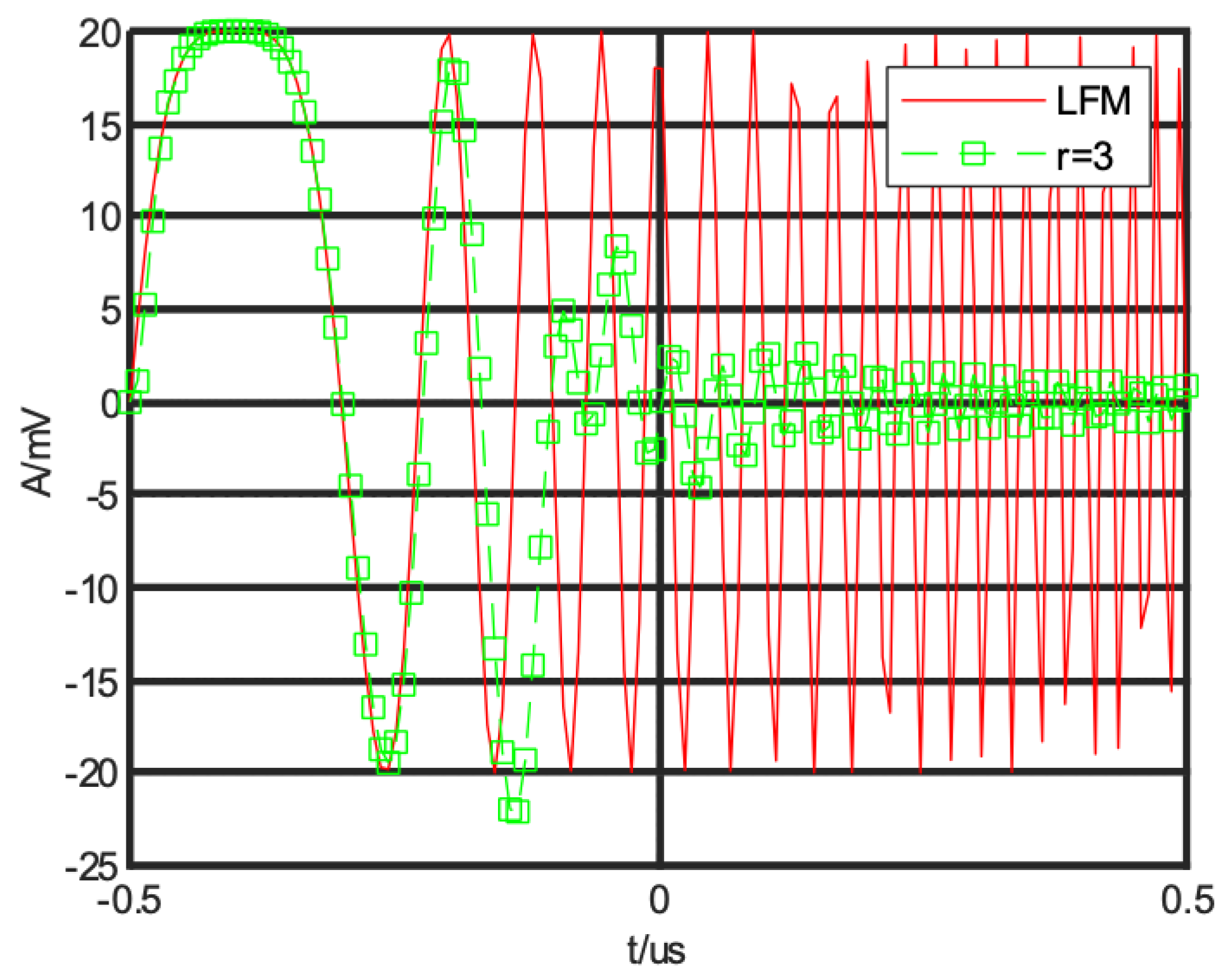
When the parameters for the LFM signal are set as $A=$ 20, $f_0=20$, $k=50$, the observation time is $T=1$. The signal is sampled using the same sampling frequency, and $N$ = 140. The tracking factor of the FTD is set to r = 3. The result is shown in Figure 3.

From the comparison between Figure 2 and Figure 3, it can be seen that the FTD with tracking factor r = 3 can achieve good tracking when the amplitude of the LFM signal is 1. However, when the frequency in unchanged, the tracking performance drops sharply when the amplitude of the signal is 20. It can be seen that the function of the tracking factor of FTD is mainly to adapt to the fluctuation of the adjacent data of the signal. When the signal fluctuation is large, the data is considered to be a strong impulse noise; when the signal fluctuation is small, the data is considered to be a signal or weak noise. FrFT can effectively estimate the parameters of LFM signals in weak impulse noise [19]. Therefore, the main task of FTD is to filter out strong impulse noise. For this reason, we introduce a 3σ criterion to set the tracking factor of FTD.

According to the 3σ criterion, the standard deviation $\sigma (v_0)$ of all echo data $v_0(n)$ in the observation time is calculated, and the initial value is set to 0, that is, $x_1(1)=0$, $x_2(1)=0$. When the difference between the latter data and the former data is greater than $3\sigma (v_0)$, the data are judged to be strong impulse noise, which needs to be suppressed by FTD, so its tracking factor r is set to $3\sigma (v_0)$. This shows that when the change of echo signal does not exceed the value r, the tracking signal changes with the echo signal according to the function $fhan(\cdot )$. When the change of echo signal exceeds the value r, the change of tracking signal is limited to the value r. The proposed FTD is shown in Equation (7), while the $fhan(\cdot )$ is shown in Equation (8).

$$\left\{\begin{array}{c}r=3\sigma (v_0)\\ fh=fhan\left(v_0(n),x_1(n),x_2(n),r\right)\\ x_1(n+1)=x_1(n)+x_2(n)\\ x_2(n+1)=x_2(n)+fh\end{array}\right.$$

(7)

$$\begin{array}{l}fh=-\left\{\begin{array}{c}rsign(a),\left|a\right|>r\\ a,\left|a\right|\le r\end{array}\right.\\ y(n)=x_1(n)-v_0(n)+x_2(n)\\ a_0=\sqrt{r^2+8r|y(n)|}\\ a=\left\{\begin{array}{c}{x}_2(n)+\frac{\left(a_0-r\right)}{2}sign(y(n)),|y(n)|>r\\ x_2(n)+y(n),|y(n)|\le r\end{array}\right.\end{array}$$

(8)

The proposed FTD method in this paper can adaptively set the tracking factor based on the statistical characteristics of the echo data, while the traditional FTD method needs to preset the filter factor. Therefore, the complexity of two algorithms is equivalent, and the proposed FTD method is more flexible and suitable for practical engineering.

3.3. Parameter Estimation Based on FrFT of LFM Signal

The mathematical model for the LFM signal $s(t)$ is shown in Equation (9)

$$s(t)=A\exp (j2\pi (f_{0}t+\frac{1}{2}k{t}^2)), 0\le t\le T,$$

(9)

where $A$, $k$ and $f_0$ denote the amplitude, chirp rate and center frequency of the LFM signal, respectively. $j$ is an imaginary unit and $T$ represents the time-width of the signal $s(t)$.

The $p$-th order continuous FrFT for an LFM signal $s(t)$ can be defined as in Equation (10) [20]

$$X_p(u)=A_{\phi }{\displaystyle \underset{-\infty }{\overset{\infty }{\int }}s(t)\exp [j\pi (u^2+t^2)\cot \phi -j2\pi ut\csc \phi ]}dt,\phi \in (\mathrm{arccot}(\frac{1}{2}),\pi -\mathrm{arccot}(\frac{1}{2})),$$

(10)

where $p$ is the FrFT order, $u$ is the sampling point in the fractional domain, $A_{\phi }=\sqrt{1-j\cot \phi }$, $j$ is an imaginary unit and $\phi =\frac{\pi }{2}p$ represents the rotational angle of the time-frequency plane.

When LFM signals are transformed via the optimal FrFT order, they are converted to impulse signals in the fractional domain. The optimal order $\hat{p}$ and sampling point $\hat{u}$ corresponding the maximum value of ${\left|X_p(u)\right|}^2$ can be searched in the fractional domain:

$$\{\hat{p},\hat{u}\}=\arg \underset{p,u}{\max }{\left|X_p(u)\right|}^2$$

(11)

The optimal FrFT angle can be estimated as

$$\hat{\phi }=\frac{\pi }{2}\hat{p}$$

(12)

The center frequency ${\hat{f}}_0$ and chirp rate $\hat{k}$ of the LFM signal can be calculated as

$${\hat{f}}_0=\hat{u}\csc \hat{\phi },$$

(13)

$$\hat{k}=-\cot \widehat{\phi }.$$

(14)

4. Simulation-Based Experiments and Analysis

4.1. FTD Filtering Performance Verification

Experiment 1: The tracking performance analysis of the two FTDs in noise-free data. The first FTD’s tracking factor is constant; the second FTD’s tracking factor is 3σ of the input data.

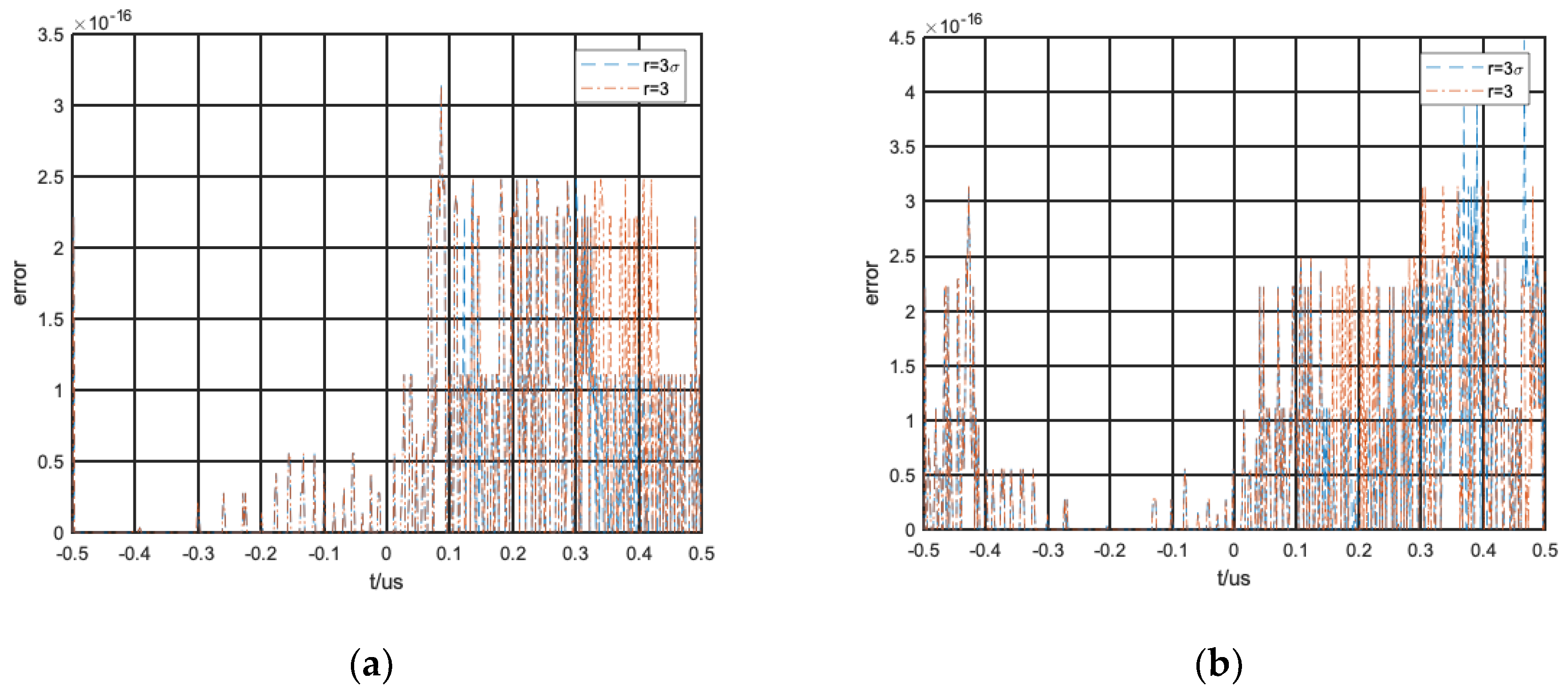
The two sets of input signals are $A=$ 2, $f_0=20$, $k=50$, $T=1$, $N$ = 513 and $A=$ 2, $f_0=20$, $k=100$, $T=1$, $N$ = 1025. The tracking results of these two FTDs is shown in Figure 4 and the tracking error in Figure 5.

It can be seen from Figure 4 that, in order to meet the conditions of FrFT parameter estimation for LFM signals, the sampling frequency must meet the sampling theorem. That is, the number of sampling points must change with the frequency. Under this condition, both FTDs can achieve good tracking. As the tracking error curve shown in Figure 5 demonstrates, their errors are small.

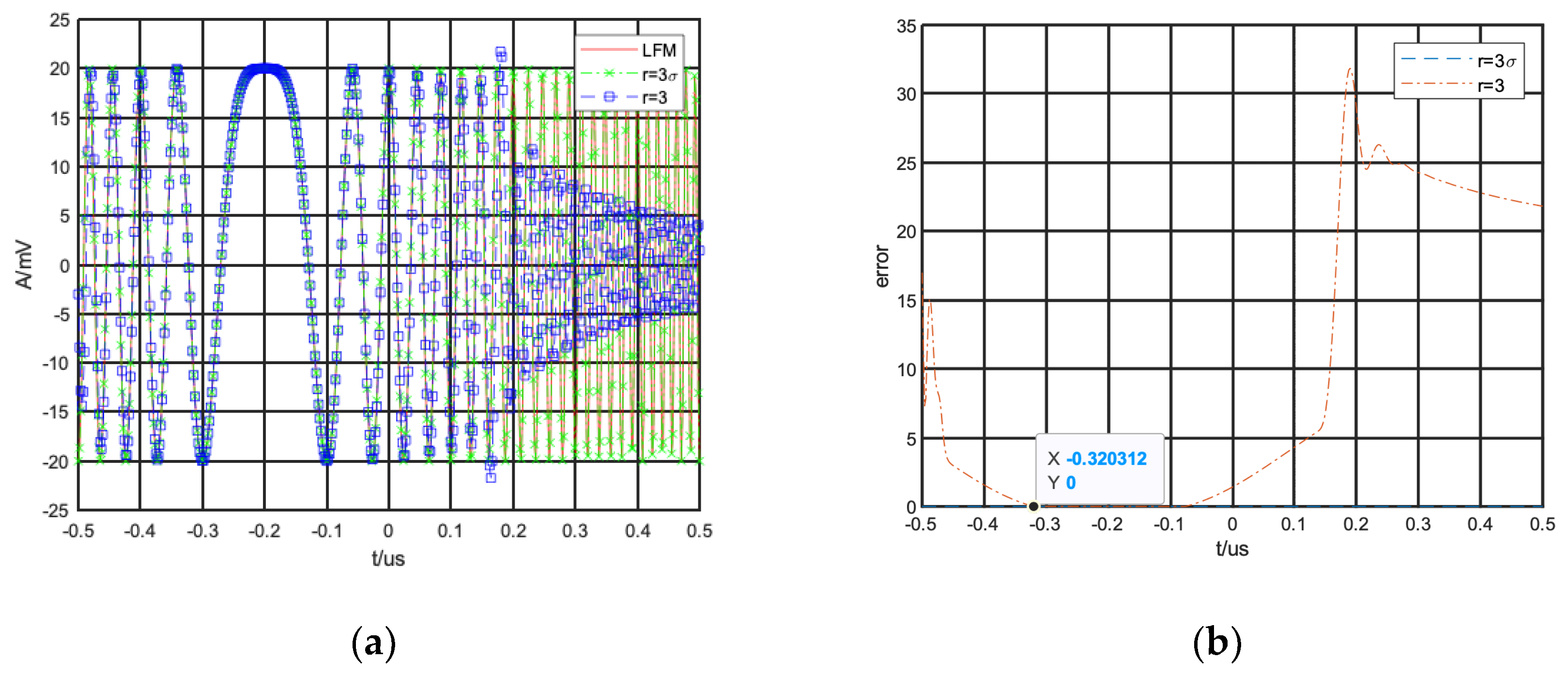
Given the input signal $A=$ 20, $f_0=20$, $k=50$, $T=1$, $N$ = 1025, the results of these two FTDs is shown in Figure 6.

As can be seen from Figure 6a, when the signal amplitude changes and other parameters are unchanged, the tracking factor is set by the 3σ criterion. In such conditions, the FTD can display good tracking performance, while the tracking performance of the fixed value FTD drops sharply in the high-frequency. The tracking error curve is shown in the Figure 6b and, as can be seen, the tracking error of the proposed FTD is still small.

Experiment 2: The filtering performance analysis of the proposed FTD in impulse noise.

The parameters of the LFM signal were set to $A=1$, $f_0=20$, $k=50$. The observation time is $T=1$ and the number of sampling points is $N=513$.

The parameters of alpha stable distribution are $\alpha =$ 2, 1.5, $\beta =0$, $\delta =0.1$, $\mu =0$ and $\alpha =1.5$, $\beta =0$, $\mu =0$, $\delta =0.3$ The filtering results are shown in Figure 7, Figure 8 and Figure 9.

It can be seen from Figure 7 and Figure 8 that when α decreases and the other parameters are unchanged, the impulse characteristics of the noise are enhanced, mainly manifested as an increase in the number of strong impulses, and FTD can effectively realize the tracking performance without showing filtering properties. As the impulse intensity increases, FTD exhibits a suppressive effect on the impulse noise, as shown in Figure 8.

It can be seen from Figure 8 and Figure 9 that when δ increases and the other parameters are unchanged, the impulse characteristics of the noise are also enhanced, mainly due to the increase of noise intensity and of the number of impulses. Still, FTD shows a good suppression effect against strong impulse noise.

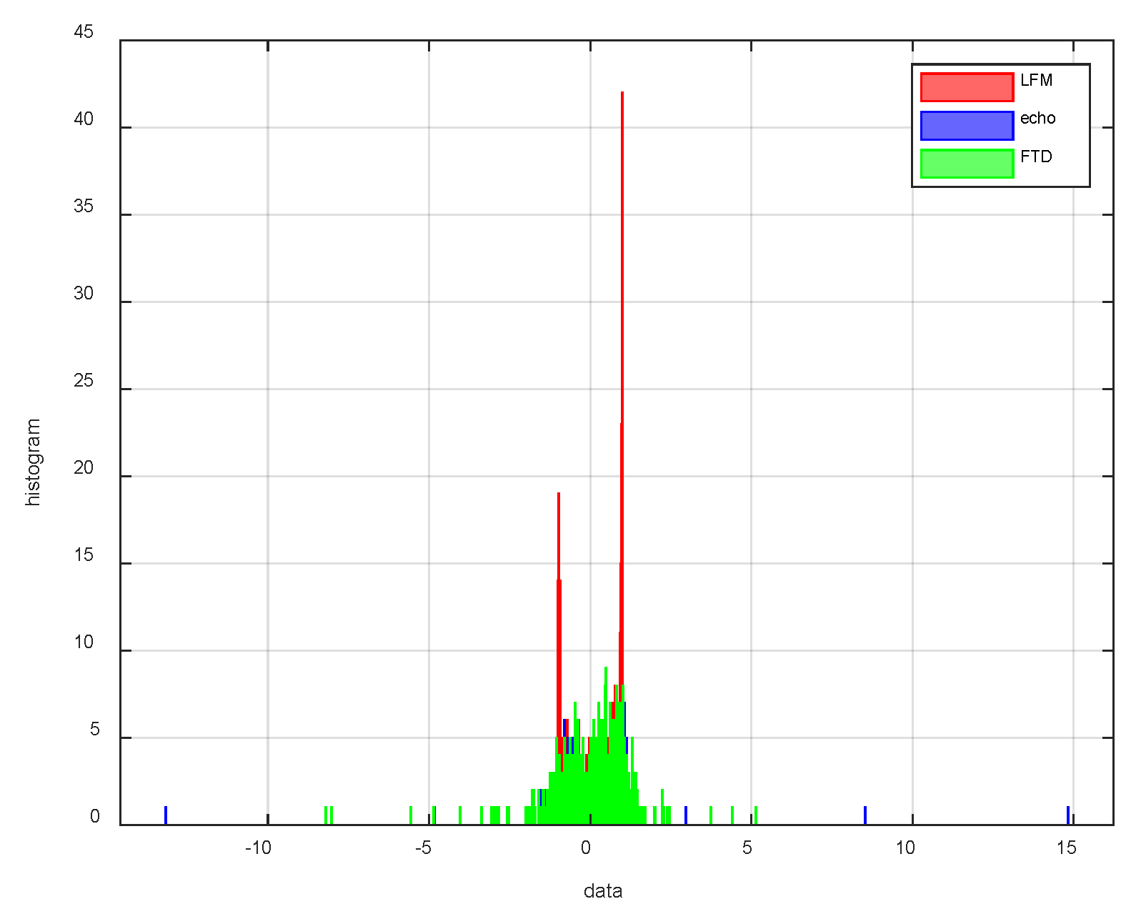
Figure 10 is the histogram of the three data in Figure 9, where the red square stands for the statistics of noise-free data, the blue square is the statistics of noisy data, and the green square is the statistics of the echo signal processed by FTD. It can clearly be seen from Figure 10 that the red data are concentrated in the [−1,1], that the blue data have some strong impulse data, and that the strong impulse is suppressed by FTD in the green data. Lastly, there is a trend of aggregation in the direction of the data mean.

From these experiments, it can be seen that the proposed FTD can effectively suppress strong impulse noise.

4.2. Verification of LFM Signal Parameter Estimation Accuracy

The parameters for an LFM signal were set to $A=1$, $f_0=20$, $k=50$, $T=1$, $N=513$.

Experiment 1: The parameter estimation performance analysis of the proposed FTD-FrFT in impulse noise.

Adding the impulse noise of alpha stable distribution with different parameters to the LFM signal, the parameters of the alpha stable distribution are $\alpha =2~0.1$, $\beta =0$, $\delta =0.1$, $\mu =0$, $\alpha =1.5$, $\beta =-1~1$, $\delta =0.1$, $\mu =0$, $\alpha =1.5$, $\beta =0$, $\delta =0.1~1$, $\mu =0$ and $\alpha =1.5$, $\beta =0$, $\delta =0.1$, $\mu =-1~1$.

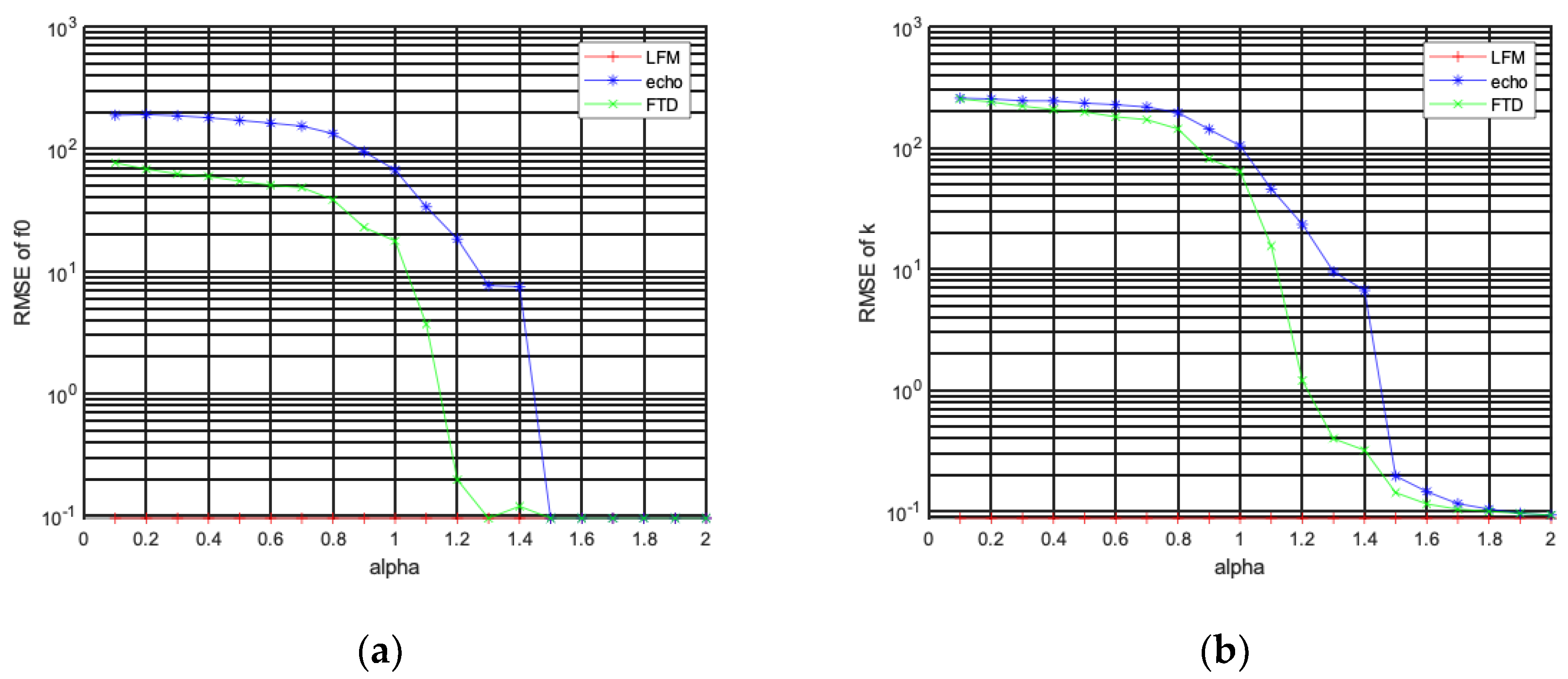
FrFT was used to estimate the parameters of the LFM signal, echo signal and the FTD filtered signal, respectively. We performed 1000 Monte Carlo trial runs and calculated the root mean square error for the estimated central frequency and chirp rate of thee LFM signal. The simulation results are presented in Figure 11.

It can be seen from Figure 11 that when α ≥ 1.5, the FrFT method can be used to effectively estimate the LFM signal parameters, but when α is less than 1.5, the FrFT method affected by impulse noise begins to fail. The proposed FTD-FrFT method effectively estimates the parameters of LFM signals when α is greater than or equal to 1.2, and the estimation error is lower than that of the FrFT parameter estimation method. The estimation accuracy can even be close to that of noise-free LFM signal parameter estimation accuracy when the impulse noise is small.

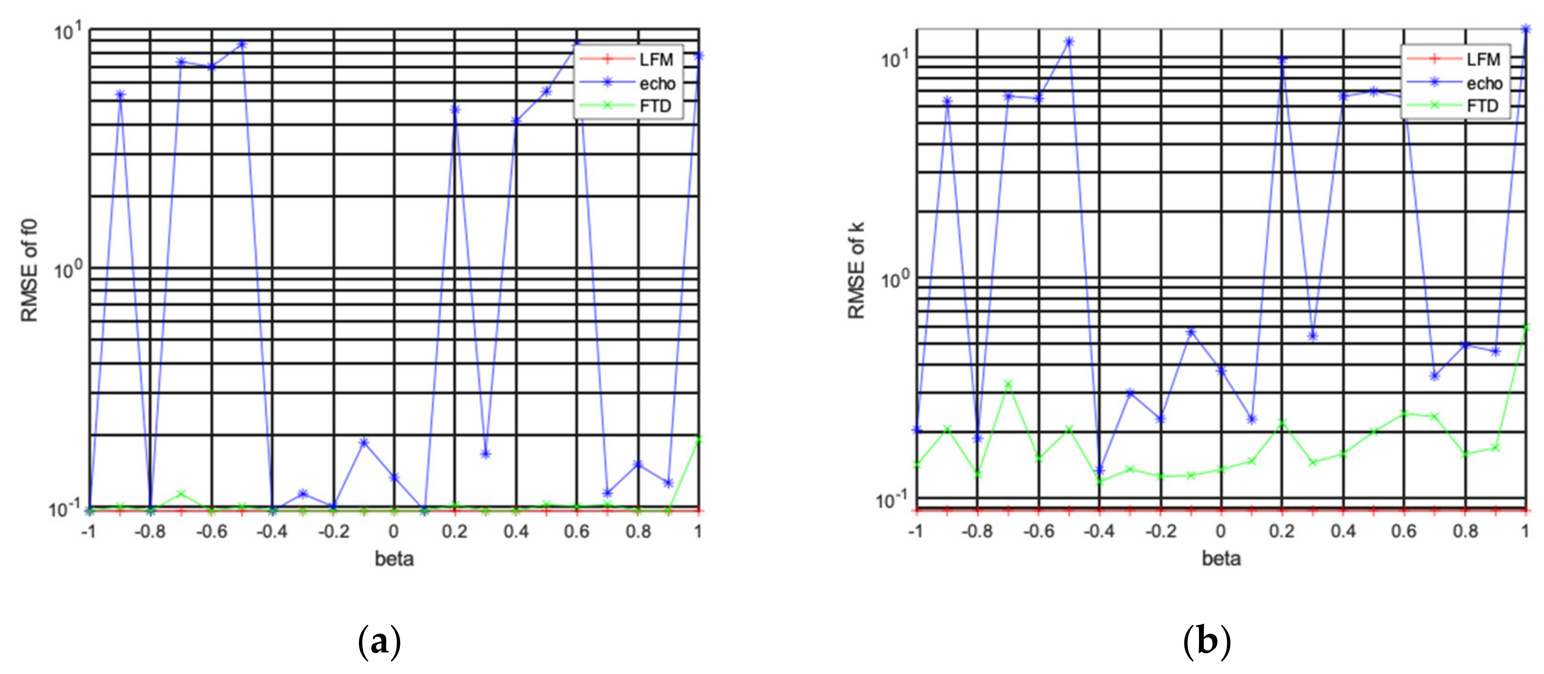
As can be seen from Figure 12, the performance of the FrFT parameter estimation method is unstable in different β, and the proposed FTD-FrFT method still shows a better parameter estimation performance when the parameter β changes. This shows that the proposed method can not only effectively suppress impulse noise, but also adapt to the impulse noise of a non-zero mean.

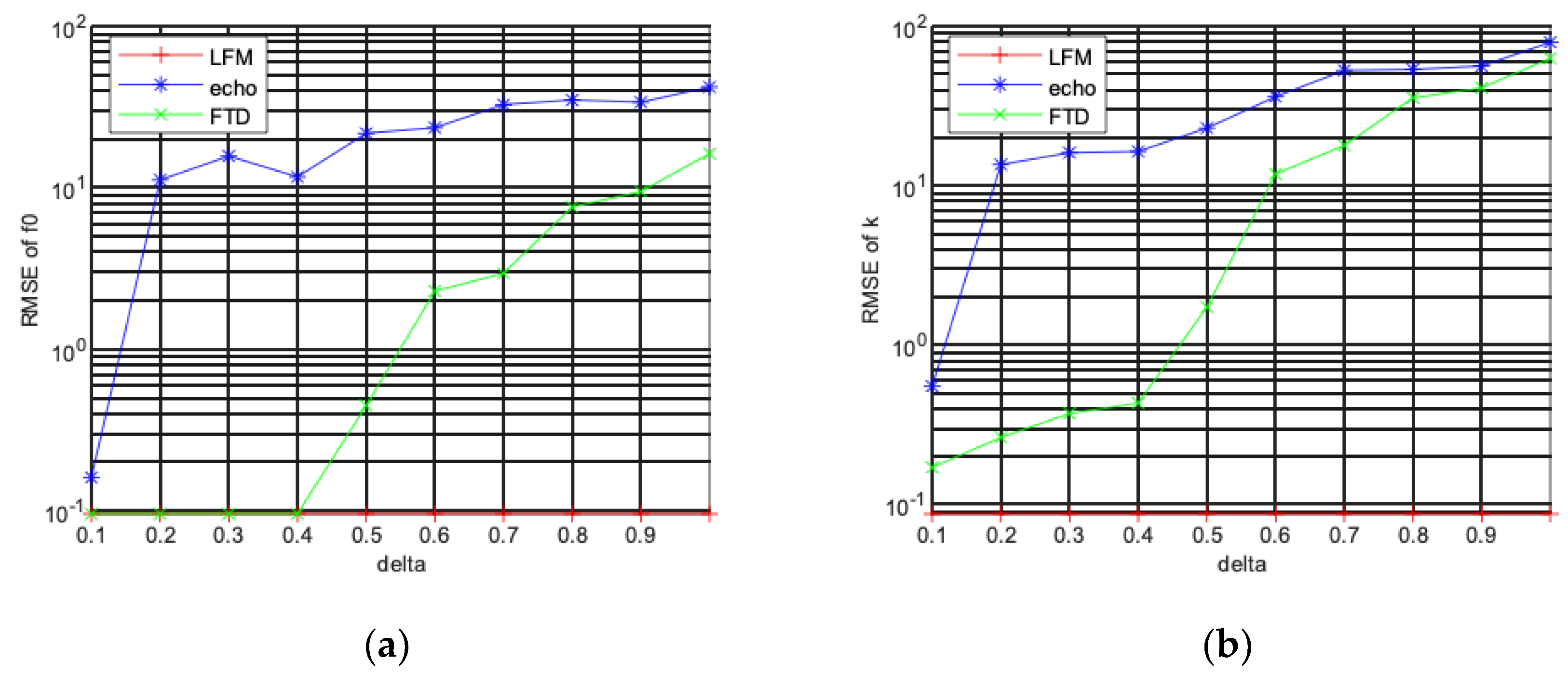
As can be seen from Figure 13, when δ ≥ 0.2, the FrFT parameter estimation method is affected by the impulse noise and begins to fail. However, the proposed FTD-FrFT method only begins to fail at δ > 0.4, and the estimation error is lower than that of the FrFT parameter estimation method.

As can be seen from Figure 14, the performance of the FrFT parameter estimation method is unstable in different μ. However, the proposed FTD-FrFT method shows a better parameter estimation performance from −0.6 to 0.6. As can be seen, this method can not only effectively suppress impulse noise, but also adapt to non-zero mean impulse noise.

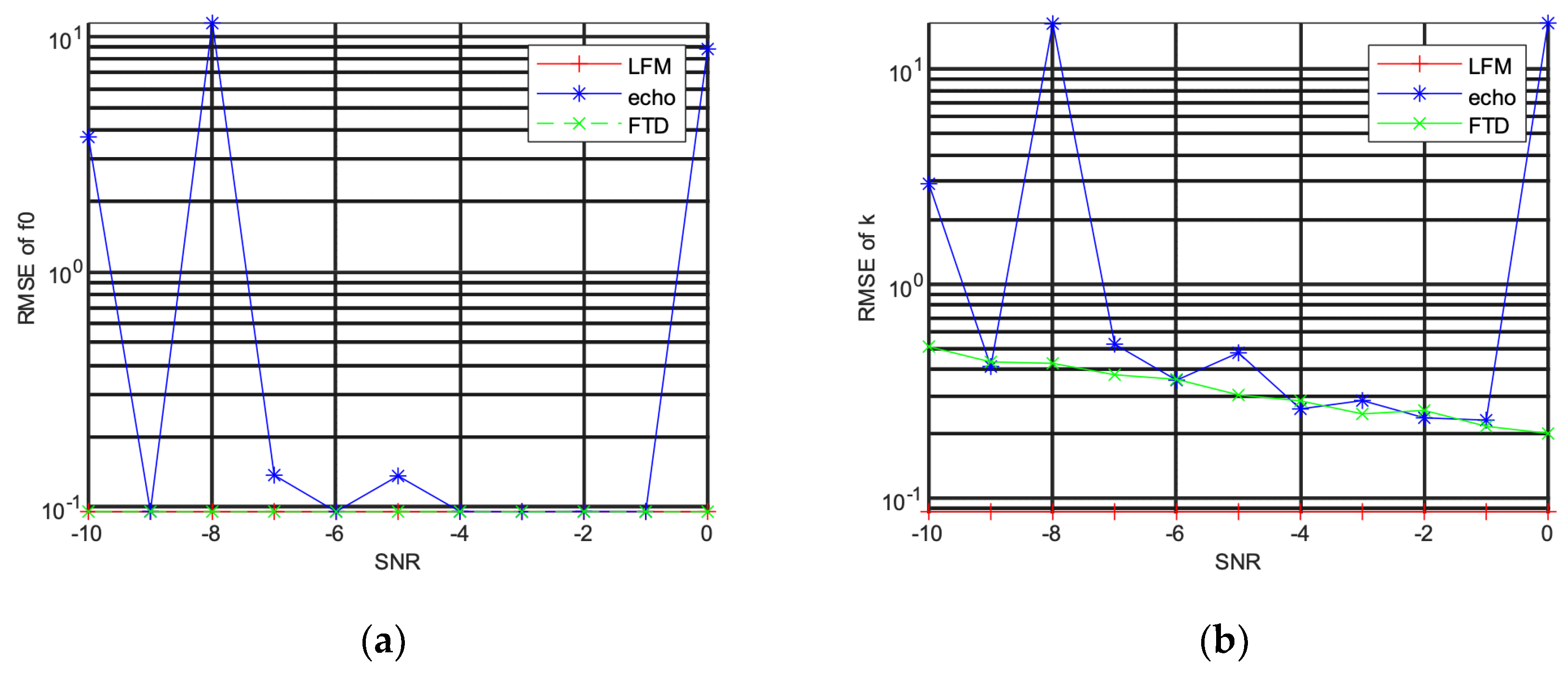
Experiment 3: We compared the performance of these parameter estimation methods for an LFM signal with mixed noise.

Adding the mixed noise of Gaussian noise and α noise to an LFM signal, the Gaussian noise signal-to-noise ratio is 0~−10 dB, and the parameters of the α noise are $\alpha =1.5$, $\beta =0$, $\delta =0.1$, $\mu =0$. FrFT was used to estimate the parameters of the LFM signal, echo signal and the signal filtered by the FTD. We performed 500 Monte Carlo trial runs. The center frequency and chirp rate of the LFM signal are estimated, and the simulation results are presented in Figure 15.

As can be seen from Figure 15, the FrFT parameter estimation method is affected by mixed noise. This causes the parameter estimation performance to be unstable, while the proposed FTD-FrFT method still displays a reliable parameter estimation performance in mixed noise.

5. Conclusions

This paper proposes a new parameter estimation method for LFM signals that combines FTD and FrFT. The proposed technique is based on the basic FTD, with the addition of an adaptive tracking factor of FTD to better suppress impulse noise and make FrFT methods better estimate LFM signal parameters. The results of a series of simulations demonstrate that the proposed method can effectively suppress the impulse noise with different parameters. The parameter estimation accuracy of the FTD-FrFT method is higher than that of the FrFT method, and the estimation performance in the mixed noise is more stable than that of the FrFT method. Overall, the proposed FTD-FrFT method exhibits a high estimation accuracy in impulse noise.

References

1. Dong, N.; Wang, J. Sub-Nyquist sampling and parameters estimation of wideband Chirp signals based on FRFT. Radioelectron. Commun. Syst. 2018, 61, 333–341. [Google Scholar] [CrossRef]
2. Guo, L.-B.; Tang, J.-L.; Dong, Y.-Y.; Dong, C.-X. One-bit LFM signal recovery via random threshold strategy. Digit. Signal Process. 2021, 111, 102965. [Google Scholar] [CrossRef]
3. Guo, Q.; Zhang, F.; Zhou, P.; Pan, S. Dual-Band LFM Signal Generation by Optical Frequency Quadrupling and Polarization Multiplexing. IEEE Photon-Technol. Lett. 2017, 29, 1320–1323. [Google Scholar] [CrossRef]
4. Ji, J.; Zheng, S.; Zhang, X. Pre-distortion compensation for optical-based broadband LFM signal generation system. Opt. Commun. 2019, 435, 277–282. [Google Scholar] [CrossRef]
5. Jiang, L.; Li, L.; Zhao, G.; Pan, Y. Instantaneous Frequency Estimation of Nonlinear Frequency-Modulated Signals Under Strong Noise Environment. Circuits Syst. Signal Process. 2016, 35, 3734–3744. [Google Scholar] [CrossRef]
6. Liu, X.; Xiao, B.; Wang, C. Frequency estimation of chirp signals based on fractional fourier transform combined with Otsu’s method. Optik 2021, 240, 166945. [Google Scholar] [CrossRef]
7. Liu, X.; Han, J.; Wang, C.; Xiao, B. Parameters Estimation for Chirp Signal Based on QPF-FRFT. Optik 2019, 182, 529–537. [Google Scholar] [CrossRef]
8. Miao, H.; Zhang, F.; Tao, R. Mutual Information Rate of Nonstationary Statistical Signals. Signal Process. 2020, 171, 107531. [Google Scholar] [CrossRef]
9. Moghadasian, S.S.; Gazor, S. Sparsely Localized Time-Frequency Energy Distributions for Multi-Component LFM Signals. IEEE Signal Process. Lett. 2020, 27, 6–10. [Google Scholar] [CrossRef]
10. Stuck, W.; Kleiner, B. A statistical analysis of telephone noise. Bell Syst. Tech. J. 1974, 53, 1263–1320. [Google Scholar] [CrossRef]
11. Nikias, C.L.; Shao, M. Signal Processing with Alpha-Stable Distributions and Applications; Wiley: New York, NY, USA, 1995. [Google Scholar]
12. Engin, K.E. Signal Processing with Fractional Lower Order Environments at Least lp-Norm Approach. Ph.D. Thesis, University of Cambridge, London, UK, 1998. [Google Scholar]
13. Yang, F.; Jia, H.; Liu, B.; Long, K. Performance analysis of broadband power-line communications systems under the alpha-stable impulsive noise. J. Electron. Inf. Technol. 2019, 41, 1374–1380. [Google Scholar] [CrossRef]
14. Gu, G.-D.; Zhang, Y.-S.; Tian, B. Estimation of LFM signal’s time parameters under the alpha-stable distribution noise. In Proceedings of the IEEE Circuits and Systems International Conference on Testing and Diagnosis, Chengdu, China, 28 April 2009; pp. 1–4. [Google Scholar]
15. Jin, Y.; Duan, P.T.; Ji, H.B. Parameter estimation of LFM Signals based on LVD in complicated noise environments. J. Electron. Inform. Technol. 2014, 36, 1106–1112. [Google Scholar]
16. Liu, X.; Wang, C. A Novel Parameter Estimation of Chirp Signal in α-Stable Noise. IEICE Electron. Express 2017, 14, 20161053. [Google Scholar] [CrossRef] [Green Version]
17. Zhang, H.; Xiao, G.; Yu, X.; Xie, Y. On Convergence Performance of Discrete-Time Optimal Control Based Tracking Differentiator. IEEE Trans. Ind. Electron. 2020, 68, 3359–3369. [Google Scholar] [CrossRef]
18. Wang, Z.; Long, Z.; Xie, Y.; Ding, J.; Luo, J.; Li, X. A Discrete Nonlinear Tracking-Differentiator and Its Application in Vibration Suppression of Maglev System. Math. Probl. Eng. 2020, 2020 Pt 20, 1849816.1–1849816.9. [Google Scholar] [CrossRef]
19. Liu, X.; Xiao, B.; Wang, C. Optimal Target Function for the Fractional Fourier Transform of LFM Signals. Circuits Syst. Signal Process. 2022, 41, 4160–4173. [Google Scholar] [CrossRef]
20. Liu, X.; Han, J.; Wang, C.; Xiao, B. Parameter estimation of linear frequency modulation signals based on sampling theorem and fractional broadening. Rev. Sci. Instrum. 2019, 90, 014702. [Google Scholar] [CrossRef] [PubMed]
Figure 1. The probability density functions of alpha stable distribution with different parameters. (a) different α ; (b) different β ; (c) different δ ; (d) different μ .
Fractalfract 07 00069 g001
Figure 2. The result of FTD with the different tracking factors.
Fractalfract 07 00069 g002
Figure 3. The result of FTD with tracking factor r = 3.
Fractalfract 07 00069 g003
Figure 4. The tracking results of these two FTDs: (a) The first input signal; (b) The second input signal.
Fractalfract 07 00069 g004
Figure 5. The error results of these two FTDs: (a) The error for the first input signal; (b) The error for the second input signal.
Fractalfract 07 00069 g005
Figure 6. The compared results of these two FTDs: (a) The tracking of input signal; (b) The error of input signal.
Fractalfract 07 00069 g006
Figure 7. Filtering results with α = 2 , β = 0 ,   δ = 0.1 ,   μ = 0 .
Fractalfract 07 00069 g007
Figure 8. Filtering results with α = 1 , β = 0 ,   δ = 0.1 ,   μ = 0 .
Fractalfract 07 00069 g008
Figure 9. Filtering results with α = 1.5 , β = 0 ,   δ = 0.3 ,   μ = 0 .
Fractalfract 07 00069 g009
Figure 10. Histogram of three data in Figure 9.
Fractalfract 07 00069 g010
Figure 11. RMSE of parameter estimation with α = 2 ~ 0.1 , β = 0   , δ = 0.1   , μ = 0 : (a) RMSE of f0; (b) RMSE of k.
Fractalfract 07 00069 g011
Figure 12. RMSE of parameter estimation with α = 1.5 , β = 1 ~ 1 , δ = 0.1   , μ = 0 : (a) RMSE of f0; (b) RMSE of k.
Fractalfract 07 00069 g012
Figure 13. RMSE of parameter estimation with α = 1.5 , β = 0   , δ = 0.1 ~ 1   , μ = 0 : (a) RMSE of f0; (b) RMSE of k.
Fractalfract 07 00069 g013
Figure 14. RMSE of parameter estimation with α = 1.5 , β = 0   , δ = 0.1 , μ = 1 ~ 1 : (a) RMSE of f0; (b) RMSE of k.
Fractalfract 07 00069 g014
Figure 15. RMSE of parameter estimation with mixed noise: (a) RMSE of f0; (b) RMSE of k.
Fractalfract 07 00069 g015
Disclaimer/Publisher’s Note: The statements, opinions and data contained in all publications are solely those of the individual author(s) and contributor(s) and not of MDPI and/or the editor(s). MDPI and/or the editor(s) disclaim responsibility for any injury to people or property resulting from any ideas, methods, instructions or products referred to in the content.