Approximation Theorems Associated with Multidimensional Fractional Fourier Transform and Applications in Laplace and Heat Equations

Abstract

In this paper, we establish two approximation theorems for the multidimensional fractional Fourier transform via appropriate convolutions. As applications, we study the boundary and initial problems of the Laplace and heat equations with chirp functions. Furthermore, we obtain the general Heisenberg inequality with respect to the multidimensional fractional Fourier transform.

1. Introduction

The classical Fourier transform (FT) is one of the most influential tools in signal processing. With the development of signal processing theory, some researchers realized that the fractional Fourier transform (FRFT) is well suited to processing complicated signals. It can reflect the information of signals in both the time domain and the frequency domain. Therefore, it can deal with time-varying degradation models and non-stationary processes. In recent decades, the FRFT has become an attractive tool and has various applications in many fields of applied sciences, such as signal processing [1,2], image processing [3,4,5], optics [6,7,8], communications [9,10,11], quantum mechanics [12,13] and so on.

Wiener first introduced the FRFT in his 1929 work [14]. Namias proposed the FRFT in [12] using its eigenvalue equation. Since Namias’ work in 1980, the FRFT has attracted a lot of interest. Compared with FT, the FRFT contains one extra free parameter and is more suited to process non-stationary signals, especially chirp signals. As a result, FRFT can achieve effects that the classical Fourier transform or time-frequency analysis cannot.

Recall that for appropriate function $f\in {\mathbb{R}}^n$, the nd-FT of f is defined by (see [15])

$$\mathcal{F}f\left(\mathit{u}\right)=\begin{array}{c}{\displaystyle {\int }_{{\mathbb{R}}^n}f\left(\mathit{x}\right)e^{-2\pi i\mathit{x}·\mathit{u}}\mathrm{d}\mathit{x}.}\hfill \end{array}$$

For $f\in L^1\left({\mathbb{R}}^n\right)$ and $\mathit{\alpha }=({\alpha }_1,{\alpha }_2,\dots ,{\alpha }_n)\in {\mathbb{R}}^n$, the nd-FRFT of f with order $\mathit{\alpha }$ is defined by (see [16,17])

$$\begin{array}{c}\hfill {\mathcal{F}}_{\mathit{\alpha }}f\left(\mathit{z}\right)={\int }_{{\mathbb{R}}^n}{K}_{\mathit{\alpha }}(\mathit{x},\mathit{z})f\left(\mathit{x}\right)\mathrm{d}\mathit{x},\end{array}$$

(1)

where $K_{\mathit{\alpha }}(\mathit{x},\mathit{z})={\prod }_{j=1}^n{K}_{{\alpha }_j}(x_j,z_j)$ and here for each $j=1,2,\cdots ,n$, $K_{{\alpha }_j}(x_j,z_j)$ is defined as follows

$$\begin{array}{c}\hfill K_{{\alpha }_j}(x_j,z_j)=\left\{\begin{array}{cc}\sqrt{1-i\cot {\alpha }_j}{e}^{i\pi \cot {\alpha }_j[x_j^2+z_j^2-2x_j{z}_j\sec {\alpha }_j]},\hfill & {\alpha }_j\notin \pi \mathbb{Z},\hfill \\ \\ \delta (x_j-z_j),\hfill & {\alpha }_j\in 2\pi \mathbb{Z},\hfill \\ \\ \delta (x_j+z_j),\hfill & {\alpha }_j\in 2\pi \mathbb{Z}+\pi ,\hfill \end{array}\right.\end{array}$$

(2)

where $\mathit{x}=(x_1,x_2,\cdots ,x_n)$.

Throughout this paper, we fix $\mathit{\alpha }\in {\mathbb{R}}^n$ with ${\alpha }_j\ne k\pi$, $j=1,2,\dots ,n$. Then,

$$\begin{array}{c}\hfill K_{\mathit{\alpha }}(\mathit{x},\mathit{z})=A_{\mathit{\alpha }}{e}_{\mathit{\alpha }}\left(\mathit{z}\right)e_{\mathit{\alpha }}\left(\mathit{x}\right)e_{\mathit{\alpha }}(\mathit{x},\mathit{z}),\end{array}$$

(3)

where

$$\begin{array}{c}\hfill \left\{\begin{array}{c}{A}_{\mathit{\alpha }}={\displaystyle \prod _{j=1}^n}{A}_{{\alpha }_j}={\displaystyle \prod _{j=1}^n}\sqrt{1-i\cot {\alpha }_j},\hfill \\ \\ e_{\mathit{\alpha }}\left(\mathit{x}\right)={\displaystyle \prod _{j=1}^n}{e}_{{\alpha }_j}\left(x_j\right)=e^{i\pi {\displaystyle \sum _{j=1}^n}{x}_j^2\cot {\alpha }_j},\hfill \\ \\ e_{\mathit{\alpha }}(\mathit{x},\mathit{z})={\displaystyle \prod _{j=1}^n}{e}_{{\alpha }_j}(x_j,z_j)=e^{-2i\pi {\displaystyle \sum _{j=1}^n}{z}_j{x}_j\csc {\alpha }_j}.\hfill \end{array}\right.\end{array}$$

(4)

It is obvious that

$$\begin{array}{c}\hfill \left({\mathcal{F}}_{\mathit{\alpha }}f\right)\left(\mathit{z}\right)=A_{\mathit{\alpha }}{e}_{\mathit{\alpha }}\left(\mathit{z}\right)\mathcal{F}\left(e_{\mathit{\alpha }}f\right)\left({\mathit{z}}_{\mathit{\alpha }}\right)\end{array}$$

(5)

where ${\mathit{z}}_{\mathit{\alpha }}=(z_1\csc {\alpha }_1,z_2\csc {\alpha }_2\dots ,z_n\csc {\alpha }_n)$.

For the 1-dimensional case, Chen et al. [18] studied the approximation theorem for FRFT. A new 2d-FRFT was proposed by Zayed in [19], where the convolution theorem and Poisson summation formula were proved. It is natural for us to investigate cases in high dimensions. By combining the definitions provided by [18,20,21], the multidimensional fractional convolution of order $\mathit{\alpha }$ can be defined as follows. For $f,g\in L^1\left({\mathbb{R}}^n\right)$,

$$\begin{array}{c}\hfill \left(f\stackrel{\mathit{\alpha }}{\ast }g\right)\left(\mathit{x}\right)=e_{-\mathit{\alpha }}\left(\mathit{x}\right){\int }_{{\mathbb{R}}^n}{e}_{\mathit{\alpha }}\left(\mathit{z}\right)f\left(\mathit{z}\right)g(\mathit{x}-\mathit{z})\mathrm{d}\mathit{z}.\end{array}$$

(6)

We establish the following two approximation theorems, where Theorem 1 is approximation in $L^p$ norm and Theorem 2 is almost everywhere approximation.

Theorem 1.

Let $\varphi \in L^1\left({\mathbb{R}}^n\right)$, $f\in L^p\left({\mathbb{R}}^n\right),1\le p<\infty$ and ${\int }_{{\mathbb{R}}^n}\varphi \left(\mathit{x}\right)\mathrm{d}\mathit{x}=1$. Then

$$\begin{array}{c}\hfill \underset{y\to 0}{lim}{∥\left(f\stackrel{\mathit{\alpha }}{\ast }{\varphi }_y\right)-f∥}_p=0\end{array}$$

(7)

where ${\varphi }_y:=\frac{1}{y^n}\varphi \left(\frac{·}{y}\right)$.

Theorem 2.

Let $\varphi \in L^1\left({\mathbb{R}}^n\right)$, $f\in L^p\left({\mathbb{R}}^n\right),1\le p<\infty$ and ${\int }_{{\mathbb{R}}^n}\varphi \left(\mathit{x}\right)\mathrm{d}\mathit{x}=1$. Denote by $\psi \left(\mathit{z}\right)={sup}_{\left|\mathit{x}\right|\ge \mathit{z}}\left|\varphi \left(\mathit{x}\right)\right|$ the decreasing radial dominant function of ϕ. If $\psi \in L^1\left({\mathbb{R}}^n\right)$, then for almost all $\mathit{z}\in {\mathbb{R}}^n$,

$$\begin{array}{c}\hfill \underset{y\to 0}{lim}\left(f\stackrel{\mathit{\alpha }}{\ast }{\varphi }_y\right)\left(\mathit{z}\right)=f\left(\mathit{z}\right),\end{array}$$

(8)

where ${\varphi }_y:=\frac{1}{y^n}\varphi \left(\frac{·}{y}\right)$.

The uncertainty principle is a principle of physics introduced by Heisenberg in 1927. It points out that it is impossible to precisely determine the position and momentum of a microscopic particle at the same time. It is one of the fundamental results in quantum mechanics. The uncertainty principle is expressed mathematically as the Heisenberg inequality. In this paper, we study the general Heisenberg inequality.

Theorem 3

(General Heisenberg inequality). Let $f\in L^2\left({\mathbb{R}}^n\right)$ and $\mathit{\alpha }=({\alpha }_1,{\alpha }_2,\dots ,{\alpha }_n)$, $\mathit{\beta }=({\beta }_1,{\beta }_2,\dots ,{\beta }_n)\in {\mathbb{R}}^n.$ For any $\mathit{y}=(y_1,y_2,\dots ,y_n),\mathit{v}=(v_1,v_2,\dots ,v_n)\in {\mathbb{R}}^n$, if ${\alpha }_1-{\beta }_1={\alpha }_2-{\beta }_2=\dots ={\alpha }_n-{\beta }_n$, then

$$\begin{array}{cc}\hfill & \left[{\int }_{{\mathbb{R}}^n}{\left|\mathit{x}-\tilde{\mathit{y}}\right|}^2{\left|\left({\mathcal{F}}_{\mathit{\alpha }}f\right)\left(\mathit{x}\right)\right|}^2\mathrm{d}\mathit{x}\right]\left[{\int }_{{\mathbb{R}}^n}{\left|\mathit{z}-\tilde{\mathit{v}}\right|}^2{\left|\left({\mathcal{F}}_{\mathit{\beta }}f\right)\left(\mathit{z}\right)\right|}^2\mathrm{d}\mathit{z}\right]\ge \frac{n^2{\parallel f\parallel }_2^4}{16{\pi }^2}{\sin }^2({\alpha }_1-{\beta }_1),\hfill \end{array}$$

(9)

where

$$\tilde{\mathit{y}}=\left(y_1\sin {\alpha }_1+v_1\cos {\alpha }_1,y_2\sin {\alpha }_2+v_2\cos {\alpha }_2,\dots ,y_n\sin {\alpha }_n+v_n\cos {\alpha }_n\right),$$

$$\tilde{\mathit{v}}=\left(y_1\sin {\beta }_1+v_1\cos {\beta }_1,y_2\sin {\beta }_2+v_2\cos {\beta }_2,\dots ,y_n\sin {\beta }_n+v_n\cos {\beta }_n\right).$$

In Section 2, we prove the above theorems. As applications, we investigate the Laplace and heat equations with boundary and initial conditions for chirp functions in Section 3. Furthermore, we demonstrate the effectiveness of our method through graphs in Section 4.

2. The Proof of Theorems

Firstly, we prove two approximation theorems. Before proving Theorem 1, we need the following lemma.

Lemma 1.

Let $f\in L^p\left({\mathbb{R}}^n\right),1\le p<\infty$. Then, for every $\mathit{x}\in {\mathbb{R}}^n$

$$\begin{array}{c}\hfill \underset{y\to 0}{lim}{\left\{{\int }_{{\mathbb{R}}^n}{\left|e^{{\displaystyle \sum _{j=1}^n}i\pi \cot {\alpha }_j\left[{\left(z_j-y{x}_j\right)}^2-z_j^2\right]}f\left(\mathit{z}-y\mathit{x}\right)-f\left(\mathit{z}\right)\right|}^p\mathrm{d}\mathit{z}\right\}}^{\frac{1}{p}}=0.\end{array}$$

(10)

Proof. 

Since the space of continuous functions with compact support $C_c\left({\mathbb{R}}^n\right)$ is dense in $L^p\left({\mathbb{R}}^n\right)$, for an arbitrary $\epsilon >0$, there exists $g\in C_c\left({\mathbb{R}}^n\right)$, satisfying

$${∥f-g∥}_p<\frac{\epsilon }{2}.$$

Because g is uniformly continuous, we have

$$\begin{array}{c}\hfill \underset{y\to 0}{lim}\left|g\left(\mathit{z}-y\mathit{x}\right)-g\left(\mathit{z}\right)\right|=0.\end{array}$$

(11)

We can write

$$\begin{array}{cc}\hfill J_y\left(x\right):=& {\left\{{\int }_{{\mathbb{R}}^n}{\left|e^{{\displaystyle \sum _{j=1}^n}i\pi \cot {\alpha }_j\left[{\left(z_j-y{x}_j\right)}^2-z_j^2\right]}f\left(\mathit{z}-y\mathit{x}\right)-f\left(\mathit{z}\right)\right|}^p\mathrm{d}\mathit{z}\right\}}^{\frac{1}{p}}\hfill \\ \hfill \le & {\left\{{\int }_{{\mathbb{R}}^n}{\left|e^{{\displaystyle \sum _{j=1}^n}i\pi \cot {\alpha }_j\left[{\left(z_j-y{x}_j\right)}^2-z_j^2\right]}\left[f\left(\mathit{z}-y\mathit{x}\right)-g\left(\mathit{z}-y\mathit{x}\right)\right]\right|}^p\mathrm{d}\mathit{z}\right\}}^{\frac{1}{p}}\hfill \\ \hfill & +{\left\{{\int }_{{\mathbb{R}}^n}{\left|e^{{\displaystyle \sum _{j=1}^n}i\pi \cot {\alpha }_j\left[{\left(z_j-y{x}_j\right)}^2-z_j^2\right]}g\left(\mathit{z}-y\mathit{x}\right)-g\left(\mathit{z}-y\mathit{x}\right)\right|}^p\mathrm{d}\mathit{z}\right\}}^{\frac{1}{p}}\hfill \\ \hfill & +{\left\{{\int }_{{\mathbb{R}}^n}{\left|g\left(\mathit{z}-y\mathit{x}\right)-g\left(\mathit{z}\right)\right|}^p\mathrm{d}\mathit{z}\right\}}^{\frac{1}{p}}+{∥f-g∥}_p\hfill \\ \hfill \le & 2{∥f-g∥}_p+{∥g∥}_{\infty }{\left\{{\int }_{\mathrm{supp}g}{\left|e^{{\displaystyle \sum _{j=1}^n}i\pi \cot {\alpha }_j\left[z_j^2-{\left(z_j+y{x}_j\right)}^2\right]}-1\right|}^p\mathrm{d}\mathit{z}\right\}}^{\frac{1}{p}}\hfill \\ \hfill & +{\left\{{\int }_{{\mathbb{R}}^n}{\left|g\left(\mathit{z}-y\mathit{x}\right)-g\left(\mathit{z}\right)\right|}^p\mathrm{d}\mathit{z}\right\}}^{\frac{1}{p}}.\hfill \end{array}$$

(12)

According to Lebesgue’s dominated convergence theorem and Equation (11), we obtain

$$\begin{array}{cc}\hfill {\overline{\lim }}_{y\to 0}{J}_y\left(x\right)\le & \epsilon +{∥g∥}_{\infty }{\overline{\lim }}_{y\to 0}{\left\{{\int }_{\mathrm{supp}g}{\left|e^{{\displaystyle \sum _{j=1}^n}i\pi \cot {\alpha }_j\left[z_j^2-{\left(z_j+y{x}_j\right)}^2\right]}-1\right|}^p\mathrm{d}\mathit{z}\right\}}^{\frac{1}{p}}\hfill \\ \hfill & +{\overline{\lim }}_{y\to 0}{\left\{{\int }_{{\mathbb{R}}^n}{\left|g\left(\mathit{z}-y\mathit{x}\right)-g\left(\mathit{z}\right)\right|}^p\mathrm{d}\mathit{z}\right\}}^{\frac{1}{p}}\hfill \\ \hfill =& \epsilon .\hfill \end{array}$$

(13)

This proves the lemma. □

Proof of Theorem 1. 

By assumption,

$$\begin{array}{cc}\hfill & \left(f\stackrel{\mathit{\alpha }}{\ast }{\varphi }_y\right)\left(\mathit{z}\right)-f\left(\mathit{z}\right)\hfill \\ \hfill =& e_{-\mathit{\alpha }}\left(\mathit{z}\right){\int }_{{\mathbb{R}}^n}{e}_{\mathit{\alpha }}\left(\mathit{x}\right)f\left(\mathit{x}\right){\varphi }_y\left(\mathit{z}-\mathit{x}\right)\mathrm{d}\mathit{x}-{\int }_{{\mathbb{R}}^n}{\varphi }_y\left(\mathit{x}\right)f\left(\mathit{z}\right)\mathrm{d}\mathit{x}\hfill \\ \hfill =& {\int }_{{\mathbb{R}}^n}\left\{e^{{\displaystyle \sum _{j=1}^n}i\pi \cot {\alpha }_j\left[{\left(z_j-x_j\right)}^2-z_j^2\right]}f\left(\mathit{z}-\mathit{x}\right)-f\left(\mathit{z}\right)\right\}{\varphi }_y\left(\mathit{x}\right)\mathrm{d}\mathit{x}.\hfill \end{array}$$

Using Minkowski’s integral inequality, we can obtain

$$\begin{array}{cc}\hfill & {∥f\stackrel{\mathit{\alpha }}{\ast }{\varphi }_y-f∥}_p\hfill \\ \hfill =& {\left\{{\int }_{{\mathbb{R}}^n}{\left|{\int }_{{\mathbb{R}}^n}\left\{e^{{\displaystyle \sum _{j=1}^n}i\pi \cot {\alpha }_j\left[{\left(z_j-x_j\right)}^2-z_j^2\right]}f\left(\mathit{z}-\mathit{x}\right)-f\left(\mathit{z}\right)\right\}{\varphi }_y\left(\mathit{x}\right)\mathrm{d}\mathit{x}\right|}^p\mathrm{d}\mathit{z}\right\}}^{\frac{1}{p}}\hfill \\ \hfill \le & {\int }_{{\mathbb{R}}^n}{\left\{{\int }_{{\mathbb{R}}^n}{\left|e^{{\displaystyle \sum _{j=1}^n}i\pi \cot {\alpha }_j\left[{\left(z_j-x_j\right)}^2-z_j^2\right]}f\left(\mathit{z}-\mathit{x}\right)-f\left(\mathit{z}\right)\right|}^p\mathrm{d}\mathit{z}\right\}}^{\frac{1}{p}}\left|{\varphi }_y\left(\mathit{x}\right)\right|\mathrm{d}\mathit{x}\hfill \\ \hfill =& {\int }_{{\mathbb{R}}^n}{\left\{{\int }_{{\mathbb{R}}^n}{\left|e^{{\displaystyle \sum _{j=1}^n}i\pi \cot {\alpha }_j\left[{\left(z_j-y{x}_j\right)}^2-z_j^2\right]}f\left(\mathit{z}-y\mathit{x}\right)-f\left(\mathit{z}\right)\right|}^p\mathrm{d}\mathit{z}\right\}}^{\frac{1}{p}}\left|\varphi \left(\mathit{x}\right)\right|\mathrm{d}\mathit{x}\hfill \\ \hfill =& {\int }_{{\mathbb{R}}^n}{J}_y\left(\mathit{x}\right)\left|\varphi \left(\mathit{x}\right)\right|\mathrm{d}\mathit{x},\hfill \end{array}$$

where $J_y\left(x\right)$ is in Equation (12). It is clear that

$$J_y\left(x\right)\le 2{∥f∥}_p.$$

From Lemma 1 and the Lebesgue dominated convergence theorem, we get

$$\underset{y\to 0}{lim}{∥\left(f\stackrel{\mathit{\alpha }}{\ast }{\varphi }_y\right)-f∥}_p=0.$$

This proves Theorem 1. □

Proof of Theorem 2. 

Since $e_{\mathit{\alpha }}f\in L^p\left({\mathbb{R}}^n\right)$, using the Lebesgue differentiation theorem, we have

$$\begin{array}{c}\hfill \underset{\gamma \to 0}{lim}\frac{1}{{\gamma }^n}{\int }_{\left|\mathit{x}\right|<\gamma }\left|e^{{\displaystyle \sum _{j=1}^n}i\pi \cot {\alpha }_j\left[{\left(z_j-x_j\right)}^2-z_j^2\right]}f(\mathit{z}-\mathit{x})-f\left(\mathit{z}\right)\right|\mathrm{d}\mathit{x}=0,\mathrm{a}.\mathrm{e}.\mathit{x}\in {\mathbb{R}}^n.\end{array}$$

Let

$$\begin{array}{c}\hfill E=\left\{\mathit{z}\in {\mathbb{R}}^n:\underset{\gamma \to 0}{lim}\frac{1}{{\gamma }^n}{\int }_{\left|\mathit{x}\right|<\gamma }\left|e^{{\displaystyle \sum _{j=1}^n}i\pi \cot {\alpha }_j\left[{\left(z_j-x_j\right)}^2-z_j^2\right]}f(\mathit{z}-\mathit{x})-f\left(\mathit{z}\right)\right|\mathrm{d}\mathit{x}=0.\right\}\end{array}$$

Assume $\mathit{z}$ is any fixed point in E. For any $ϵ>0$, there exists $\delta >0$ such that

$$\begin{array}{c}\hfill \frac{1}{{\gamma }^n}{\int }_{\left|\mathit{x}\right|<\gamma }\left|e^{{\displaystyle \sum _{j=1}^n}i\pi \cot {\alpha }_j\left[{\left(z_j-x_j\right)}^2-z_j^2\right]}f(\mathit{z}-\mathit{x})-f\left(\mathit{z}\right)\right|\mathrm{d}\mathit{x}<ϵ\end{array}$$

(14)

whenever $0<\gamma \le \delta$.

Consider

$$\begin{array}{cc}\hfill & \left(f\stackrel{\mathit{\alpha }}{\ast }{\varphi }_y\right)\left(\mathit{z}\right)-f\left(\mathit{z}\right)\hfill \\ \hfill =& {\int }_{{\mathbb{R}}^n}\left\{e^{{\displaystyle \sum _{j=1}^n}i\pi \cot {\alpha }_j\left[{\left(z_j-x_j\right)}^2-z_j^2\right]}f(\mathit{z}-\mathit{x})-f\left(\mathit{z}\right)\right\}{\varphi }_y\left(\mathit{x}\right)\mathrm{d}\mathit{x}\hfill \\ \hfill =& {\int }_{\left|\mathit{x}\right|<\delta }\left\{e^{{\displaystyle \sum _{j=1}^n}i\pi \cot {\alpha }_j\left[{\left(z_j-x_j\right)}^2-z_j^2\right]}f(\mathit{z}-\mathit{x})-f\left(\mathit{z}\right)\right\}{\varphi }_y\left(\mathit{x}\right)\mathrm{d}\mathit{x}\hfill \\ \hfill & +{\int }_{\left|\mathit{x}\right|\ge \delta }\left\{e^{{\displaystyle \sum _{j=1}^n}i\pi \cot {\alpha }_j\left[{\left(z_j-x_j\right)}^2-z_j^2\right]}f(\mathit{z}-\mathit{x})-f\left(\mathit{z}\right)\right\}{\varphi }_y\left(\mathit{x}\right)\mathrm{d}\mathit{x}\hfill \\ \hfill =:& I_1+I_2.\hfill \end{array}$$

We set ${\psi }_0\left(\gamma \right)=\psi \left(\mathit{x}\right)$, where $\left|\mathit{x}\right|=\gamma$, then ${\psi }_0$ is decreasing. Denoting by ${\Omega }_n$ the volume of unit sphere in ${\mathbb{R}}^n$, we get

$$\begin{array}{c}\hfill {\Omega }_n\left(\frac{2^n-1}{2^n}\right){\gamma }^n{\psi }_0\left(\gamma \right)\le {\int }_{\gamma /2\le \left|\mathit{x}\right|\le \gamma }\psi \left(\mathit{x}\right)\mathrm{d}\mathit{x}\to 0\end{array}$$

as $\gamma \to 0$ or $\gamma \to \infty$. Thus, there exists a positive constant A, such that ${\gamma }^n{\psi }_0\left(\gamma \right)\le A$, for $0<\gamma <\infty .$

Set

$${\Sigma }_{n-1}=\{\tau \in {\mathbb{R}}^n:\left|\tau \right|=1\}$$

and

$$\begin{array}{c}\hfill g\left(\gamma \right)={\int }_{{\Sigma }_{n-1}}\left|e^{{\displaystyle \sum _{j=1}^n}i\pi \cot {\alpha }_j\left[{\left(z_j-\gamma {\tau }_j\right)}^2-z_j^2\right]}f(\mathit{z}-\gamma \tau )-f\left(\mathit{z}\right)\right|\mathrm{d}\tau ,\end{array}$$

(15)

where $\mathrm{d}\tau$ is the surface measure on ${\Sigma }_{n-1}$. Then Equation (14) is equivalent to

$$\begin{array}{c}\hfill \frac{1}{{\gamma }^n}G\left(\gamma \right)=\frac{1}{{\gamma }^n}{\int }_0^{\gamma }{s}^{n-1}g\left(s\right)\mathrm{d}s\le ϵ,\end{array}$$

whenever $0<\gamma \le \delta$. Then,

$$\begin{array}{cc}\hfill |I_1|\le & {\int }_{\left|\mathit{x}\right|<\delta }\left|e^{{\displaystyle \sum _{j=1}^n}i\pi \cot {\alpha }_j\left[{\left(z_j-x_j\right)}^2-z_j^2\right]}f(\mathit{z}-\mathit{x})-f\left(\mathit{z}\right)\right|\left|\frac{1}{y^n}\varphi \left(\frac{\mathit{x}}{y}\right)\right|\mathrm{d}\mathit{x}\hfill \\ \hfill \le & {\int }_{\left|\mathit{x}\right|<\delta }\left|e^{{\displaystyle \sum _{j=1}^n}i\pi \cot {\alpha }_j\left[{\left(z_j-x_j\right)}^2-z_j^2\right]}f(\mathit{z}-\mathit{x})-f\left(\mathit{z}\right)\right|\frac{1}{y^n}\psi \left(\frac{\mathit{x}}{y}\right)\mathrm{d}\mathit{x}\hfill \\ \hfill =& {\int }_0^{\delta }\frac{{\gamma }^{n-1}}{y^n}g\left(\gamma \right){\psi }_0\left(\frac{\gamma }{y}\right)\mathrm{d}\gamma \hfill \\ \hfill =& {\left.G\left(\gamma \right)\frac{1}{y^n}{\psi }_0\left(\frac{\gamma }{y}\right)\right|}_0^{\delta }-{\int }_0^{\delta /y}\frac{1}{y^n}G\left(ys\right)\mathrm{d}{\psi }_0\left(s\right)\hfill \\ \hfill \le & ϵA-{\int }_0^{\delta /y}ϵs^n\mathrm{d}{\psi }_0\left(s\right)\hfill \\ \hfill \le & ϵ\left(A-{\int }_0^{\infty }{s}^n\mathrm{d}{\psi }_0\left(s\right)\right)\hfill \\ \hfill =:& ϵA_1.\hfill \end{array}$$

(16)

Denote by ${\chi }_{\delta }$ the characteristic function of the set $\{\mathit{x}\in {\mathbb{R}}^n:|\mathit{x}|\ge \delta \}$. Using the Hölder inequality, we have

$$\begin{array}{cc}\hfill |I_2|\le & {\int }_{\left|\mathit{x}\right|\ge \delta }\left|e^{{\displaystyle \sum _{j=1}^n}i\pi \cot {\alpha }_j\left[{\left(z_j-x_j\right)}^2-z_j^2\right]}f(\mathit{z}-\mathit{x})-f\left(\mathit{z}\right)\right|\left|{\psi }_y\left(\mathit{x}\right)\right|\mathrm{d}\mathit{x}\hfill \\ \hfill \le & {\int }_{\left|\mathit{x}\right|\ge \delta }\left|f(\mathit{z}-\mathit{x}){\psi }_y\left(\mathit{x}\right)\right|\mathrm{d}\mathit{x}+\left|f\left(\mathit{x}\right)\right|{\int }_{\left|\mathit{x}\right|\ge \delta }{\psi }_y\left(\mathit{x}\right)\mathrm{d}\mathit{x}\hfill \\ \hfill \le & {∥f∥}_p{∥{\chi }_{\delta }{\psi }_y\left(\mathit{z}\right)∥}_{p^{\prime }}+{\left|f\left(\mathit{z}\right)\right|}_p{\int }_{\left|\mathit{x}\right|\ge \delta /y}\psi \left(\mathit{x}\right)\mathrm{d}\mathit{x}\to 0\hfill \end{array}$$

(17)

as $y\to 0$, which completes the proof of Theorem 2. □

Similar to definitions of means of 1d-FRFT and 2d-FRFT [18,22], we can define means for nd-FRFT as follows.

Definition 1.

Let $\Phi \in L^1\left({\mathbb{R}}^n\right)$ and $\Phi \left(\mathbf{0}\right)=1$. For $y>0$, the ${\Phi }_{\mathit{\alpha }}$ means of the multidimensional frational Fourier integral is defined by

$$\begin{array}{c}\hfill M_{y,{\Phi }_{\mathit{\alpha }}}\left(f\right)\left(\mathit{z}\right):={\int }_{{\mathbb{R}}^n}\left({\mathcal{F}}_{\mathit{\alpha }}f\right)\left(\mathit{x}\right)K_{-\mathit{\alpha }}(\mathit{x},\mathit{z}){\Phi }_{\mathit{\alpha }}\left(y\mathit{x}\right)\mathrm{d}\mathit{x},\mathit{z}\in {\mathbb{R}}^n,\end{array}$$

(18)

where

$${\Phi }_{\mathit{\alpha }}\left(\mathit{x}\right):=\Phi \left({\mathit{x}}_{\mathit{\alpha }}\right),$$

$${\mathit{x}}_{\mathit{\alpha }}=(x_1\csc {\alpha }_1,x_2\csc {\alpha }_2\dots ,x_n\csc {\alpha }_n)$$

Proposition 1.

Let $f,\Phi \in L^1\left({\mathbb{R}}^n\right)$. Then,

$$\begin{array}{c}\hfill M_{y,{\Phi }_{\mathit{\alpha }}}\left(f\right)=f\stackrel{\mathit{\alpha }}{\ast }{\tilde{\phi }}_y,\mathrm{for}\mathrm{all}y>0,\end{array}$$

(19)

where $\phi :=\mathcal{F}\Phi$, ${\phi }_y\left(\mathit{x}\right):=\frac{1}{y^n}\phi \left(\frac{\mathit{x}}{y}\right)$ and $\tilde{\phi }\left(\mathit{z}\right)=\phi \left(-\mathit{z}\right)$.

Proof. 

Using the multiplication formula of the classical Fourier transform and Equation (5), we get

$$\begin{array}{cc}\hfill M_{y,{\Phi }_{\mathit{\alpha }}}\left(f\right)\left(\mathit{z}\right)=& {\int }_{{\mathbb{R}}^n}\left({\mathcal{F}}_{\mathit{\alpha }}f\right)\left(\mathit{x}\right)K_{-\mathit{\alpha }}(\mathit{x},\mathit{z}){\Phi }_{\mathit{\alpha }}\left(y\mathit{x}\right)\mathrm{d}\mathit{x}\hfill \\ \hfill =& A_{-\mathit{\alpha }}{e}_{-\mathit{\alpha }}\left(\mathit{z}\right){\int }_{{\mathbb{R}}^n}\left({\mathcal{F}}_{\mathit{\alpha }}f\right)\left(\mathit{x}\right)e_{-\mathit{\alpha }}\left(\mathit{x}\right)e_{-\mathit{\alpha }}(\mathit{x},\mathit{z}){\Phi }_{\mathit{\alpha }}\left(y\mathit{x}\right)\mathrm{d}\mathit{x}\hfill \\ \hfill =& A_{-\mathit{\alpha }}{A}_{\mathit{\alpha }}{e}_{-\mathit{\alpha }}\left(\mathit{z}\right){\int }_{{\mathbb{R}}^n}\mathcal{F}\left(e_{\mathit{\alpha }}f\right)\left({\mathit{x}}_{\mathit{\alpha }}\right)e_{-\mathit{\alpha }}(\mathit{x},\mathit{z})\Phi \left(y{\mathit{x}}_{\mathit{\alpha }}\right)\mathrm{d}\mathit{x}\hfill \\ \hfill =& e_{-\mathit{\alpha }}\left(\mathit{z}\right){\int }_{{\mathbb{R}}^n}\mathcal{F}\left(e_{\mathit{\alpha }}f\right)\left(\mathit{x}\right)e^{2i\pi \mathit{z}·\mathit{x}}\Phi \left(y\mathit{x}\right)\mathrm{d}\mathit{x}\hfill \\ \hfill =& e_{-\mathit{\alpha }}\left(\mathit{z}\right){\int }_{{\mathbb{R}}^n}{e}_{\mathit{\alpha }}\left(\mathit{x}\right)f\left(\mathit{x}\right)\mathcal{F}\left[e^{2i\pi \mathit{z}·(·)}\Phi \left(y(·)\right)\right]\left(\mathit{x}\right)\mathrm{d}\mathit{x}\hfill \\ \hfill =& e_{-\mathit{\alpha }}\left(\mathit{z}\right){\int }_{{\mathbb{R}}^n}{e}_{\mathit{\alpha }}\left(\mathit{x}\right)f\left(\mathit{x}\right){\phi }_y(\mathit{x}-\mathit{z})\mathrm{d}\mathit{x}\hfill \\ \hfill =& \left(f\stackrel{\mathit{\alpha }}{\ast }{\tilde{\phi }}_y\right)\left(\mathit{z}\right).\hfill \end{array}$$

This completes the proof. □

Next, we study the general Heisenberg inequality. Before proving this inequality, we introduce the following two lemmas.

Lemma 2

([17]). Let $f\in L^2\left({\mathbb{R}}^n\right)$. Then

$$\begin{array}{cc}\hfill & {\mathcal{F}}_{\mathit{\alpha }}\left({\mathcal{F}}_{\mathit{\beta }}f\right)={\mathcal{F}}_{({\alpha }_1,{\alpha }_2,\dots ,{\alpha }_n)}\left[{\mathcal{F}}_{({\beta }_1,{\beta }_2,\dots {\beta }_n)}f\right]={\mathcal{F}}_{({\alpha }_1·{\beta }_1,{\alpha }_2·{\beta }_2,\dots ,{\alpha }_n·{\beta }_n)}f;\hfill \\ \hfill & {\displaystyle {\mathcal{F}}_{\mathit{\alpha }}f\in L^2\left({\mathbb{R}}^n\right)\mathrm{and}{\int }_{{\mathbb{R}}^n}|{\mathcal{F}}_{\mathit{\alpha }}f\left(\mathit{z}\right){|}^2\mathrm{d}\mathit{z}={\int }_{{\mathbb{R}}^n}{\left|f\left(\mathit{x}\right)\right|}^2\mathrm{d}\mathit{x}.}\hfill \end{array}$$

(20)

The second equality in Lemma 2 is the Parseval equality associated with nd-FRFT; that is, ${\mathcal{F}}_{\mathit{\alpha }}f\in L^2$ for $f\in L^2$ and ${∥{\mathcal{F}}_{\mathit{\alpha }}f∥}_2={∥f∥}_2$. From this lemma, we get

$${\displaystyle {\int }_{{\mathbb{R}}^n}|{\mathcal{F}}_{-\mathit{\alpha }}f\left(\mathit{z}\right){|}^2\mathrm{d}\mathit{z}={\int }_{{\mathbb{R}}^n}{\left|f\left(\mathit{x}\right)\right|}^2\mathrm{d}\mathit{x}}$$

and

$${\mathcal{F}}_{-\mathit{\alpha }}\left({\mathcal{F}}_{\mathit{\alpha }}f\right)=f,$$

which means ${\mathcal{F}}_{-\mathit{\alpha }}$ is the inverse transform of ${\mathcal{F}}_{\mathit{\alpha }}$ on $L^2\left({\mathbb{R}}^n\right)$.

Lemma 3

(General Multiplication formula, [22]). Let $f,g\in L^2\left({\mathbb{R}}^n\right)$. Then,

$${\int }_{{\mathbb{R}}^n}\left[{\mathcal{F}}_{\mathit{\alpha }}f\left(\mathit{z}\right)\right]g\left(\mathit{z}\right)\mathrm{d}\mathit{z}={\int }_{{\mathbb{R}}^n}\left[{\mathcal{F}}_{\mathit{\alpha }}g\left(\mathit{z}\right)\right]f\left(\mathit{z}\right)\mathrm{d}\mathit{z}.$$

(21)

Proof of Theorem 3. 

(i) Let $f\in C_0^{\infty }\left({\mathbb{R}}^n\right)$,$\mathit{y}=\mathit{v}=\mathbf{0}$ and $\mathit{\alpha }-\mathit{\beta }=\gamma =(\gamma ,\gamma ,\dots ,\gamma )$. We assume $\sin \gamma \ne 0$, and define

$$\begin{array}{c}\hfill G\left(\mathit{x}\right)={\mathcal{F}}_{\mathit{\alpha }}f\left(\mathit{x}\right)e_{-\gamma }\left(\mathit{x}\right),\end{array}$$

(22)

$$\begin{array}{c}\hfill g\left(\mathit{z}\right)=\left({\mathcal{F}}^{-1}G\right)\left(\mathit{z}\right)={\int }_{{\mathbb{R}}^n}G\left(\mathit{x}\right)e^{2\pi i\mathit{x}·\mathit{z}}\mathrm{d}\mathit{x}.\end{array}$$

(23)

It follows from the classical Heisenberg inequality in [23] that

$$\begin{array}{c}\hfill \left[{\int }_{{\mathbb{R}}^n}{\left|\mathit{x}\right|}^2{\left|\mathcal{F}g\left(\mathit{x}\right)\right|}^2\mathrm{d}\mathit{x}\right]\times \left[{\int }_{{\mathbb{R}}^n}{\left|\mathit{z}\right|}^2{\left|g\left(\mathit{z}\right)\right|}^2\mathrm{d}\mathit{z}\right]\ge \frac{n^2{\parallel g\parallel }_2^4}{16{\pi }^2}.\end{array}$$

(24)

By Equations (22) and (23), we obtain

$$\begin{array}{cc}\hfill {\int }_{{\mathbb{R}}^n}{\left|\mathit{x}\right|}^2{\left|\mathcal{F}g\left(\mathit{x}\right)\right|}^2\mathrm{d}\mathit{x}=& {\int }_{{\mathbb{R}}^n}{\left|\mathit{x}\right|}^2{\left|\mathcal{F}\left({\mathcal{F}}^{-1}G\right)\left(\mathit{x}\right)\right|}^2\mathrm{d}\mathit{x}\hfill \\ \hfill =& {\int }_{{\mathbb{R}}^n}{\left|\mathit{x}\right|}^2{\left|{\mathcal{F}}_{\mathit{\alpha }}f\left(\mathit{x}\right)e_{-\gamma }\left(\mathit{x}\right)\right|}^2\mathrm{d}\mathit{x}\hfill \\ \hfill =& {\int }_{{\mathbb{R}}^n}{\left|\mathit{x}\right|}^2{\left|{\mathcal{F}}_{\mathit{\alpha }}f\left(\mathit{x}\right)\right|}^2\mathrm{d}\mathit{x}.\hfill \end{array}$$

As a result of changing variables, we have

$$\begin{array}{c}\hfill {\int }_{{\mathbb{R}}^n}{\left|\mathit{z}\right|}^2{\left|g\left(\mathit{z}\right)\right|}^2\mathrm{d}\mathit{z}={\left|\frac{1}{\sin \gamma }\right|}^n{\int }_{{\mathbb{R}}^n}{\left|\frac{\mathit{z}}{\sin \gamma }\right|}^2{\left|g\left(\frac{\mathit{z}}{\sin \gamma }\right)\right|}^2\mathrm{d}\mathit{z}.\end{array}$$

(25)

According to the definition of nd-FRFT,

$$\begin{array}{cc}\hfill {\left|g\left(\frac{\mathit{z}}{\sin \gamma }\right)\right|}^2& ={\left|{\int }_{{\mathbb{R}}^n}G\left(\mathit{x}\right)e_{-\gamma }(\mathit{x},\mathit{z})\mathrm{d}\mathit{x}\right|}^2\hfill \\ \hfill & ={\left|{\int }_{{\mathbb{R}}^n}{\mathcal{F}}_{\mathit{\alpha }}f\left(\mathit{x}\right)e_{-\gamma }\left(\mathit{x}\right)e_{-\gamma }(\mathit{x},\mathit{z})\mathrm{d}\mathit{x}\right|}^2\hfill \\ \hfill & ={\left|\sin \gamma \right|}^n{\left|{\int }_{{\mathbb{R}}^n}{A}_{-\gamma }{\mathcal{F}}_{\mathit{\alpha }}f\left(\mathit{x}\right)e_{-\gamma }\left(\mathit{x}\right)e_{-\gamma }\left(\mathit{z}\right)e_{-\gamma }(\mathit{x},\mathit{z})\mathrm{d}\mathit{x}\right|}^2\hfill \\ \hfill & ={\left|\sin \gamma \right|}^n{\left|{\mathcal{F}}_{-\gamma }\left({\mathcal{F}}_{\mathit{\alpha }}f\right)\left(\mathit{z}\right)\right|}^2\hfill \\ \hfill & ={\left|\sin \gamma \right|}^n{\left|{\mathcal{F}}_{\mathit{\beta }}f\left(\mathit{z}\right)\right|}^2.\hfill \end{array}$$

Then

$$\begin{array}{c}\hfill {\int }_{{\mathbb{R}}^n}{\left|\mathit{z}\right|}^2{\left|g\left(\mathit{z}\right)\right|}^2\mathrm{d}\mathit{z}={\left|\frac{1}{\sin \gamma }\right|}^2{\int }_{{\mathbb{R}}^n}{\left|\mathit{z}\right|}^2{\left|{\mathcal{F}}_{\mathit{\beta }}f\left(\mathit{z}\right)\right|}^2\mathrm{d}\mathit{z}.\end{array}$$

(26)

Actually, we have

$${\parallel g\parallel }_2=\parallel {\mathcal{F}}^{-1}{G\parallel }_2={\parallel G\parallel }_2={\parallel f\parallel }_2.$$

Since $\mathit{\alpha }-\mathit{\beta }=\gamma$, by Equation (24), we obtain

$$\begin{array}{cc}\hfill & \left[{\int }_{{\mathbb{R}}^n}{\left|\mathit{x}\right|}^2{\left|{\mathcal{F}}_{\mathit{\alpha }}f\left(\mathit{x}\right)\right|}^2\mathrm{d}\mathit{x}\right]\times \left[{\int }_{{\mathbb{R}}^n}{\left|\mathit{z}\right|}^2{\left|{\mathcal{F}}_{\mathit{\beta }}f\left(\mathit{z}\right)\right|}^2\mathrm{d}\mathit{z}\right]\ge \frac{n^2{\parallel f\parallel }_2^4}{16{\pi }^2}{\sin }^2({\alpha }_1-{\beta }_1).\hfill \end{array}$$

(ii) Let $f\in L^2\left({\mathbb{R}}^n\right)$, $\mathit{y}=\mathit{v}=\mathbf{0}$. If ${∥\left|·\right|\left|{\mathcal{F}}_{\mathit{\alpha }}f\left(·\right)\right|∥}_2<\infty$ or ${∥\left|·\right|\left|{\mathcal{F}}_{\mathit{\beta }}f\left(·\right)\right|∥}_2<\infty$ holds for at least one, then the conclusion can be drawn. Assume that both ${∥\left|·\right|\left|{\mathcal{F}}_{\mathit{\alpha }}f\left(·\right)\right|∥}_2$ and ${∥\left|·\right|\left|{\mathcal{F}}_{\mathit{\beta }}f\left(·\right)\right|∥}_2$ are finite. As $C_0^{\infty }\left({\mathbb{R}}^n\right)$ is dense in $L^2\left({\mathbb{R}}^n\right)$, i.e., for each $f\in L^2\left({\mathbb{R}}^n\right)$, we can choose $\left\{f_k\right\}\subset C_0^{\infty }\left({\mathbb{R}}^n\right)$ satisfying

$$f_k\stackrel{L^2}{\to }f,$$

$$\left|\mathit{x}\right|\left|{\mathcal{F}}_{\mathit{\alpha }}{f}_k\left(\mathit{x}\right)\right|\stackrel{L^2}{\to }\left|\mathit{x}\right|\left|{\mathcal{F}}_{\mathit{\alpha }}f\left(\mathit{x}\right)\right|,$$

$$\left|\mathit{z}\right|\left|{\mathcal{F}}_{\mathit{\beta }}{f}_k\left(\mathit{z}\right)\right|\stackrel{L^2}{\to }\left|\mathit{z}\right|\left|{\mathcal{F}}_{\mathit{\beta }}f\left(\mathit{z}\right)\right|,$$

as $k\to \infty$. Then, we obtain

$$\begin{array}{cc}\hfill & \left[{\int }_{{\mathbb{R}}^n}{\left|\mathit{x}\right|}^2{\left|{\mathcal{F}}_{\mathit{\alpha }}f\left(\mathit{x}\right)\right|}^2\mathrm{d}\mathit{x}\right]\times \left[{\int }_{{\mathbb{R}}^n}{\left|\mathit{z}\right|}^2{\left|{\mathcal{F}}_{\mathit{\beta }}f\left(\mathit{z}\right)\right|}^2\mathrm{d}\mathit{z}\right]\ge \frac{n^2{\parallel f\parallel }_2^4}{16{\pi }^2}{\sin }^2({\alpha }_1-{\beta }_1).\hfill \end{array}$$

(iii) Let $f\in L^2\left({\mathbb{R}}^n\right)$,$\mathit{y}$, $\mathit{v}\in {\mathbb{R}}^n$. We define

$$\begin{array}{c}\hfill g\left(\mathit{x}\right)=e^{-2\pi i\mathit{x}·\mathit{y}}f(\mathit{x}+\mathit{v}).\end{array}$$

(27)

Using the time-shift property of nd-FRFT, we obtain

$$|{\mathcal{F}}_{\mathit{\alpha }}{g\left(\mathit{x}\right)|}^2={\left|\left({\mathcal{F}}_{\mathit{\alpha }}f\right)\left(x_1+y_1\sin {\alpha }_1+v_1\cos {\alpha }_1,\dots ,x_n+y_n\sin {\alpha }_n+v_n\cos {\alpha }_n\right)\right|}^2,$$

$$|{\mathcal{F}}_{\mathit{\beta }}{g\left(\mathit{x}\right)|}^2={\left|\left({\mathcal{F}}_{\mathit{\beta }}f\right)\left(x_1+y_1\sin {\beta }_1+v_1\cos {\beta }_1,\dots ,x_n+y_n\sin {\beta }_n+v_n\cos {\beta }_n\right)\right|}^2.$$

By changing variables and using (ii), we have

$$\begin{array}{cc}\hfill & \left[{\int }_{{\mathbb{R}}^n}{\left|\mathit{x}\right|}^2{\left|{\mathcal{F}}_{\mathit{\alpha }}f\left(\mathit{x}\right)\right|}^2\mathrm{d}\mathit{x}\right]\times \left[{\int }_{{\mathbb{R}}^n}{\left|\mathit{z}\right|}^2{\left|{\mathcal{F}}_{\mathit{\beta }}f\left(\mathit{z}\right)\right|}^2\mathrm{d}\mathit{z}\right]\ge \frac{n^2{\parallel f\parallel }_2^4}{16{\pi }^2}{\sin }^2({\alpha }_1-{\beta }_1).\hfill \end{array}$$

This proves Theorem 3. □

3. Application in Partial Differential Equations

In this section, we present applications of approximation theorems for FRFT to Laplace and heat equations.

Example 1.

For $f\in L^p\left({\mathbb{R}}^n\right)$, consider the Laplace equation with the Dirichlet boundary condition in the upper half-space ${\mathbb{R}}_{+}^{n+1}=\left\{(\mathit{x},y):\mathit{x}\in {\mathbb{R}}^n,y>0\right\}$:

$$\begin{array}{c}\hfill \left\{\begin{array}{cc}\Delta \left[e_{\mathit{\alpha }}\left(\mathit{x}\right)u(\mathit{x},y)\right]=0,\hfill & (\mathit{x},y)\in {\mathbb{R}}_{+}^{n+1},\hfill \\ \\ u(\mathit{x},0)=f\left(\mathit{x}\right),\hfill & \mathit{x}\in {\mathbb{R}}^n.\hfill \end{array}\right.\end{array}$$

(28)

Let $g=P_y^{\left(n\right)}\left(\mathit{z}\right)$ in Equation (6). We have

$$\begin{array}{c}\hfill {\displaystyle u(\mathit{x},y)=u_{\mathit{\alpha }}(\mathit{x},y):=\left(f\stackrel{\mathit{\alpha }}{\ast }{\tilde{P}}_y^{\left(n\right)}\right)\left(\mathit{x}\right)={\int }_{{\mathbb{R}}^n}\left({\mathcal{F}}_{\mathit{\alpha }}f\right)\left(\mathit{z}\right)K_{-\mathit{\alpha }}(\mathit{x},\mathit{z})e^{-2\pi y\left|{\mathit{z}}_{\mathit{\alpha }}\right|}\mathrm{d}\mathit{z},}\end{array}$$

(29)

where

$$\begin{array}{c}\hfill {\displaystyle P_y^{\left(n\right)}\left(\mathit{z}\right)=\mathcal{F}\left[e^{-2\pi y\left|·\right|}\right]\left(\mathit{z}\right)=\frac{\Gamma \left[\right(n+1)/2]}{{\pi }^{(n+1)/2}}\frac{y}{{\left(\right|\mathit{z}|}^2+y^2{)}^{(n+1)/2}}}\end{array}$$

is the n-dimensional Poisson kernel. By calculation, we obtain

$$\begin{array}{cc}\hfill \Delta \left[e_{\mathit{\alpha }}\left(\mathit{x}\right)u_{\mathit{\alpha }}(\mathit{x},y)\right]=& {\displaystyle {\int }_{{\mathbb{R}}^n}{e}_{\mathit{\alpha }}\left(\mathit{x}\right)\left({\mathcal{F}}_{\mathit{\alpha }}f\right)\left(\mathit{z}\right)K_{-\alpha }(\mathit{x},\mathit{z})e^{-2\pi y\left|{\mathit{z}}_{\mathit{\alpha }}\right|}\left(4{\pi }^2{\left|{\mathit{z}}_{\mathit{\alpha }}\right|}^2\right)\mathrm{d}\mathit{z}}\hfill \\ \hfill & {\displaystyle +{\int }_{{\mathbb{R}}^n}{e}_{\mathit{\alpha }}\left(\mathit{x}\right)\left({\mathcal{F}}_{\mathit{\alpha }}f\right)\left(\mathit{z}\right)K_{-\alpha }(\mathit{x},\mathit{z})e^{-2\pi y\left|{\mathit{z}}_{\mathit{\alpha }}\right|}\left(-4{\pi }^2{\left|{\mathit{z}}_{\mathit{\alpha }}\right|}^2\right)\mathrm{d}\mathit{z}}\hfill \\ \hfill =& 0.\hfill \end{array}$$

From [15] (Chapter 1, Lemma 1.17), we can see

$${\displaystyle P_y^{\left(n\right)}\in L^1\left({\mathbb{R}}^n\right),{\int }_{{\mathbb{R}}^n}{P}_y\left(\mathit{z}\right)\mathrm{d}\mathit{z}=1}$$

Using Theorem 1, we have

$$\underset{y\to 0}{lim}{u}_{\mathit{\alpha }}(\mathit{x},y)=f\left(\mathit{x}\right)$$

in $L^p$ norm. Consequently, $u_{\mathit{\alpha }}(\mathit{x},y)$ is a solution to the Equation (28).

Example 2.

For $f\in L^p\left({\mathbb{R}}^n\right)$, consider the heat equation with the initial value condition in the upper half-space ${\mathbb{R}}_{+}^{n+1}$:

$$\begin{array}{c}\hfill \left\{\begin{array}{cc}\left(\frac{\partial }{\partial y}-\frac{{\partial }^2}{\partial {\mathit{x}}^2}\right)\left[e_{\mathit{\alpha }}\left(\mathit{x}\right)v(\mathit{x},y)\right]=0,\hfill & (\mathit{x},y)\in {\mathbb{R}}_{+}^{n+1},\hfill \\ \\ v(\mathit{x},0)=f\left(\mathit{x}\right),\hfill & \mathit{x}\in {\mathbb{R}}^n.\hfill \end{array}\right.\end{array}$$

(30)

Let $g=W_y^{\left(n\right)}\left(\mathit{z}\right)$ in Equation (6). We have

$$\begin{array}{c}\hfill {\displaystyle v(\mathit{x},y)=v_{\mathit{\alpha }}(\mathit{x},y):=\left(f\stackrel{\mathit{\alpha }}{\ast }{\tilde{W}}_y^{\left(n\right)}\right)\left(\mathit{x}\right)={\int }_{{\mathbb{R}}^n}\left({\mathcal{F}}_{\mathit{\alpha }}f\right)\left(\mathit{z}\right)K_{-\mathit{\alpha }}(\mathit{x},\mathit{z})e^{-4{\pi }^{2}y{\left|{\mathit{z}}_{\mathit{\alpha }}\right|}^2}\mathrm{d}\mathit{z},}\end{array}$$

(31)

where

$$\begin{array}{c}\hfill {\displaystyle W_y^{\left(n\right)}\left(\mathit{z}\right):=\mathcal{F}\left[e^{-4{\pi }^{2}y{\left|·\right|}^2}\right]\left(\mathit{z}\right)=\frac{1}{{\left(4\pi y\right)}^{n/2}}{e}^{-{\left|\mathit{z}\right|}^2/4y}}\end{array}$$

is the n-dimensional Gauss–Weierstrass kernel. By calculation, we get

$$\begin{array}{cc}\hfill \frac{{\partial }^2\left[e_{\mathit{\alpha }}\left(\mathit{x}\right)v_{\mathit{\alpha }}(\mathit{x},y)\right]}{\partial {\mathit{x}}^2}=& {\displaystyle {\int }_{{\mathbb{R}}^n}{e}_{\mathit{\alpha }}\left(\mathit{x}\right)\left({\mathcal{F}}_{\mathit{\alpha }}f\right)\left(\mathit{z}\right)K_{-\alpha }(\mathit{x},\mathit{z})e^{-4{\pi }^{2}y{\left|{\mathit{z}}_{\mathit{\alpha }}\right|}^2}\left(-4{\pi }^2{\left|{\mathit{z}}_{\mathit{\alpha }}\right|}^2\right)\mathrm{d}\mathit{z}}\hfill \\ \hfill =& \frac{\partial \left[e_{\mathit{\alpha }}\left(\mathit{x}\right)s_{\mathit{\alpha }}(\mathit{x},y)\right]}{\partial y}.\hfill \end{array}$$

Similarly, by [15] (Chapter 1, Lemma 1.17), we have

$${\displaystyle W_y^{\left(n\right)}\in L^1\left({\mathbb{R}}^n\right),{\int }_{{\mathbb{R}}^n}{W}_y\left(\mathit{z}\right)\mathrm{d}\mathit{z}=1.}$$

Using Theorem 1, we obtain

$$\underset{y\to 0}{lim}{v}_{\mathit{\alpha }}(\mathit{x},y)=f\left(\mathit{x}\right)$$

in $L^p$ norm. Therefore, $v_{\mathit{\alpha }}(\mathit{x},y)$ is a solution of Equation (30).

4. Simulations

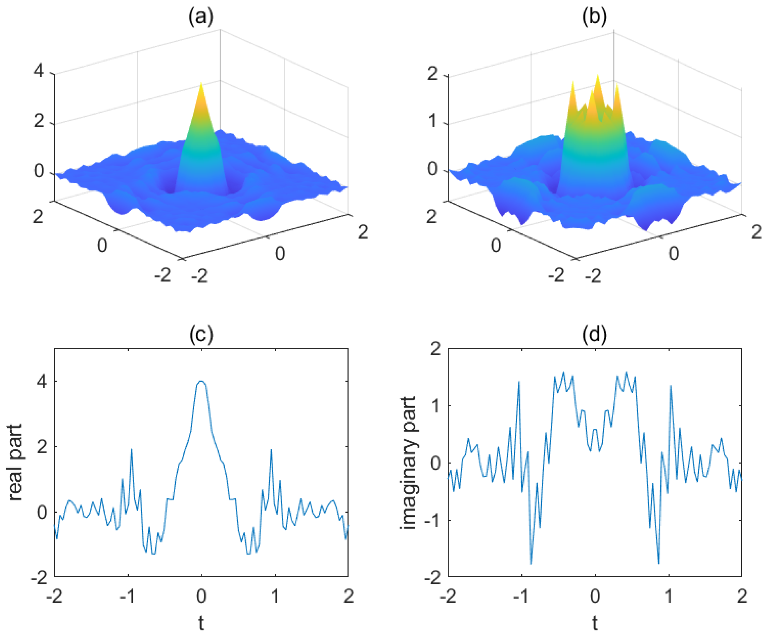
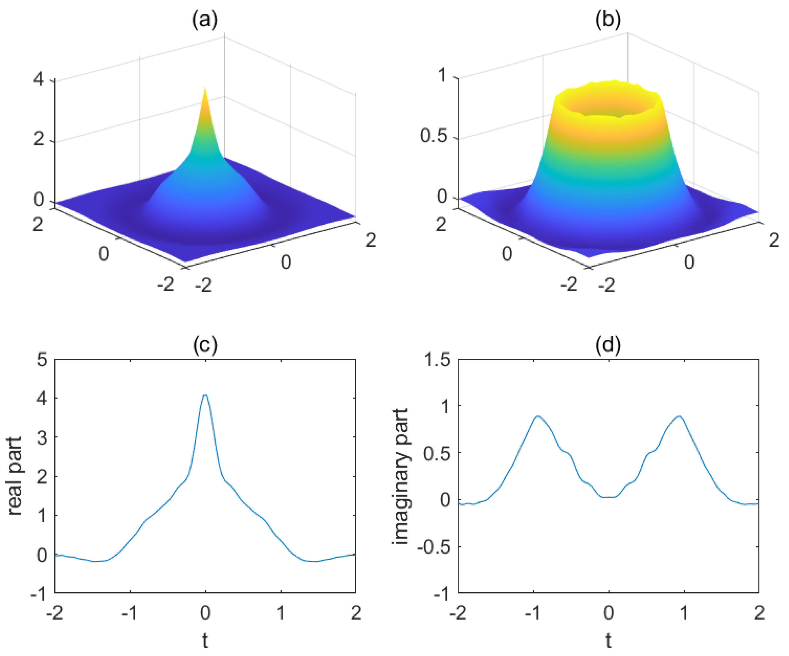
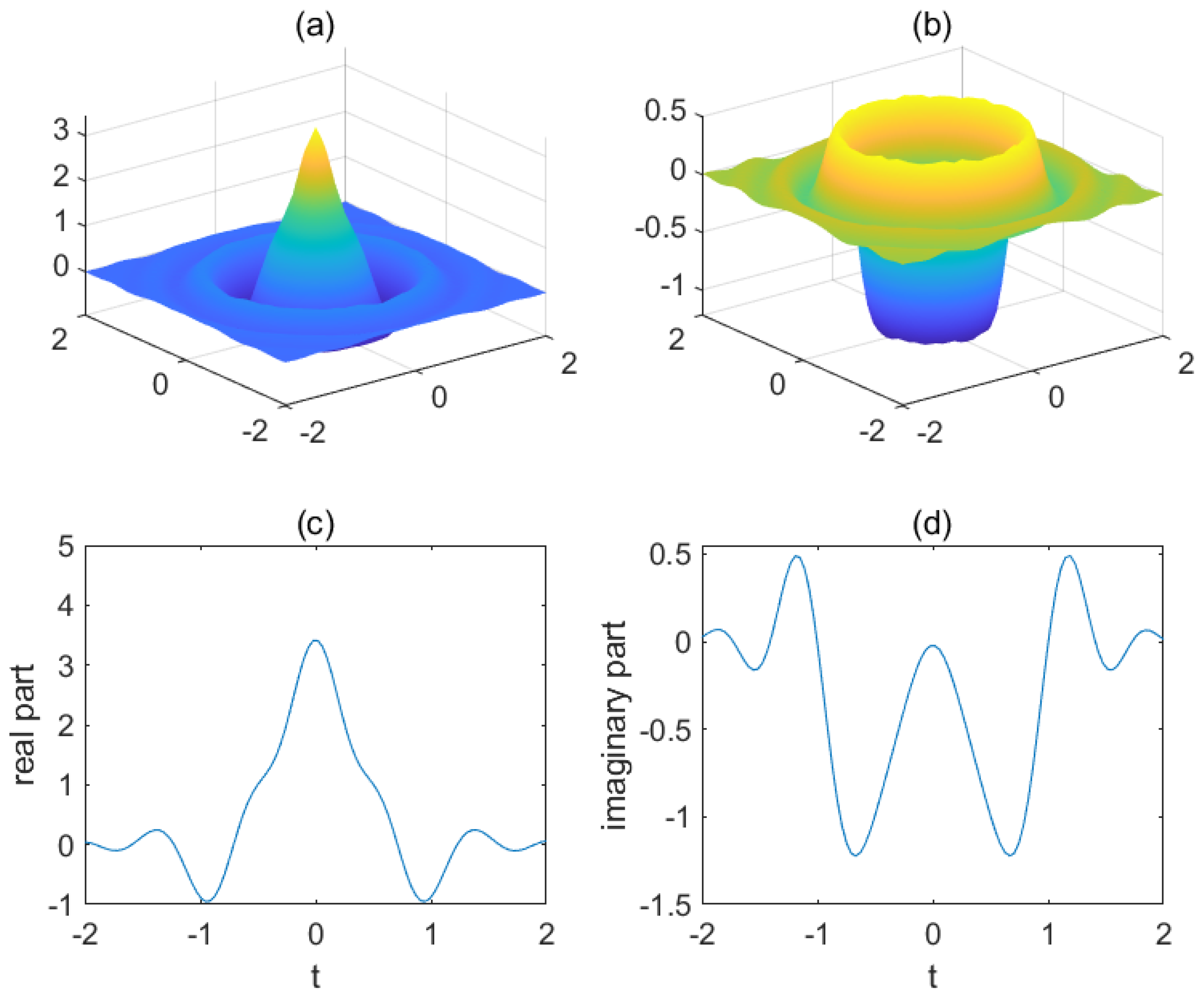
In this section, we give a specific function to illustrate the initial problem of heat equation with chirp function. In Example 2, let

$$\begin{array}{c}\hfill f\left(\mathit{x}\right)=\left\{\begin{array}{c}{e}^{-i\pi \left(x_1^2\cot {\alpha }_1+x_2^2\cot {\alpha }_2\right)}{\left(x_1^2+x_2^2\right)}^{-\frac{1}{6}},0<\left|\mathit{x}\right|<1,\hfill \\ \\ e^{-i\pi \left(x_1^2\cot {\alpha }_1+x_2^2\cot {\alpha }_2\right)}{\left(x_1^2+x_2^2\right)}^{-3},\left|\mathit{x}\right|\ge 1.\hfill \end{array}\right.\end{array}$$

It is obvious that

$$f\left(\mathit{x}\right)\in L^3\left({\mathbb{R}}^2\right),\underset{y\to 0}{lim}{v}_{\mathit{\alpha }}(\mathit{x},y)=f\left(\mathit{x}\right).$$

Let

$$g_{\mathit{\alpha }}(\mathit{x},y)=e_{\mathit{\alpha }}\left(\mathit{x}\right)v_{\mathit{\alpha }}(\mathit{x},y).$$

On the one hand, by fixing $y=0.01$, we investigate the effect of ${\alpha }_1,{\alpha }_2$. We take ${\alpha }_1={\alpha }_2=\frac{\pi }{10},\frac{\pi }{5}$ and $\frac{\pi }{2}$, respectively. Then, we can describe $g_{\mathit{\alpha }}(\mathit{x},y)$ in Figure 1, Figure 2 and Figure 3. In fact, when ${\alpha }_1={\alpha }_2=\frac{\pi }{2}$, we have $e_{(\frac{\pi }{2},\frac{\pi }{2})}\left(\mathit{x}\right)=1$, which is the case of classical heat equation. From Figure 1, Figure 2 and Figure 3, it is clear that the smaller ${\alpha }_1,{\alpha }_2$ are, the stronger the vibration of $g_{\mathit{\alpha }}(\mathit{x},y)$ is.

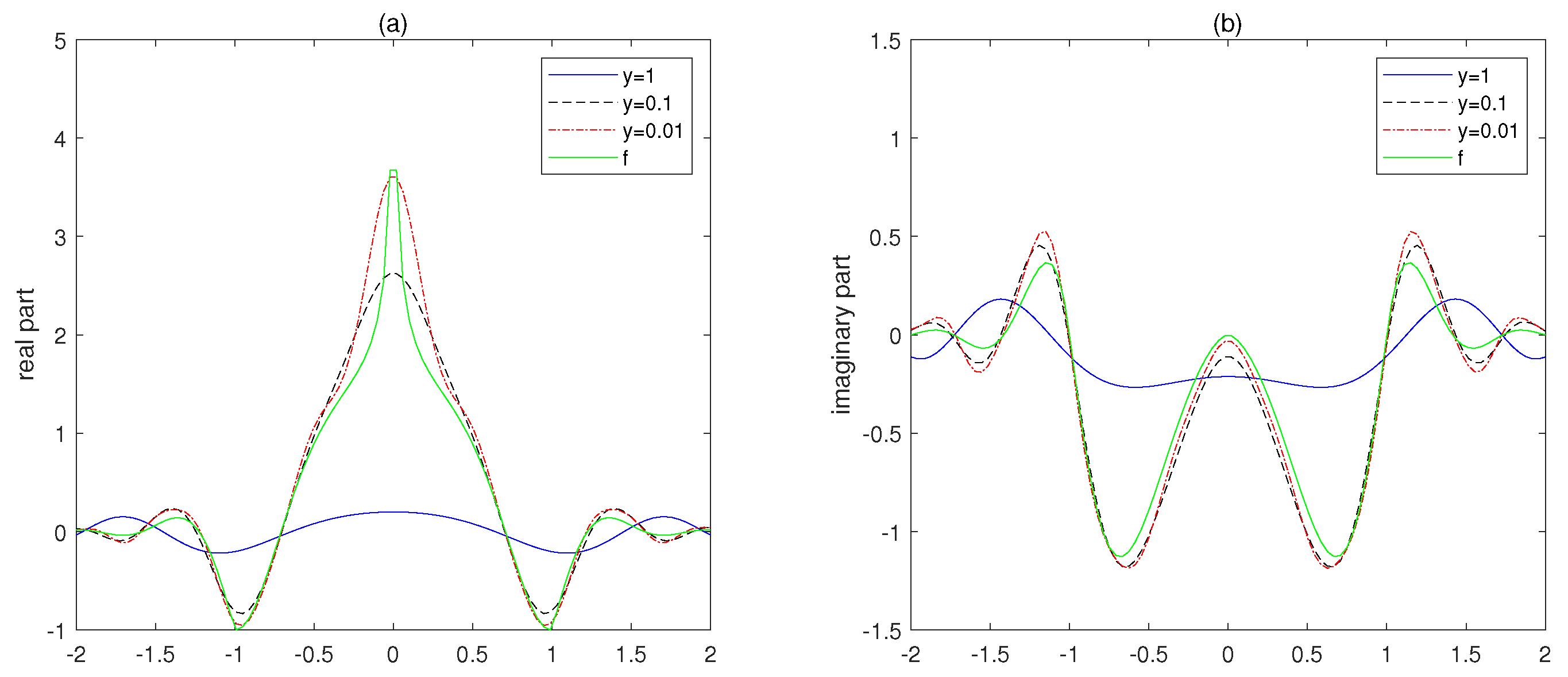
On the other hand, by fixing ${\alpha }_1={\alpha }_2=\frac{\pi }{3}$, we investigate the effect of y in the approximation. we take different $y=1,0.1$ and $0.01$. As $y\to 0$, $v_{\alpha }(\mathit{x},y)$ tends to $f\left(\mathit{x}\right)$ and this trend can be seen clearly from the sectional views in Figure 4.

5. Conclusions

This paper gives two approximation theorems in $L^p\left({\mathbb{R}}^n\right)$ via the multidimensional fractional convolution related to the FRFT. The first one is that the multidimensional fractional convolution of an $L^p$ function f and a regular $L^1$ function can approximate f in $L^p$ norm. The second one is that the multidimensional fractional convolution of an $L^p$ function f and an $L^1$ function satisfying certain conditions can approximate f point by point. As applications of the second approximation theorem, we verify solutions to the Laplace equation with the Dirichlet boundary condition and the heat equation with the initial value condition in the upper half-space. In addition, through a specific initial value function, we illustrate both the influence of the Chirp function’s index on the smoothness of the solution, and the approximation speed of the solution to the initial value.

References

- Durak, L.; Aldirmaz, S. Adaptive fractional Fourier domain filtering. Signal Process. 2010, 90, 1188–1196. [Google Scholar] [CrossRef]
- Sejdić, E.; Djurović, I.; Stanković, L. Fractional Fourier transform as a signal processing tool: An overview of recent developments. Signal Process. 2011, 91, 1351–1369. [Google Scholar] [CrossRef]
- Gómez, A.; Ugarte, J.P.; Tobón, C. The fractional Fourier transform as a biomedical signal and image processing tool: A review. Biocybern. Biomed. Eng. 2020, 40, 1081–1093. [Google Scholar] [CrossRef]
- Kumar, S.; Saxena, R.; Singh, K. Fractional Fourier transform and fractional-order calculus-based image edge detection. Circuits Syst Signal Process. 2017, 36, 1493–1513. [Google Scholar] [CrossRef]
- Saxena, N.; Sharma, K.K. Pansharpening scheme using filtering in twodimensional discrete fractional Fourier transform. IET Image Process. 2018, 12, 1013–1019. [Google Scholar] [CrossRef]
- Bernardo, L.M.; Soares, O.D.D. Fractional Fourier transforms and imaging. J. Opt. Soc. Am. A 1994, 11, 2622–2626. [Google Scholar] [CrossRef]
- Liu, S.; Ren, H.; Zhang, J.; Zhang, X. Image-scaling problem in the optical fractional Fourier transform. Appl. Opt. 1997, 36, 5671–5674. [Google Scholar] [CrossRef] [PubMed]
- Ozaktas, H.M.; Aytr, O. Fractional Fourier domains. Signal Process. 1995, 22, 119–124. [Google Scholar] [CrossRef]
- Li, J.; Sha, X.; Fang, X.; Mei, L. 8-Weighted-type fractional Fourier transform based three-branch transmission method. China Commun. 2018, 15, 147–159. [Google Scholar] [CrossRef]
- Li, Y.; Song, Z.; Sha, X. The multi-weighted type fractional Fourier transform scheme and its application over wireless communications. J. Wireless Com. Netw. 2018, 2018, 41. [Google Scholar] [CrossRef]
- Zhou, L.; Zhao, Q.; Chi, S.; Li, Y.; Liu, L.; Yu, Q. A fractional Fourier transform-based channel estimation algorithm in single-carrier direct sequence code division multiple access underwater acoustic communication system. Int. J. Distrib. Sens. Netw. 2019, 15, 11. [Google Scholar] [CrossRef]
- Namias, V. The fractional order Fourier transform and its application to quantum mechanics. IMA J. Appl. Math. 1980, 25, 241–265. [Google Scholar] [CrossRef]
- Raymer, M.G.; Beck, M.; McAlister, D. Complex wave-field reconstruction using phase-space tomography. Phys. Rev. Lett. 1994, 72, 1137–1140. [Google Scholar] [CrossRef] [PubMed]
- Wiener, N. Hermitian polynomials and Fourier analysis. J. Math. Phys. 1980, 8, 70–73. [Google Scholar] [CrossRef]
- Stein, E.M.; Weiss, G. Introduction to Fourier Analysis on Euclidean Spaces; Princeton University Press: Princeton, NJ, USA, 1971. [Google Scholar]
- Ozaktas, H.M.; Zalevsky, Z.; Kutay, M. The Fractional Fourier Transform: With Applications in Optics and Signal Processing; Wiley: New York, NY, USA, 2001. [Google Scholar]
- Kamalakkannan, R.; Roopkumar, R. Multidimensional fractional Fourier transform and generalized fractional convolution. Integral Transforms Spec. Funct. 2020, 31, 152–165. [Google Scholar] [CrossRef]
- Chen, W.; Fu, Z.W.; Grafakos, L.; Wu, Y. Fractional Fourier transforms on Lp and applications. Appl. Comput. Harmon. Anal. 2021, 55, 71–96. [Google Scholar] [CrossRef]
- Zayed, A.I. Two-dimensional fractional Fourier transform and some of its properties. Integral Transform. Spec. Funct. 2018, 29, 553–570. [Google Scholar] [CrossRef]
- Mustard, D. Fractional convolution. J. Aust. Math. Soc. B 1998, 13, 257–265. [Google Scholar] [CrossRef]
- Zayed, A.I. A convolution and product theorem for the fractional Fourier transform. IEEE Signal Process. Lett. 1998, 5, 101–103. [Google Scholar] [CrossRef]
- Zhang, Y.; Li, W. Fractional Fourier transform on R2 and an application. Front. Math. China. 2021. [Google Scholar] [CrossRef]
- Ding, Y. Foundations of Modern Analysis, 2nd ed.; Beijing Normal University Publishers: Beijing, China, 2013. [Google Scholar]