Mathematical Modeling of COVID-19 Transmission Using a Fractional Order Derivative

Abstract

In this article, the mathematical model of COVID-19 is analyzed in the sense of a fractional order Caputo operator with the consideration of an asymptomatic class. The suggested model is comprised of four compartments. The results from fixed point theory are used to theoretically analyze the existence and uniqueness of solution of the model in fractional perspective. For the numerical approximation of the suggested problem, a numerical iterative scheme is used, which is based on the Newton polynomial interpolation. For the efficiency and applicability of the suggested technique with a fractional Caputo operator, we simulate the results for various fractional orders.

1. Introduction

Wuhan, China, was the first to be infected with the new virus (2019-nCoV), which is extremely pathogenic and transmissible. This unique illness has spread over the world, causing severe acute respiratory syndrome.The COVID-19 epidemic has attracted much attention, since the first case of COVID-19 was detected. Unfortunately, the globe has reached a gloomy coronavirus milestone as of 20 December 2021, with 5.36 million fatalities recorded and confirmed cases of about 275.6 million. The total deaths have far outpaced that of the other two coronaviruses (severe acute respiratory syndrome coronavirus, SARS-CoV, and Middle East respiratory syndrome coronavirus, MERS-CoV), according to [1,2]. The worldwide epidemic is ongoing, wreaking havoc on public health and the economy throughout the world. Despite the country’s collective efforts, China’s COVID-19 pandemic has not been effectively contained. The influence of international imports and population movement (particularly among subclinical patients) on contagious control, on other hand, cannot be overlooked. It is critical to build a model for the contagion as a potent instrument to study the mechanisms of contagious disease control and transmission, in order to control contagious diseases and limit their incidence. When COVID-19 was first discovered, researchers employed epizootic data or dynamic models, as well as the effective times of COVID-19’s reproduction to predict the epidemic’s peak timing and size both locally and internationally [3,4]. Researchers also created forecast models on the impact of resuming work on the progression of the disease in Hubei Province, if not the entire country [5]. Asamoah et al. studied the global stability and cost-effectiveness of COVID-19, with the consideration of the environmental impact using Ghana’s data [6].

The early research lacked adequate raw data. As a result, the majority of these researched forecasts of the pandemic scenario differed from the actual reality.

More crucially, these investigations ignored the novel coronavirus’s high conveyance capability throughout the incubation phase, subclinical infection, and the effect of population movement on the epidemic conveyance. After extensive study on the new coronavirus pneumonia, it was oberved that social distancing had a strong impact on decreasing the number of infections. For this, several works have been presented; for instance, Qian et al. worked on COVID-19 and social distancing [7], Mwalili studied an SEIR COVID-19 model by incorporating social distancing and environment [8], Elgazzar presented the controling of COVID-19 through social distancing and awareness [9].

Most academics included the conveyance characteristics of individuals with a latent period or subclinical diseases into new coronavirus pneumonia models in later investigations [10]. Mandal et al. [11] developed a model that included a quarantine class and government action. This study found that the most important component in attaining disease management was minimizing the exposure to exposed and vulnerable individuals. Khan and Atangana et al. [12] devised a new mathematical model for COVID-19 dynamics in the presence of quarantine and isolation. Some researchers have proposed mathematical models to investigate COVID-19’s proliferation and conveyance in the community, particularly the role of asymptomatic infected persons. The authors of [13] suggested the COVID-19 spread using a constituent mathematical model in order to concentrate on super-spreaders’ contagiousness. However, only the infectiousness of exposed people was included in this model, not the infectiousness of asymptomatic people with illnesses. Indeed, research employing data from early Chinese reports paired with Bayesian inference methodology found that asymptomatic illnesses increased the epidemic’s spread [14]. Furthermore, a great number of mathematical models or studies focusing on COVID-19 and other relevant subjects have been established [15]. Yet, it is uncommon to find a model that takes into account the influence of both asymptomatic infected people’s illness features and the population’s mobility on COVID-19 conveyance.

Kang et al. [16] provided a simplified mathematical model, which could be utilized to observe the influence of the mobility of the population and subclinical infected persons on the development of COVID-19. As opposed to the other models described above, they took into account the following assumptions. To begin with, because symptomatic infected people have apparent ailments, they will be segregated and treated as soon as they are discovered. This indicates that the rate of viral infection in susceptible persons from symptomatic diseases is relatively low. As a result, the infection rate from symptomatic illnesses to vulnerable persons was overlooked. Second, since May, the pandemic situation in the provinces has mostly stabilized. This also suggests that in China, both the medical issues and the treatment methods have remained relatively steady. As a result, our model incorporated the constant cure rate. However, when people return to regular life, the chance of an epidemic re-emerging cannot be overlooked due to the large population, particularly asymptomatic persons. They then concentrated on the influence of population movement on the epidemic’s progression. Furthermore, recurrence incidences in people who have been cured are quite rare. As a result, they believed that there was no transfer of recovery to the vulnerable population.

In assessing the dynamics of an infectious disease, epidemic models of fractional order are more informative and reliable than typical integer order models, and they are being used more frequently [17,18]. For some diseases, fractional order models exhibit a substantially superior match to the real data. Many fractional operators were suggested in [19,20]; these fractional operators’ applications were presented in [21,22,23]. The Caputo operator has been used by several researchers to analyze a variety of real world phenomena. For instance, Saifullah et al. investigated a nonlinear wave model in [24], Khan et al. studied a four dimensional dynamical system with Caputo’s operator [25]. Similarly, Alqahtani et al. analyzed the bioethanol production model under a generalized nonlocal operator in the Caputo sense [26]. Furthermore, in [27], for instance, they investigated equations of fractional diffusion and their analysis. The authors of [28] employed a novel approach for numerically solving fractional order differential equations. In [29], the authors studied the nonlinear wave equation with solitary/shock solutions. In [30], the author investigated coronavirus modeling, simulations, and potential control using a mathematical model. The authors recently investigated the fractional derivative analysis of the coronavirus model [31]. The authors of [32] investigated a mathematical model to study COVID-19 and its control analysis. Several authors have conducted work on fractional differential equations [33,34,35].

We reformulated the model [16] in this paper using the Caputo derivative with a nonlinear incidence rate and fixed input and fixed treatment rates. Fractional order models provide a deeper grasp of the epidemic and provide additional insights. The remainder of the paper is organized as follows: Section 2 presents the basic preliminaries, and Section 3 presents the model formulation in terms of the parameter estimates and curve fitting. Section 4 gives the model derivation. The model’s analysis is presented in Section 5, whereas numerical simulations are shown in Section 6. Section 7 has brief concluding remarks.

2. Preliminaries

Definition 1. 

We consider $\mathsf{U}(\mathsf{t})$ to be a continuous function; then, the definition of a Caputo operator of order α, where $m-1<\alpha \le 1$ is

$$\begin{array}{c}\hfill {}_0^C{D}_{\mathsf{t}}^{\alpha }\mathsf{U}(\mathsf{t})=\frac{1}{\Gamma (m-\alpha )}{\int }_0^{\mathsf{t}}{(\mathsf{t}-\tau )}^{m-\alpha -1}\left[{\mathsf{U}}^{{}^{\prime }}(\tau )\right]\mathsf{d}\tau .\end{array}$$

Definition 2. 

We consider $\mathsf{U}(\mathsf{t})$ to be a continuous function; then, the definition of the Riemann–Liouville integration with respect to $\mathsf{t}$ is

$$\begin{array}{c}\hfill {}_0^R{\mathsf{I}}_{\mathsf{t}}^{\alpha }\mathsf{U}(\mathsf{t})=\frac{1}{\Gamma (\alpha )}{\int }_0^{\mathsf{t}}{(\mathsf{t}-\tau )}^{\alpha -1}\mathsf{U}(ø)\mathsf{d}\tau ,\alpha >0,\end{array}$$

with a converging integral.

3. Classical Integer Order Model Formulation

Here, we examine the $\mathsf{SAIR}$ mathematical model, which models COVID-19’s dynamic conveyance in mobile populations. Susceptible individuals $\mathsf{S}(\mathsf{t})$, asymptomatic people $\mathsf{A}(\mathsf{t})$, symptomatic individuals $\mathsf{I}(\mathsf{t})$, and recovered individuals $\mathsf{R}(\mathsf{t})$ make up the population size $\mathsf{N}(\mathsf{t})$. The following is a system of ordinary differential equations [16].

$$\begin{array}{c}\hfill \left\{\begin{array}{c}\frac{\mathsf{d}\mathsf{S}(\mathsf{t})}{\mathsf{d}(\mathsf{t})}=\Pi -\frac{⋏\mathsf{A}(\mathsf{t})\mathsf{S}(\mathsf{t})}{\mathsf{N}(\mathsf{t})}-\upsilon \mathsf{S}(\mathsf{t}),\hfill \\ \frac{\mathsf{d}\mathsf{A}(\mathsf{t})}{\mathsf{d}(\mathsf{t})}=\frac{⋏\mathsf{A}(\mathsf{t})\mathsf{S}(\mathsf{t})}{\mathsf{N}(\mathsf{t})}-\upsilon \mathsf{A}(\mathsf{t})-{\mathsf{q}}_{\mathsf{1}}\mathsf{A}(\mathsf{t})-{\mathsf{q}}_{\mathsf{2}}\mathsf{A}(\mathsf{t}),\hfill \\ \frac{\mathsf{d}\mathsf{I}(\mathsf{t})}{\mathsf{d}(\mathsf{t})}={\mathsf{q}}_{\mathsf{1}}\mathsf{A}(\mathsf{t})-\upsilon \mathsf{I}(\mathsf{t})-\kappa \mathsf{I}(\mathsf{t})-\nu \mathsf{I}(\mathsf{t})\hfill \\ \frac{\mathsf{d}\mathsf{R}(\mathsf{t})}{\mathsf{d}(\mathsf{t})}={\mathsf{q}}_{\mathsf{2}}\mathsf{A}(\mathsf{t})+\nu \mathsf{I}(\mathsf{t})-\upsilon \mathsf{R}(\mathsf{t}).\hfill \end{array}\right.\end{array}$$

(1)

The starting state was $\mathsf{S}(\mathsf{0})>0,\mathsf{A}(\mathsf{0})\ge 0,\mathsf{I}(\mathsf{0})\ge 0,$ and $\mathsf{R}(\mathsf{0})\ge 0$. The comprehensive input rate was represented by the parameter $\Pi >0$, and $\upsilon >0$ represented the natural death rate. The death rate owing to disease was denoted by $\kappa >0$. Vertical conveyance was not taken into account in this model; therefore, all babies were at risk. Asymptomatic infections, according to clinical practice, are not in need of therapy; yet, this population is a main infection source. The rate of asymptomatic people who have recovered becoming symptomatic was determined by the parameter ${\mathsf{q}}_{\mathsf{1}}$. ⋏ represented the transmission rate between asymptomatic and susceptible people. The rate at which asymptomatic people recover was determined by parameter ${\mathsf{q}}_2>0$. The rate at which symptomatic people recover was $\nu >0$. In clinical terms, the recurrence in treated patients is uncommon. As a result, from recovered people, no conveyance to the vulnerable class was envisaged in this model. The authors in [16] studied the local and global stability based on the disease-free as well as the endemic equilibrium points by constructing an appropriate Lyapunov function under appropriate parameter conditions. Moreover, some important results have been presented and verified by numerical simulations.

4. Model Derivation in the Caputo Operator

We used a Caputo fractional derivative to reformulate the COVID-19 model (1) to study the memory effects and learn more about the epidemic. The following is a system of Caputo fractional differential equations. Moreover, to obtain the same dimension on both sides of the coefficient, we included one auxiliary parameter $\Lambda$ [36,37,38]

$$\begin{array}{c}\hfill \left\{\begin{array}{c}{\frac{1}{{\Lambda }^{1-\alpha }}}^{\mathsf{C}}{\mathsf{D}}_{\mathsf{t}}^{\alpha }\mathsf{S}(\mathsf{t})=\Pi -\frac{⋏\mathsf{A}(\mathsf{t})\mathsf{S}(\mathsf{t})}{\mathsf{N}(\mathsf{t})}-\upsilon \mathsf{S}(\mathsf{t}),\hfill \\ {\frac{1}{{\Lambda }^{1-\alpha }}}^{\mathsf{C}}{\mathsf{D}}_{\mathsf{t}}^{\alpha }\mathsf{A}(\mathsf{t})=\frac{⋏\mathsf{A}(\mathsf{t})\mathsf{S}(\mathsf{t})}{\mathsf{N}(\mathsf{t})}-\upsilon \mathsf{A}(\mathsf{t})-{\mathsf{q}}_{\mathsf{1}}\mathsf{A}(\mathsf{t})-{\mathsf{q}}_{\mathsf{2}}\mathsf{A}(\mathsf{t}),\hfill \\ {\frac{1}{{\Lambda }^{1-\alpha }}}^{\mathsf{C}}{\mathsf{D}}_{\mathsf{t}}^{\alpha }\mathsf{I}(\mathsf{t})={\mathsf{q}}_{\mathsf{1}}\mathsf{A}(\mathsf{t})-\upsilon \mathsf{I}(\mathsf{t})-\kappa \mathsf{I}(\mathsf{t})-\nu \mathsf{I}(\mathsf{t})\hfill \\ {\frac{1}{{\Lambda }^{1-\alpha }}}^{\mathsf{C}}{\mathsf{D}}_{\mathsf{t}}^{\alpha }\mathsf{R}(\mathsf{t})={\mathsf{q}}_{\mathsf{2}}\mathsf{A}(\mathsf{t})+\nu \mathsf{I}(\mathsf{t})-\upsilon \mathsf{R}(\mathsf{t}),\hfill \end{array}\right.\end{array}$$

(2)

with $\mathsf{S}(\mathsf{0})>0,\mathsf{A}(\mathsf{0})\ge 0,\mathsf{I}(\mathsf{0})\ge 0,$ and $\mathsf{R}(\mathsf{0})\ge 0$.

5. Analysis of the Model

5.1. Existence Results

Here, the existence and uniqueness of the solution of Model (2) are presented using some fixed point results. For this purpose, Model (2) can be written as

$$\begin{array}{c}\hfill \left\{\begin{array}{c}{\frac{1}{{\Lambda }^{1-\alpha }}}^C{\mathcal{D}}_{\mathsf{t}}^{\alpha }\mathsf{S}(\mathsf{t})={\mathcal{G}}_1(\mathsf{t},\mathsf{S}),\hfill \\ {\frac{1}{{\Lambda }^{1-\alpha }}}^C{\mathcal{D}}_{\mathsf{t}}^{\alpha }\mathsf{A}(\mathsf{t})={\mathcal{G}}_2(\mathsf{t},\mathsf{A}),\hfill \\ {\frac{1}{{\Lambda }^{1-\alpha }}}^C{\mathcal{D}}_{\mathsf{t}}^{\alpha }\mathsf{I}(\mathsf{t})={\mathcal{G}}_3(\mathsf{t},\mathsf{I}),\hfill \\ {\frac{1}{{\Lambda }^{1-\alpha }}}^C{\mathcal{D}}_{\mathsf{t}}^{\alpha }\mathsf{R}(\mathsf{t})={\mathcal{G}}_4(\mathsf{t},\mathsf{R}).\hfill \end{array}\right.\end{array}$$

(3)

System (3) may be expressed as

$$\begin{array}{c}\hfill \left\{\begin{array}{c}{\frac{1}{{\Lambda }^{1-\alpha }}}^C{\mathcal{D}}_{\mathsf{t}}^{\alpha }\mathcal{F}(t)=\mathcal{H}(t,\mathcal{F}(t))\hfill \\ \mathcal{F}(0)={\mathcal{F}}_0\hfill \end{array}\right.,\end{array}$$

(4)

where

$$\begin{array}{c}\hfill \mathcal{F}(\mathsf{t})=\left\{\begin{array}{c}\mathsf{S}(\mathsf{t}),\hfill \\ \mathsf{A}(\mathsf{t}),\hfill \\ \mathsf{I}(\mathsf{t}),\hfill \\ \mathsf{R}(\mathsf{t}).\hfill \end{array}\right.\mathcal{H}(t,\mathcal{F}(t))=\left\{\begin{array}{c}{\mathcal{G}}_1,\hfill \\ {\mathcal{G}}_2,\hfill \\ {\mathcal{G}}_3,\hfill \\ {\mathcal{G}}_4.\hfill \end{array}\right.\end{array}$$

Now, to define an orbitally complete metric space, let $(\mathsf{H},\mathsf{d})$ represent the metric space and $\mathfrak{T}:\mathsf{H}\to \mathsf{H}$; if ${\mathsf{x}}_0\in \mathsf{H}$, then the orbit of ${\mathsf{x}}_0$ is the set

$$\begin{array}{ccc}\hfill O({\mathsf{x}}_0)& =& \{{\mathfrak{T}}^n{\mathsf{x}}_0:n=0,1,2,3\cdots \},\hfill \end{array}$$

where ${\mathfrak{T}}^n$ is the nth iteration of $\mathfrak{T}$, and $\mathcal{D}({\mathsf{x}}_0)$ is the diameter of $O(x_0)$. If all Cauchy sequences belonging to $O(x)$ converge in $\mathsf{H}$ for some $\mathsf{x}\in \mathsf{H}$, then $(\mathsf{H},\mathsf{d})$ is known as $\mathfrak{T}$-orbitally complete metric space.

Theorem 1 

([39]). Let $(\mathsf{H},\mathsf{d})$ represent $\mathfrak{T}$-orbitally complete metric space, $\mathfrak{T}:\mathsf{H}\to \mathsf{H}$, and $\theta :\mathsf{H}\to \mathcal{N}$; if $\exists \nu >0$ and ${\mathsf{x}}_0\in \mathsf{H}$, with $0<\mathcal{D}<\infty$, such as

$$\begin{array}{ccc}\hfill \mathsf{d}({\mathfrak{T}}^{\theta (\mathsf{x})}(\mathfrak{p}),{\mathfrak{T}}^{\theta (\mathsf{x})}(\mathfrak{q}))& \le & e^{\nu }\mathsf{d}(\mathfrak{p},\mathfrak{q}),\hfill \end{array}$$

then $\mathfrak{T}$ has a unique fixed point.

Let $\mathsf{H}=\mathrm{C}\times \mathrm{C}\times \mathrm{C}$, where $\mathrm{C}\left([0,\mathrm{T}],\mathcal{R}\right)$ represents space containing continuous mappings, and $\mathsf{d}(\mathfrak{p},\mathfrak{q})={sup}_{\mathsf{t}\in [0,\mathrm{T}]}|\mathfrak{p}-\mathfrak{q}|$ is the metric on $\mathsf{H}$.

The existence and uniqueness of the solution of the problem (4) are presented and proved in the following theorem.

Theorem 2. 

Let $\mathfrak{T}:\mathsf{H}\to \mathsf{H}$ be defined by $\mathfrak{T}(\mathcal{F}(t))={\mathcal{F}}_0+\frac{1-\alpha }{\Gamma (\alpha )}{\int }_0^{\mathsf{t}}{(\mathsf{t}-\tau )}^{\alpha -1}\mathsf{H}(\tau ,\mathfrak{F}(\tau ))\mathsf{d}\tau$ and

$$|\mathsf{H}(\mathsf{t},\mathcal{F}(t))-\mathsf{H}(\mathsf{t},\mathcal{K}(t))|\le \frac{\Gamma (\alpha +1)}{\alpha {\widehat{\mathsf{T}}}^{\alpha }}{e}^{-\nu }|\sqrt{|\mathcal{F}|}-\sqrt{|\mathcal{K}|}|$$

$$|\mathsf{H}(\mathsf{t},\mathcal{F}(t))-\mathsf{H}(\mathsf{t},\mathcal{K}(t))|\le \frac{\Gamma (\alpha +1)}{\alpha {\widehat{\mathsf{T}}}^{\alpha }}{e}^{-\nu }|\sqrt{|\mathcal{F}|}+\sqrt{|\mathcal{K}|}|.$$

Then, there must be a unique solution to problem (4).

Proof. 

By applying the integral on Equation (4), we obtain

$$\begin{array}{ccc}\hfill \mathcal{F}(\mathsf{t})& =& {\mathcal{F}}_0+\frac{1-\alpha }{\Gamma (\alpha )}{\int }_0^{\mathsf{t}}{(\mathsf{t}-\tau )}^{\alpha -1}\mathsf{H}(\tau ,\mathcal{F}(t))\mathsf{d}\tau =\mathfrak{T}\mathcal{F}.\hfill \end{array}$$

(5)

To prove that there exists a unique fixed point of $\mathfrak{T},$

$$\begin{array}{ccc}\hfill |\mathfrak{T}\mathcal{F}-\mathfrak{T}\mathcal{K}|& =& \left|\frac{1-\alpha }{\Gamma (\alpha )}{\int }_0^{\mathsf{t}}{(\mathsf{t}-\tau )}^{\alpha -1}(\mathsf{H}(\tau ,\mathcal{F}))\mathsf{d}\tau \right|\hfill \\ & \le & \frac{1-\alpha }{\Gamma (\alpha )}{\int }_0^{\mathsf{t}}{(\mathsf{t}-\tau )}^{\alpha -1}|\mathsf{H}(\tau ,\mathcal{F})-\mathsf{H}(\tau ,\mathcal{K}))|\mathsf{d}\tau \hfill \\ & \le & \frac{\Gamma (\alpha +1)e^{-\nu }}{\Gamma (\alpha ){\widehat{\mathsf{T}}}^{\alpha }}{\int }_0^{\mathsf{t}}{(\mathsf{t}-\tau )}^{\alpha -1}|\sqrt{|\mathcal{F}|}-\sqrt{|\mathcal{K}|}|\mathsf{d}\tau \hfill \\ & =& \frac{\alpha e^{-\nu }}{{\widehat{\mathsf{T}}}^{\alpha }}\underset{\mathsf{t}\in [0,\mathrm{T}]}{sup}|\sqrt{|\mathcal{F}|}-\sqrt{|\mathcal{K}|}|{\int }_0^{\mathsf{t}}{(t-\tau )}^{\alpha -1}\mathsf{d}\tau \hfill \\ & \le & e^{-\nu }\underset{\mathsf{t}\in [0,\mathrm{T}]}{sup}|\sqrt{|\mathcal{F}|}-\sqrt{|\mathcal{K}|}|.\hfill \end{array}$$

Moreover,

$$\begin{array}{ccc}\hfill |\mathfrak{T}\mathcal{F}|+|\mathfrak{T}\mathcal{K}|& =& \left|\frac{1-\alpha }{\Gamma (\alpha )}{\int }_0^{\mathsf{t}}{(\mathsf{t}-\tau )}^{\alpha -1}(\mathsf{H}(\tau ,\mathcal{F}))\mathsf{d}\tau |+|\frac{1}{\Gamma (\alpha )}{\int }_0^{\mathsf{t}}{(\mathsf{t}-\tau )}^{\alpha -1}(\mathsf{H}(\tau ,\mathcal{K}))\mathsf{d}\tau \right|\hfill \\ & \le & \frac{1-\alpha }{\Gamma (\alpha )}{\int }_0^{\mathsf{t}}{(\mathsf{t}-\tau )}^{\alpha -1}(|\mathsf{H}(\tau ,\mathcal{F})|+|\mathsf{H}(\tau ,\mathcal{K})|)\mathsf{d}\tau \hfill \\ & \le & \frac{\Gamma (\alpha +1)e^{-\nu }}{\Gamma (\alpha ){\widehat{\mathsf{T}}}^{\alpha }}{\int }_0^{\mathsf{t}}{(\mathsf{t}-\tau )}^{\alpha -1}|\sqrt{|\mathcal{F}|}+\sqrt{|\mathcal{K}|}|\mathsf{d}\tau \hfill \\ & =& \frac{\alpha e^{-\nu }}{{\widehat{\mathsf{T}}}^{\alpha }}\underset{\mathsf{t}\in [0,\mathrm{T}]}{sup}|\sqrt{|\mathcal{F}|}+\sqrt{|\mathcal{K}|}|{\int }_0^{\mathsf{t}}{(t-\tau )}^{\alpha -1}\mathsf{d}\tau \hfill \\ & \le & e^{-\nu }\underset{\mathsf{t}\in [0,\mathrm{T}]}{sup}|\sqrt{|\mathcal{F}|}+\sqrt{|\mathcal{K}|}|\le \underset{\mathsf{t}\in [0,\mathrm{T}]}{sup}|\sqrt{|\mathcal{F}|}+\sqrt{|\mathcal{K}|}|.\hfill \end{array}$$

Now,

$$\begin{array}{ccc}\hfill \mathsf{d}({\mathfrak{T}}^2\mathcal{F},{\mathfrak{T}}^2\mathcal{K})& =& \underset{\mathsf{t}\in [0,\mathrm{T}]}{sup}|{\mathfrak{T}}^2\mathcal{F}-{\mathfrak{T}}^2\mathcal{K}|\hfill \\ & =& \underset{\mathsf{t}\in [0,\mathrm{T}]}{sup}|\mathfrak{T}\mathcal{F}-\mathfrak{T}\mathcal{K}|\times \underset{\mathsf{t}\in [0,\mathrm{T}]}{sup}|\mathfrak{T}\mathcal{F}+\mathfrak{T}\mathcal{K}|\hfill \\ & \le & \underset{\mathsf{t}\in [0,\mathrm{T}]}{sup}|\mathfrak{T}\mathcal{F}-\mathfrak{T}\mathcal{K}|\times \underset{\mathsf{t}\in [0,\mathrm{T}]}{sup}(|\mathfrak{T}\mathcal{F}|+|\mathfrak{T}\mathcal{K}|)\hfill \\ & \le & e^{-\nu }\underset{\mathsf{t}\in [0,\mathrm{T}]}{sup}|\sqrt{|\mathcal{F}|}-\sqrt{|\mathcal{K}|}|\times sup\underset{\mathsf{t}\in [0,\mathrm{T}]}{sup}|\sqrt{|\mathcal{F}|}+\sqrt{|\mathcal{K}|}|\hfill \\ & =& e^{-\nu }\underset{\mathsf{t}\in [0,\mathrm{T}]}{sup}||\mathcal{F}|-|\mathcal{K}||\hfill \\ & \le & e^{-\nu }\underset{\mathsf{t}\in [0,\mathrm{T}]}{sup}|\mathcal{F}-\mathcal{K}|\hfill \\ & =& e^{-\nu }\mathsf{d}(\mathcal{F},\mathcal{K}).\hfill \end{array}$$

If we take $\theta :\mathsf{H}\to \mathcal{N}$, such that $\theta (\mathcal{F})=2$ for each $\mathcal{F}\in \mathsf{H}$, then all conditions of Theorem 1 hold; therefore, there exists a fixed point of $\mathfrak{T}$, which is unique, and consequently, problem (4) has a unique solution. □

5.2. Ulam–Hyers Stability

Here, we present the U-H and the generalized U-H stability [40,41] of the suggested system. Let us assume $\epsilon$, with the following inequality

$$\begin{array}{c}\hfill {|}^{\mathcal{C}}{\mathcal{D}}^p\widetilde{Ʊ}(t)-\mathcal{X}(t,\widetilde{Ʊ}(t))|\le \epsilon ,t\in \mathcal{J},\epsilon =max{({\epsilon }_i)}^T,i=1,2,3,4.\end{array}$$

(6)

Definition 3. 

System (2) is UH stable, if there exist ${\mathbf{U}}_{\mathcal{X}}>0$ for all $\epsilon >0$; then the solution of $\widetilde{Ʊ}\in \mathbf{Y}$ holds for (6); there is a unique solution $Ʊ\in \mathbf{Y}$ for Equation (4), such that

$$|\widetilde{Ʊ}(t)-Ʊ(t)|\le {\mathbf{U}}_{\mathcal{X}}\epsilon ,t\in \mathcal{J},\mathbf{U}\mathcal{X}=max{(\mathbf{U}{\mathcal{X}}_j)}^T.$$

Definition 4. 

System (2) is generalized UH stable, if there exists a continuous function $\Phi :R^{+}\to R^{+}$ and $\Phi (0)=0$, so that for all solutions $\widetilde{Ʊ}\in \mathbf{Y}$ of (6), there is a unique solution $Ʊ\in \mathbf{Y}$ for (4), with the following

$$|\widetilde{Ʊ}(t)-Ʊ(t)|\le {\Phi }_{\mathcal{X}}\epsilon ,t\in \mathcal{J},{\Phi }_{\mathcal{X}}=max{({\Phi }_{{\mathcal{X}}_j})}^T.$$

Remark 1. 

A function $\widetilde{Ʊ}\in \mathbf{Y}$ satisfies (6), if and only if there exists a function $\Phi \in \mathbf{Y}$ with the following properties:

(I) 

$|\Phi (t)|\le \epsilon ,\Phi =max({\Phi }_j),t\in \mathcal{J}$.

(II) 

${}^{\mathcal{C}}{\mathcal{D}}^p\widetilde{Ʊ}(t)=\mathcal{X}(t,\widetilde{Ʊ}(t))+\Phi (t),t\in \mathcal{J}.$

Lemma 1. 

If $\widetilde{Ʊ}\in \mathbf{Y}$ holds for Equation (6), then $\widetilde{Ʊ}$ also holds for the following

$$\begin{array}{c}\hfill |\widetilde{Ʊ}(t)-{\widetilde{Ʊ}}_0(t)-\frac{1-\alpha }{\Gamma (\alpha )}{\int }_0^t{(t-\vartheta )}^{\alpha -1}\mathcal{X}(\vartheta ,\widetilde{Ʊ}(\vartheta ))d\vartheta |\le \epsilon .\end{array}$$

(7)

Proof. 

Using (II), we have

$${}^{\mathcal{C}}{\mathcal{D}}^p\widetilde{Ʊ}(t)=\mathcal{X}(t,\widetilde{Ʊ}(t))+\Phi (t),$$

and along with Lemma 1, we obtain

$$\begin{array}{c}\hfill \widetilde{Ʊ}(t)={\widetilde{Ʊ}}_0(t)+\frac{1-\alpha }{\Gamma (\alpha )}{\int }_0^t{(t-\vartheta )}^{\alpha -1}\mathcal{X}(\vartheta ,\widetilde{Ʊ}(\vartheta ))d\vartheta +\frac{1-\alpha }{\Gamma (\alpha )}{\int }_0^t{(t-\vartheta )}^{\alpha -1}\Phi (\vartheta )d\vartheta .\end{array}$$

(8)

Next, using (I) gives

$$\begin{array}{c}\hfill \begin{array}{cc}\hfill |\widetilde{Ʊ}(t)-{\widetilde{Ʊ}}_0(t)-\frac{1-\alpha }{\Gamma (\alpha )}{\int }_0^t{(t-\vartheta )}^{\alpha -1}\mathcal{X}(\vartheta ,\widetilde{Ʊ}(\vartheta ))d\vartheta |& \le \frac{1-\alpha }{\Gamma (\alpha )}{\int }_0^t{(t-\vartheta )}^{\alpha -1}|\Phi (\vartheta )|d\vartheta \le \epsilon .\hfill \end{array}\end{array}$$

(9)

Therefore, the proof is finished. □

Theorem 3. 

For all $Ʊ\in \mathbf{Y}$, $\mathcal{X}:\mathcal{J}\times R^4\to R$ with the assumption $(C_1)$ holds, and $1-p\mathcal{L}\mathcal{X}>0$. Equation (4) is equal to Equation (2) and is UH stable and, consequently, generalized UH stable.

Proof. 

Suppose that $Ʊ,\widetilde{Ʊ}\in \mathbf{Y}$ is a unique solution of (4); therefore, for all $\epsilon >0,t\in \mathcal{J}$, along with Lemma 1, we have

$$\begin{array}{ccc}\hfill |\widetilde{Ʊ}(t)-Ʊ(t)|& =& \underset{t\in \mathcal{J}}{max}|\widetilde{Ʊ}(t)-{Ʊ}_0-\frac{1-\alpha }{\Gamma (\alpha )}{\int }_0^t{(t-\vartheta )}^{\alpha -1}\mathcal{X}(\vartheta ,Ʊ(\vartheta ))d\vartheta |\hfill \\ & \le & \underset{t\in \mathcal{J}}{max}|\widetilde{Ʊ}(t)-{\widetilde{Ʊ}}_0-\frac{1-\alpha }{\Gamma (\alpha )}{\int }_0^t{(t-\vartheta )}^{\alpha -1}\mathcal{X}(\vartheta ,Ʊ(\vartheta ))d\vartheta |\hfill \\ & +& \underset{t\in \mathcal{J}}{max}\frac{1-\alpha }{\Gamma (\alpha )}{\int }_0^t{(t-\vartheta )}^{\alpha -1}|\mathcal{X}(\vartheta ,\widetilde{Ʊ}(\vartheta ))-\mathcal{X}(\vartheta ,Ʊ(\vartheta ))|d\vartheta \hfill \\ & \le & |Ʊ(t)-{\widetilde{Ʊ}}_0-\frac{1-\alpha }{\Gamma (\alpha )}{\int }_0^t{(t-\vartheta )}^{\alpha -1}\mathcal{X}(\vartheta ,\widetilde{Ʊ}(\vartheta ))d\vartheta |+\frac{{\mathcal{L}}_{\mathcal{X}}}{\Gamma (\alpha )}{\int }_0^t{(t-\vartheta )}^{\alpha -1}|\widetilde{Ʊ}(\vartheta )-Ʊ(\vartheta )|d\vartheta \hfill \\ & \le & \alpha \epsilon +\alpha {\mathcal{L}}_{\mathcal{X}}|\widetilde{Ʊ}(t)-Ʊ(t)|,\hfill \end{array}$$

which gives

$$\begin{array}{c}\hfill \parallel \widetilde{Ʊ}-Ʊ\parallel \le {\mathbf{U}}_{\mathcal{X}}\epsilon .\end{array}$$

(10)

From (10), we may write

$$\mathbf{U}\mathcal{X}=\frac{\alpha }{1-\alpha \mathcal{L}\mathcal{X}}.$$

(11)

Hence, equating ${\Phi }_{\mathcal{X}}(\epsilon )=\mathbf{U}\mathcal{X}\epsilon$, so that $\Phi \mathcal{X}(0)=0$, we conclude that the solution of (2) is stable for both the UH and the generalized UH. □

5.3. Numerical Algorithm

Next, we establish a numerical scheme for the proposed model (2). We consider the first equation of System (3)

$$\begin{array}{ccc}\hfill {\frac{1}{{\Lambda }^{1-\alpha }}}^C{\mathcal{D}}_{\mathsf{t}}^{\alpha }\mathsf{S}(\mathsf{t})& =& {\mathcal{G}}_1(\mathsf{t},\mathsf{S}).\hfill \end{array}$$

(12)

Equation (12) can also be rearranged in the following way:

$$\begin{array}{ccc}\hfill \mathsf{S}(\mathsf{t})-\mathsf{S}(0)& =& \frac{1-\alpha }{\Gamma (\alpha )}{\int }_0^{\mathsf{t}}{\mathcal{G}}_1(\tau ,\mathsf{S}(\tau )){(\mathsf{t}-\tau )}^{\alpha -1}\mathsf{d}\tau .\hfill \end{array}$$

(13)

We can write the following at point ${\mathsf{t}}_{ı+1}=(ı+1)\Delta \mathsf{t}$:

$$\begin{array}{ccc}\hfill \mathsf{S}({\mathsf{t}}_{ı+1})-\mathsf{S}(0)& =& \frac{1-\alpha }{\Gamma (\alpha )}{\int }_0^{{\mathsf{t}}_{ı+1}}{\mathcal{G}}_1(\tau ,\mathsf{S}(\tau )){({\mathsf{t}}_{ı+1}-\tau )}^{\alpha -1}\mathsf{d}\tau .\hfill \end{array}$$

(14)

As a result,

$$\begin{array}{ccc}\hfill \mathsf{S}({\mathsf{t}}_{ı+1})& =& \mathsf{S}(0)+\frac{1-\alpha }{\Gamma (\alpha )}\sum _{\ell =2}^{ı}{\int }_{{\mathsf{t}}_{\ell }}^{{\mathsf{t}}_{\ell +1}}{\mathcal{G}}_1(\tau ,\mathsf{S}(\tau )){({\mathsf{t}}_{ı+1}-\tau )}^{\alpha -1}\mathsf{d}\tau .\hfill \end{array}$$

(15)

By substituting Equation (15) for the Newton polynomial, we obtain

$$\begin{array}{ccc}\hfill {\mathsf{S}}^{ı+1}& =& {\mathsf{S}}_0+\frac{1-\alpha }{\Gamma (\alpha )}\sum _{\ell =2}^{ı}{\int }_{{\mathsf{t}}_{\ell }}^{{\mathsf{t}}_{\ell +1}}\left\{\begin{array}{cc}& {\mathcal{G}}_1({\mathsf{t}}_{\ell -2},{\mathsf{S}}^{\ell -2})\hfill \\ & +\frac{{\mathcal{G}}_1({\mathsf{t}}_{\ell -1},{\mathsf{S}}^{\ell -1})-{\mathcal{G}}_1({\mathsf{t}}_{\ell -2},{\mathsf{S}}^{\ell -2})}{\Delta \mathsf{t}}(\tau -{\mathsf{t}}_{\ell -2})\hfill \\ & +\frac{{\mathcal{G}}_1({\mathsf{t}}_{\ell },{\mathsf{S}}^{\ell })-2{\mathcal{G}}_1({\mathsf{t}}_{\ell -1},{\mathsf{S}}^{\ell -1})({\mathcal{G}}_1({\mathsf{t}}_{\ell -2},{\mathsf{S}}^{\ell -2}))}{2{(\Delta \mathsf{t})}^2}\hfill \\ & \times (\tau -{\mathsf{t}}_{\ell -2})(\tau -{\mathsf{t}}_{\ell -1})\hfill \end{array}\right\}\hfill \\ \hfill & & \times {({\mathsf{t}}_{ı+1}-\tau )}^{\alpha -1}\mathsf{d}\tau .\hfill \end{array}$$

(16)

As a result, the preceding equation may be rearranged in the following manner:

$$\begin{array}{c}\hfill {\mathsf{S}}^{ı+1}={\mathsf{S}}_0+\frac{1-\alpha }{\Gamma (\alpha )}\sum _{\ell =2}^{ı}\left\{\begin{array}{c}{\int }_{{\mathsf{t}}_{\ell }}^{{\mathsf{t}}_{\ell +1}}{\mathcal{G}}_1({\mathsf{t}}_{\ell -2},{\mathsf{S}}^{\ell -2}){({\mathsf{t}}_{ı+1}-\tau )}^{\alpha -1}\mathsf{d}\tau \\ +{\int }_{{\mathsf{t}}_{\ell }}^{{\mathsf{t}}_{\ell +1}}\frac{{\mathcal{G}}_1({\mathsf{t}}_{\ell -1},{\mathsf{S}}^{\ell -1})-{\mathcal{G}}_1({\mathsf{t}}_{\ell -2,{\mathsf{S}}^{\ell -2}})}{\Delta \mathsf{t}}\\ (\tau -{\mathsf{t}}_{\ell -2}){({\mathsf{t}}_{ı+1}-\tau )}^{\alpha -1}\mathsf{d}\tau \\ +{\int }_{{\mathsf{t}}_{\ell }}^{{\mathsf{t}}_{\ell +1}}\frac{{\mathcal{G}}_1({\mathsf{t}}_{\ell },{\mathsf{S}}^{\ell })-2{\mathcal{G}}_1({\mathsf{t}}_{\ell -1},{\mathsf{S}}^{\ell -1})({\mathcal{G}}_1({\mathsf{t}}_{\ell -2},{\mathsf{S}}^{\ell -2}))}{2{(\Delta \mathsf{t})}^2}\\ (\tau -{\mathsf{t}}_{\ell -2})(\tau -{\mathsf{t}}_{\ell -1}){({\mathsf{t}}_{ı+1}-\tau )}^{\alpha -1}\mathsf{d}\tau \end{array}\right\}.\end{array}$$

(17)

Consequently,

$$\begin{array}{ccc}\hfill {\mathsf{S}}^{ı+1}& =& {\mathsf{S}}_0+\frac{1-\alpha }{\Gamma (\alpha )}\sum _{\ell =2}^{ı}{\mathcal{G}}_1({\mathsf{t}}_{\ell -2},{\mathsf{S}}^{\ell -2}){\int }_{{\mathsf{t}}_{\ell }}^{{\mathsf{t}}_{\ell +1}}{({\mathsf{t}}_{ı+1}-\tau )}^{\alpha -1}\mathsf{d}\tau \hfill \\ \hfill & & +\frac{1}{\Gamma (\alpha )}\sum _{\ell =2}^{ı}\frac{{\mathcal{G}}_1({\mathsf{t}}_{\ell -1},{\mathsf{S}}^{\ell -1})-{\mathcal{G}}_1({\mathsf{t}}_{\ell -2},{\mathsf{S}}^{\ell -2})}{\Delta \mathsf{t}}\hfill \\ & & \times {\int }_{{\mathsf{t}}_{\ell }}^{{\mathsf{t}}_{\ell +1}}(\tau -{\mathsf{t}}_{\ell -2}){({\mathsf{t}}_{ı+1}-\tau )}^{\alpha -1}\mathsf{d}\tau \hfill \\ \hfill & & +\frac{1}{\Gamma (\alpha )}\sum _{\ell =2}^{ı}\frac{{\mathcal{G}}_1({\mathsf{t}}_{\ell },{\mathsf{S}}^{\ell })-2{\mathcal{G}}_1({\mathsf{t}}_{\ell -1},{\mathsf{S}}^{\ell -1})+({\mathcal{G}}_1({\mathsf{t}}_{\ell -2},{\mathsf{S}}^{\ell -2}))}{2{(\Delta \mathsf{t})}^2}\hfill \\ \hfill & & \times {\int }_{{\mathsf{t}}_{\ell }}^{{\mathsf{t}}_{\ell +1}}(\tau -{\mathsf{t}}_{\ell -2})(\tau -{\mathsf{t}}_{\ell -1}){({\mathsf{t}}_{ı+1}-\tau )}^{\alpha -1}\mathsf{d}\tau .\hfill \end{array}$$

(18)

In Equation (18), we may compute the aforementioned integrals as follows:

$$\begin{array}{ccc}\hfill {\int }_{{\mathsf{t}}_{\ell }}^{{\mathsf{t}}_{\ell +1}}{({\mathsf{t}}_{ı+1}-\tau )}^{\alpha -1}\mathsf{d}\tau & =& \frac{{(\Delta \mathsf{t})}^{\alpha }}{\alpha }\left[{(ı-\ell +1)}^{\alpha }-{(ı-\ell )}^{\alpha }\right],\hfill \\ \hfill {\int }_{{\mathsf{t}}_{\ell }}^{{\mathsf{t}}_{\ell +1}}(\tau -{\mathsf{t}}_{\ell -2}){({\mathsf{t}}_{ı+1}-\tau )}^{\alpha -1}\mathsf{d}\tau & =& \frac{{(\Delta \mathsf{t})}^{\alpha +1}}{\alpha (\alpha +1)}\hfill \\ \hfill & \times & \left[\begin{array}{cc}\hfill (ı& {-\ell +1)}^{\alpha }(ı-\ell +3+2\alpha )\hfill \\ & -{(ı-\ell )}^{\alpha }(ı-\ell +3+3\alpha )\hfill \end{array}\right],\hfill \end{array}$$

(19)

$$\begin{array}{ccc}\hfill {\int }_{{\mathsf{t}}_{\ell }}^{{\mathsf{t}}_{\ell +1}}(\tau -{\mathsf{t}}_{\ell -2})(\tau -{\mathsf{t}}_{\ell -1}){({\mathsf{t}}_{ı+1}-\tau )}^{\alpha -1}\mathsf{d}\tau & =& \frac{{(\Delta \mathsf{t})}^{\alpha +2}}{\alpha (\alpha +1)(\alpha +2)}\hfill \\ \hfill & \times & \left[\begin{array}{cc}& {(ı-\ell +1)}^{\alpha }\left[\begin{array}{cc}& 2{(ı-\ell )}^2+(3\alpha +10)(ı-\ell )\hfill \\ & +2{\alpha }^2+9\alpha +12\hfill \end{array}\right]\hfill \\ & -{(ı-\ell )}^{\alpha }\left[\begin{array}{cc}& 2{(ı-\ell )}^2+(5\alpha +10)(ı-\ell )\hfill \\ & +6{\alpha }^2+18\alpha +12\hfill \end{array}\right]\hfill \end{array}\right].\hfill \end{array}$$

We may see the following strategy, if we insert these values into Equation (18):

$$\begin{array}{ccc}\hfill {\mathsf{S}}^{ı+1}& =& {\mathsf{S}}_0+\frac{{(\Delta \mathsf{t})}^{\alpha }}{\Gamma (\alpha +1)}\sum _{\ell =2}^{ı}{\mathcal{G}}_1({\mathsf{t}}_{\ell -2},{\mathsf{S}}^{\ell -2})\hfill \\ \hfill & \times & \left[{(ı-\ell +1)}^{\alpha }-{(ı-\ell )}^{\alpha }\right]\hfill \\ \hfill & +& \frac{{(\Delta \mathsf{t})}^{\alpha }}{\Gamma (\alpha +2)}\sum _{\ell =2}^{ı}\left[{\mathcal{G}}_1({\mathsf{t}}_{\ell -1},{\mathsf{S}}^{\ell -1})-{\mathcal{G}}_1({\mathsf{t}}_{\ell -2},{\mathsf{S}}^{\ell -2})\right]\hfill \\ & \times & \left[\begin{array}{cc}& {(ı-\ell +1)}^{\alpha }(ı-\ell +3+2\alpha )\hfill \\ & -{(ı-\ell )}^{\alpha }(ı-\ell +3+3\alpha )\hfill \end{array}\right]\hfill \\ \hfill & \times & +\frac{{(\Delta \mathsf{t})}^{\alpha }}{2\Gamma (\alpha +3)}\sum _{\ell =2}^{ı}\left[\begin{array}{cc}\hfill {\mathcal{G}}_1({\mathsf{t}}_{\ell },{\mathsf{S}}^{\ell }& )-2{\mathcal{G}}_1({\mathsf{t}}_{\ell -1},{\mathsf{S}}^{\ell -1})\hfill \\ & +({\mathcal{G}}_1({\mathsf{t}}_{\ell -2},{\mathsf{S}}^{\ell -2}))\hfill \end{array}\right]\hfill \\ \hfill & \times & \left[\begin{array}{cc}& {(ı-\ell +1)}^{\alpha }\left[\begin{array}{cc}& 2{(ı-\ell )}^2+(3\alpha +10)(ı-\ell )\hfill \\ & +2{\alpha }^2+9\alpha +12\hfill \end{array}\right]\hfill \\ & -{(ı-\ell )}^{\alpha }\left[\begin{array}{cc}& 2{(ı-\ell )}^2+(5\alpha +10)(ı-\ell )\hfill \\ & +6{\alpha }^2+18\alpha +12\hfill \end{array}\right]\hfill \end{array}\right].\hfill \end{array}$$

(20)

Similarly from the second, third, and fourth equations of system (12), we can write

$$\begin{array}{ccc}\hfill {\mathsf{A}}^{ı+1}& =& {\mathsf{A}}_0+\frac{{(\Delta \mathsf{t})}^{\alpha }}{\Gamma (\alpha +1)}\sum _{\ell =2}^{ı}{\mathcal{G}}_2\left({\mathsf{t}}_{\ell -2},{\mathsf{A}}^{\ell -2}\right)\left[{(ı-\ell +1)}^{\alpha }-{(ı-\ell )}^{\alpha }\right]\hfill \\ \hfill & +& \frac{{(\Delta \mathsf{t})}^{\alpha }}{\Gamma (\alpha +2)}\sum _{\ell =2}^{ı}\left[{\mathcal{G}}_2\left({\mathsf{t}}_{\ell -1},{\mathsf{A}}^{\ell -1}\right)-{\mathcal{G}}_2\left({\mathsf{t}}_{\ell -2},{\mathsf{A}}^{\ell -2}\right)\right]\hfill \\ & \times & \left[\begin{array}{cc}& {(ı-\ell +1)}^{\alpha }(ı-\ell +3+2\alpha )\hfill \\ & -{(ı-\ell )}^{\alpha }(ı-\ell +3+3\alpha )\hfill \end{array}\right]\hfill \\ \hfill & +& \frac{{(\Delta \mathsf{t})}^{\alpha }}{2\Gamma (\alpha +3)}\sum _{\ell =2}^{ı}\left[\begin{array}{cc}& {\mathcal{G}}_2\left({\mathsf{t}}_{\ell },{\mathsf{A}}^{\ell }\right)-2{\mathcal{G}}_2\left({\mathsf{t}}_{\ell -1},{\mathsf{A}}^{\ell -1}\right)\hfill \\ & +{\mathcal{G}}_2\left({\mathsf{t}}_{\ell -2},{\mathsf{A}}^{\ell -2}\right)\hfill \end{array}\right]\hfill \\ \hfill & \times & \left[\begin{array}{cc}& {(ı-\ell +1)}^{\alpha }\left[\begin{array}{cc}& 2{(ı-\ell )}^2+(3\alpha +10)(ı-\ell )\hfill \\ & +2{\alpha }^2+9\alpha +12\hfill \end{array}\right]\hfill \\ & -{(ı-\ell )}^{\alpha }\left[\begin{array}{cc}& 2{(ı-\ell )}^2+(5\alpha +10)(ı-\ell )\hfill \\ & +6{\alpha }^2+18\alpha +12\hfill \end{array}\right]\hfill \end{array}\right],\hfill \end{array}$$

(21)

and

$$\begin{array}{ccc}\hfill {\mathsf{I}}^{ı+1}& =& {\mathsf{I}}_0+\frac{{(\Delta \mathsf{t})}^{\alpha }}{\Gamma (\alpha +1)}\sum _{\ell =2}^{ı}{\mathcal{G}}_3\left({\mathsf{t}}_{\ell -2},{\mathsf{I}}^{\ell -2}\right)\left[{(ı-\ell +1)}^{\alpha }-{(ı-\ell )}^{\alpha }\right]\hfill \\ \hfill & +& \frac{{(\Delta \mathsf{t})}^{\alpha }}{\Gamma (\alpha +2)}\sum _{\ell =2}^{ı}\left[{\mathcal{G}}_3\left({\mathsf{t}}_{\ell -1},{\mathsf{I}}^{\ell -1}\right)-{\mathcal{G}}_3\left({\mathsf{t}}_{\ell -2},{\mathsf{I}}^{\ell -2}\right)\right]\hfill \\ & \times & \left[\begin{array}{cc}& {(ı-\ell +1)}^{\alpha }(ı-\ell +3+2\alpha )\hfill \\ & -{(ı-\ell )}^{\alpha }(ı-\ell +3+3\alpha )\hfill \end{array}\right]\hfill \\ \hfill & +& \frac{{(\Delta \mathsf{t})}^{\alpha }}{2\Gamma (\alpha +3)}\sum _{\ell =2}^{ı}\left[\begin{array}{cc}& {\mathcal{G}}_3\left({\mathsf{t}}_{\ell },{\mathsf{I}}^{\ell }\right)-2{\mathcal{G}}_3\left({\mathsf{t}}_{\ell -1},{\mathsf{I}}^{\ell -1}\right)\hfill \\ & +{\mathcal{G}}_3\left({\mathsf{t}}_{\ell -2},{\mathsf{I}}^{\ell -2}\right)\hfill \end{array}\right]\hfill \\ \hfill & \times & \left[\begin{array}{cc}& {(ı-\ell +1)}^{\alpha }\left[\begin{array}{cc}& 2{(ı-\ell )}^2+(3\alpha +10)(ı-\ell )\hfill \\ & +2{\alpha }^2+9\alpha +12\hfill \end{array}\right]\hfill \\ & -{(ı-\ell )}^{\alpha }\left[\begin{array}{cc}& 2{(ı-\ell )}^2+(5\alpha +10)(ı-\ell )\hfill \\ & +6{\alpha }^2+18\alpha +12\hfill \end{array}\right]\hfill \end{array}\right].\hfill \end{array}$$

(22)

Moreover,

$$\begin{array}{ccc}\hfill {\mathsf{R}}^{ı+1}& =& {\mathsf{R}}_0+\frac{{(\Delta \mathsf{t})}^{\alpha }}{\Gamma (\alpha +1)}\sum _{\ell =2}^{ı}{\mathcal{G}}_4\left({\mathsf{t}}_{\ell -2},{\mathsf{R}}^{\ell -2}\right)\left[{(ı-\ell +1)}^{\alpha }-{(ı-\ell )}^{\alpha }\right]\hfill \\ \hfill & +& \frac{{(\Delta \mathsf{t})}^{\alpha }}{\Gamma (\alpha +2)}\sum _{\ell =2}^{ı}\left[{\mathcal{G}}_4\left({\mathsf{t}}_{\ell -1},{\mathsf{R}}^{\ell -1}\right)-{\mathcal{G}}_4\left({\mathsf{t}}_{\ell -2},{\mathsf{R}}^{\ell -2}\right)\right]\hfill \\ & \times & \left[\begin{array}{cc}& {(ı-\ell +1)}^{\alpha }(ı-\ell +3+2\alpha )\hfill \\ & -{(ı-\ell )}^{\alpha }(ı-\ell +3+3\alpha )\hfill \end{array}\right]\hfill \\ \hfill & +& \frac{{(\Delta \mathsf{t})}^{\alpha }}{2\Gamma (\alpha +3)}\sum _{\ell =2}^{ı}\left[\begin{array}{cc}& {\mathcal{G}}_4\left({\mathsf{t}}_{\ell },{\mathsf{R}}^{\ell }\right)-2{\mathcal{G}}_4\left({\mathsf{t}}_{\ell -1},{\mathsf{R}}^{\ell -1}\right)\hfill \\ & +{\mathcal{G}}_4\left({\mathsf{t}}_{\ell -2},{\mathsf{R}}^{\ell -2}\right)\hfill \end{array}\right]\hfill \\ \hfill & \times & \left[\begin{array}{cc}& {(ı-\ell +1)}^{\alpha }\left[\begin{array}{cc}& 2{(ı-\ell )}^2+(3\alpha +10)(ı-\ell )\hfill \\ & +2{\alpha }^2+9\alpha +12\hfill \end{array}\right]\hfill \\ & -{(ı-\ell )}^{\alpha }\left[\begin{array}{cc}& 2{(ı-\ell )}^2+(5\alpha +10)(ı-\ell )\hfill \\ & +6{\alpha }^2+18\alpha +12\hfill \end{array}\right]\hfill \end{array}\right].\hfill \end{array}$$

(23)

Hence (20), (21), (22), and (23) are the required numerical solutions of the proposed Model (2).

6. Simulation and Discussion

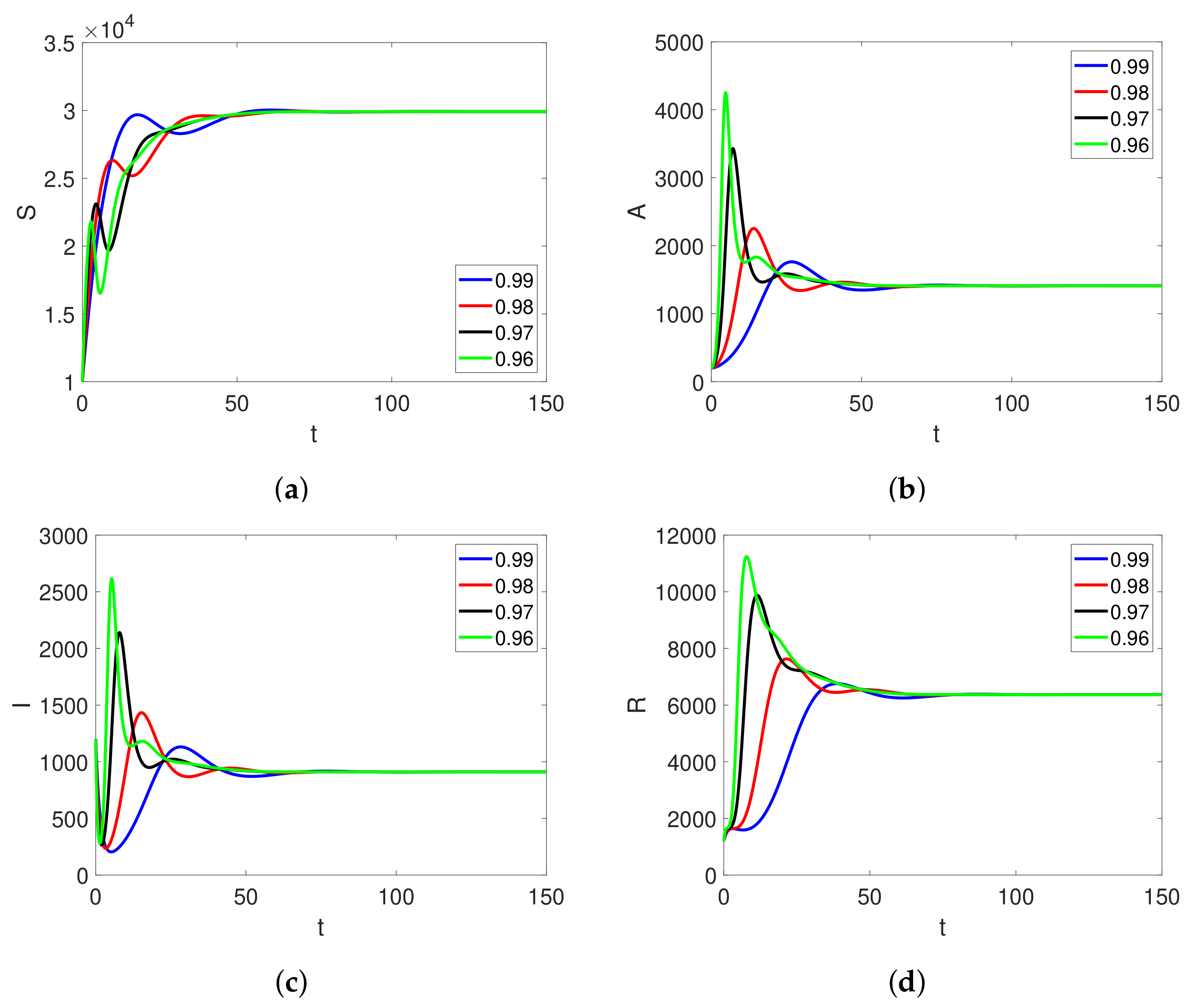
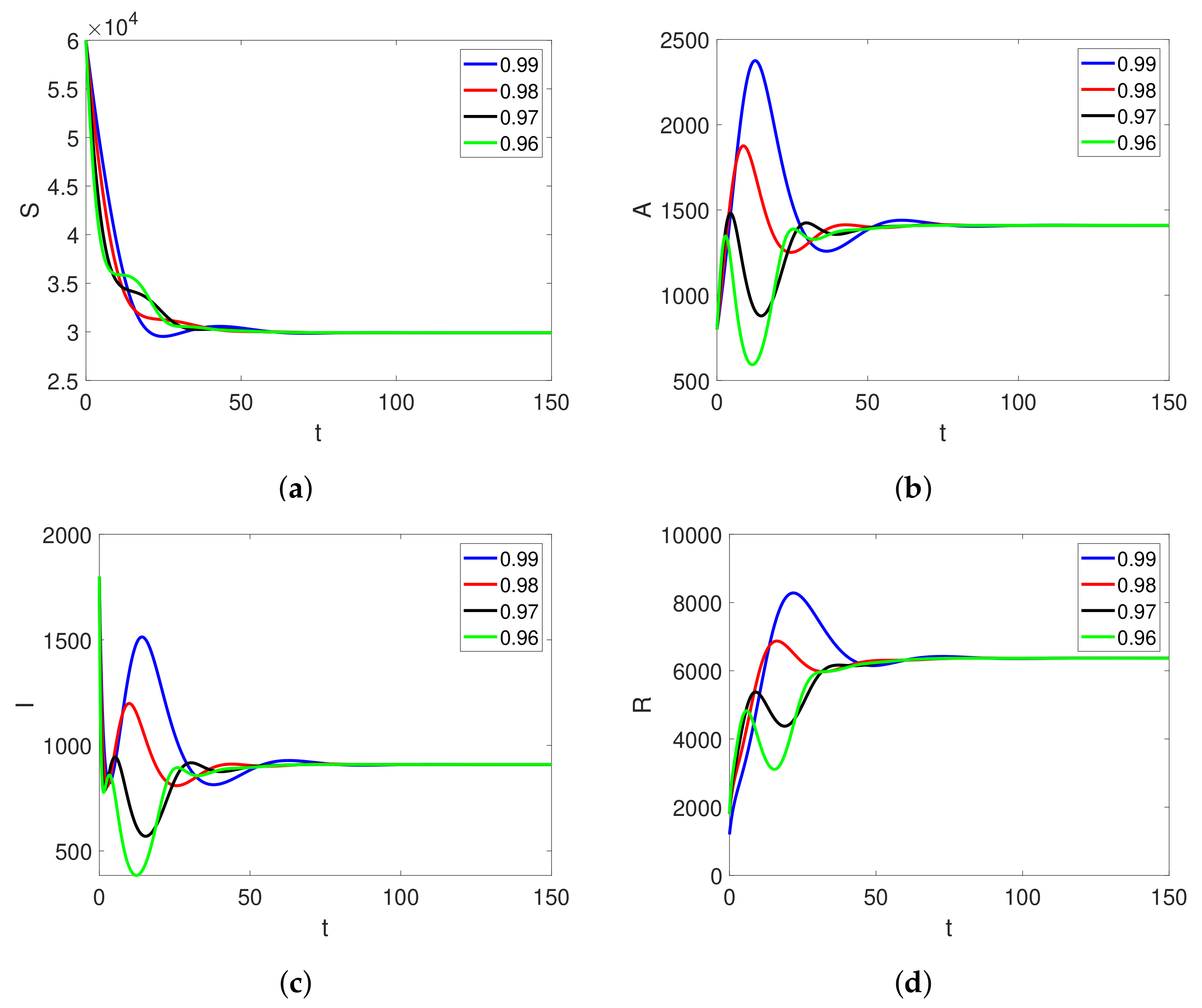
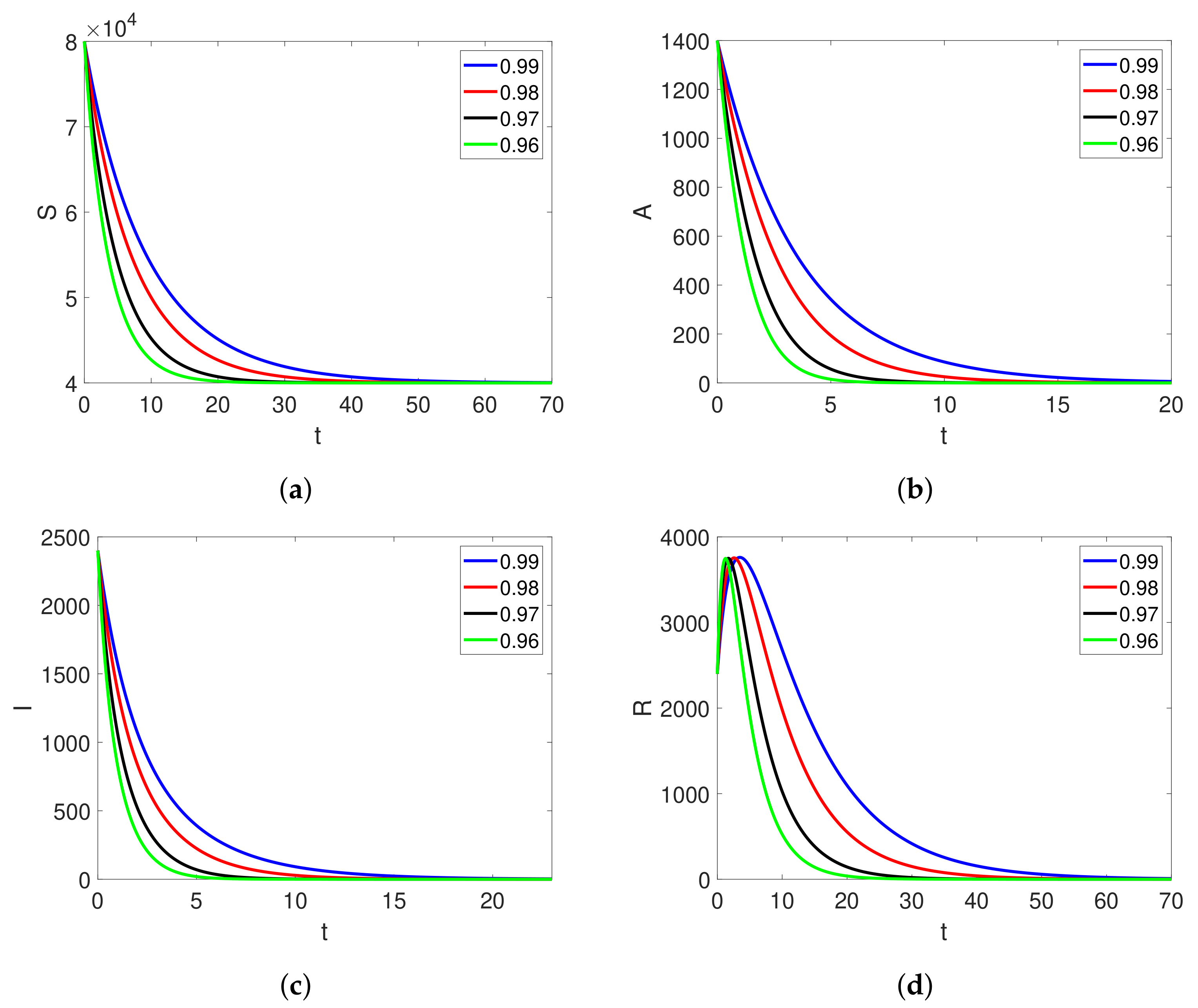
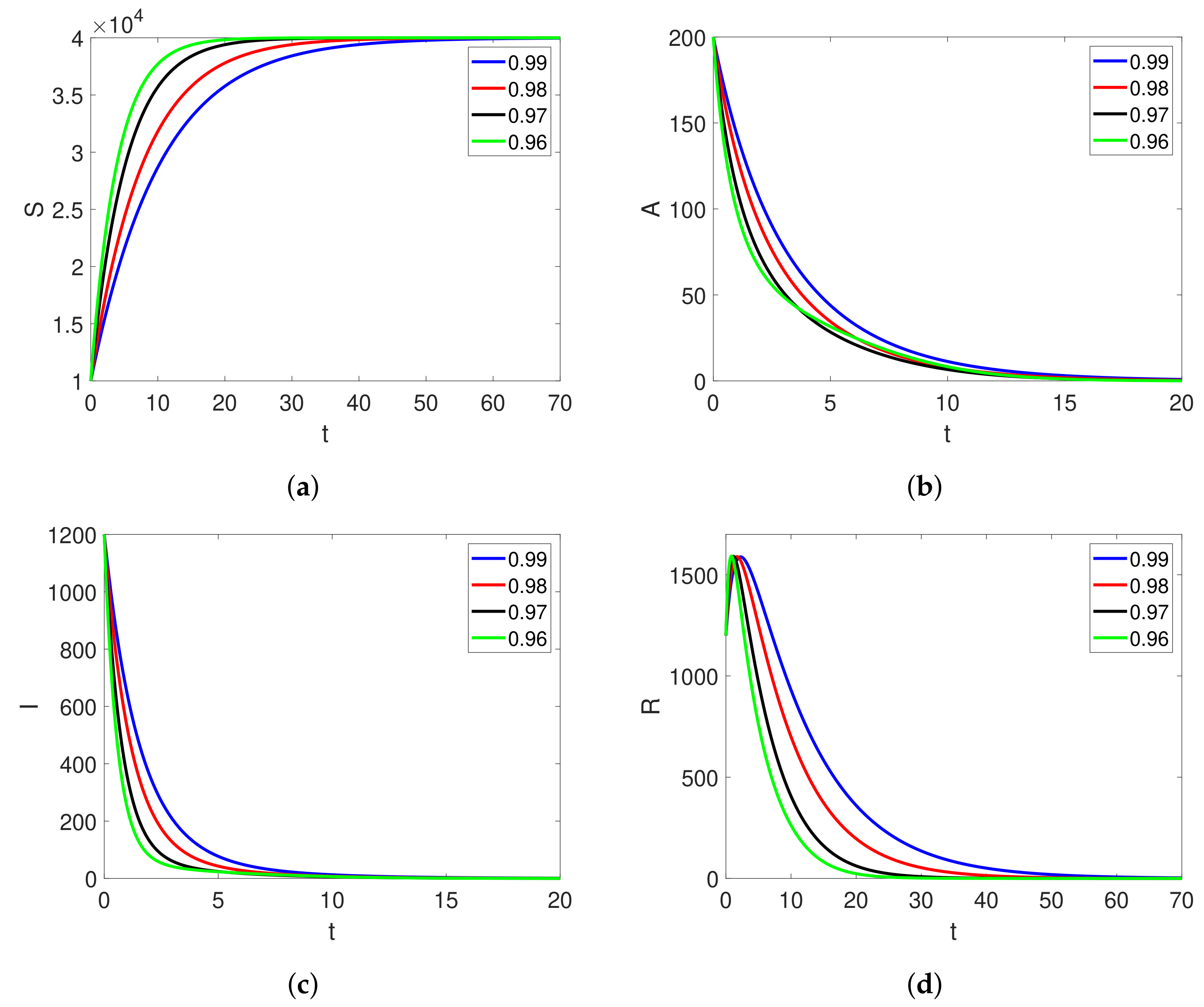
The purpose of this section is to provide the simulations of the results obtained in the above section via the Newton polynomial interpolation scheme. The values of the parameters present in the suggested system were considered in two different sets, as presented in

Table 1. The parameters and their values for model (2).

Parameters	Set 1	Set 2
$\Pi$	2600	2600
⋏	0.6	0.3
$\upsilon$	0.065	0.065
$q_1$	0.3	0.3
$q_2$	0.1	0.1
$\kappa$	0.3	0.3
$\nu$	0.1	0.1

. The parameters in set 1 were used for Figure 1, Figure 2 and Figure 3, while the parameter values of set 2 were used for Figure 4, Figure 5 and Figure 6. The initial values were considered in three different sets. The initial conditions in set 1 were $\mathsf{S}=8000$, $\mathsf{A}=1400$, $\mathsf{I}=2400$, and $\mathsf{R}=2400$; in set 2, they were $\mathsf{S}=10000$, $\mathsf{A}=200$, $\mathsf{I}=1200$, and $\mathsf{R}=1200$, and in set 3, the initial conditions were considered as $\mathsf{S}$ = 60,000, $\mathsf{A}=800$, $\mathsf{I}=1800$, and $\mathsf{R}=1800$. In the figures, the initial values of set 1 were used in Figure 1 and Figure 4, that of set 2 were used in Figure 2 and Figure 5, and finally the values of set 3 were used in Figure 3 and Figure 6.

In Figure 1a, Figure 2a, Figure 3a, Figure 4a, Figure 5a, Figure 6a, the population behavior of the susceptible population is presented. We see in Figure 1a, Figure 2a, Figure 3a that when the value of ⋏ was large, there were oscillations in the behavior, which moved towards stability when $t=60$. Further, Figure 1b, Figure 2b, Figure 3b, Figure 4b, Figure 5b, Figure 6b show the dynamics of the asymptomatic individuals, where it can be seen that the asymptomatic population increased as the time passed, while the individuals in this class became constant as $t=70$ at lower fractional orders. Similarly, Figure 1c, Figure 2c, Figure 3c, Figure 4c, Figure 5c, Figure 6c and Figure 1d, Figure 2d, Figure 3d, Figure 4d, Figure 5d, Figure 6d show the population dynamics in the infected and recovered individuals, respectively. From Figure 1c and Figure 2c, we observed that the infected population increased at the beginning, which showed a decrease as the time passed, while a fast decrease was observed in the infected population in Figure 3c, when the fractional order was $0.96$. Further, the recovered population kept increasing and then became stable at $t=60$, it was also observed that the recovered population was very large when compared to the those infected with the virus.

Figure 4, Figure 5 and Figure 6 are projected to show the dynamics in various state variables where the basic reproductive number was less than zero or where the disease died out. For this purpose, we considered the parameter $⋏=0.3$. Here, the fractional orders were considered to be $(blue,0.99),(red,0.98),(black,0.97)$, and $(green,0.96)$. From all of the following, we see that the state variables became stable at lower fractional orders as compared to the high orders.

7. Conclusions

In this article, we studied the fractional order COVID-19 ($\mathsf{SAIR}$) model in the sense of a Caputo operator. This model had a nonlinear incidence rate, constant input rate, and constant treatment rate. The existence and uniqueness of the associated solution was studied through the tools from fixed point theory. Numerically, the solution of the model was approximated with the Newton Polynomial interpolation scheme. Simulations of the results were presented, where it was observed that when the value of ⋏ was large, there were oscillations in the behaviors of the state variables, which moved toward stability faster at lower fractional orders. Similarly, the recovered population was observed to be increasing as time passed and then became stable at $t=60$; we also observed that the recovered population was very large as compared to those who were infected with the virus.

References

1. Poutanen, S.M.; Low, D.E.; Henry, B.; Finkelstein, S.; Rose, D.; Green, K.; Tellier, R.; Draker, R.; Adachi, D.; Ayers, M.; et al. Identification of severe acute respiratory syndrome in Canada. N. Engl. J. Med. 2003, 348, 1995–2005. [Google Scholar] [CrossRef] [PubMed]
2. De Groot, R.J.; Baker, S.C.; Baric, R.S.; Brown, C.S.; Drosten, C.; Enjuanes, L.; Fouchier, R.A.M.; Galiano, M.; Gorbalenya, A.E.; Memish, Z.A.; et al. Commentary: Middle east respiratory syndrome coronavirus (mers-cov): Announcement of the coronavirus study group. J. Virol. 2013, 87, 7790–7792. [Google Scholar] [CrossRef] [PubMed] [Green Version]
3. Read, J.M.; Bridgen, J.R.; Cummings, D.A.; Ho, A.; Jewell, C.P. Novel coronavirus 2019-nCoV: Early estimation of epidemiological parameters and epidemic predictions. medRxiv 2020. [Google Scholar] [CrossRef] [Green Version]
4. Shen, M.; Peng, Z.; Xiao, Y.; Zhang, L. Modeling the epidemic trend of the 2019 novel coronavirus outbreak in China. Innovation 2020, 1, 100048. [Google Scholar] [CrossRef]
5. Yu, Z.; Zhang, G.; Liu, Q.; Lv, Q. The outbreak assessment and prediction of 2019-nCoV based on time-varying SIR model. J. Univ. Electron. Sci. Technol. China 2020, 49, 357–361. [Google Scholar]
6. Asamoah, J.K.K.; Owusu, M.A.; Jin, Z.; Oduro, F.T.; Abidemi, A.; Gyasi, E.O. Global stability and cost-effectiveness analysis of COVID-19 considering the impact of the environment: Using data from Ghana. Chaos Solitons Fractals 2020, 140, 110103. [Google Scholar] [CrossRef]
7. Qian, M.; Jiang, J. COVID-19 and social distancing. J. Public Health 2022, 30, 259–261. [Google Scholar] [CrossRef]
8. Mwalili, S.; Kimathi, M.; Ojiambo, V.; Gathungu, D.; Mbogo, R. SEIR model for COVID-19 dynamics incorporating the environment and social distancing. BMC Res. Notes 2020, 13, 352. [Google Scholar] [CrossRef]
9. Elgazzar, A.S. Simple mathematical models for controlling COVID-19 transmission through social distancing and community awareness. Z. Naturforschung C 2021, 76, 393–400. [Google Scholar] [CrossRef]
10. Gao, W.; Veeresha, P.; Prakasha, D.G.; Baskonus, H.M. Novel dynamic structures of 2019-nCoV with nonlocal operator via powerful computational technique. Biology 2020, 9, 107. [Google Scholar] [CrossRef]
11. Mandal, M.; Jana, S.; Nandi, S.K.; Khatua, A.; Adak, S.; Kar, T.K. A model based study on the dynamics of COVID-19: Prediction and control. Chaos Solitons Fractals 2020, 136, 109889. [Google Scholar] [CrossRef] [PubMed]
12. Khan, M.A.; Atangana, A.; Alzahrani, E. The dynamics of COVID-19 with quarantined and isolation. Adv. Differ. Equ. 2020, 2020, 425. [Google Scholar] [CrossRef] [PubMed]
13. Ndaïrou, F.; Area, I.; Nieto, J.J.; Torres, D.F.M. Mathematical modeling of COVID-19 transmission dynamics with a case study of Wuhan. Chaos Solitons Fractals 2020, 135, 109846. [Google Scholar] [CrossRef] [PubMed]
14. Li, R.; Pei, S.; Chen, B.; Song, Y.; Zhang, T.; Yang, W.; Shaman, J. Substantial undocumented infection facilitates the rapid dissemination of novel coronavirus (SARS-CoV-2). Science 2020, 368, 489–493. [Google Scholar] [CrossRef] [Green Version]
15. Cai, J.; Sun, W.; Huang, J.; Gamber, M.; Wu, J.; He, G. Indirect virus transmission in cluster of COVID-19 cases, Wenzhou, China, 2020. Emerg. Infect. Dis. 2020, 26, 1343. [Google Scholar] [CrossRef]
16. Kang, X.; Hu, Y.; Liu, Z.; Sarwar, S. Forecast and evaluation of asymptomatic COVID-19 patients spreading in China. Results Phys. 2022, 34, 105195. [Google Scholar] [CrossRef]
17. Xu, C.; Saifullah, S.; Ali, A. Theoretical and numerical aspects of Rubella disease model involving fractal fractional exponential decay kernel. Results Phys. 2022, 34, 105287. [Google Scholar] [CrossRef]
18. Haidong, Q.; ur Rahman, M.; Arfan, M. Fractional model of smoking with relapse and harmonic mean type incidence rate under Caputo operator. J. Appl. Math. Comput. 2022, 1–18. [Google Scholar] [CrossRef]
19. Atangana, A.; Baleanu, D. New fractional derivatives with nonlocal and non-singular kernel: Theory and application to heat transfer model. arXiv 2016, arXiv:1602.03408. [Google Scholar] [CrossRef] [Green Version]
20. Podlubny, I. An introduction to fractional derivatives, fractional differential equations, to methods of their solution and some of their applications. Math. Sci. Eng. 1999, 198, 340. [Google Scholar]
21. Zhang, L.; ur Rahman, M.; Arfan, M.; Ali, A. Investigation of mathematical model of transmission co-infection TB in HIV community with a non-singular kernel. Results Phys. 2021, 28, 104559. [Google Scholar] [CrossRef]
22. Shen, W.-Y.; Chu, Y.-M.; ur Rahman, M.; Mahariq, I.; Zeb, A. Mathematical analysis of HBV and HCV co-infection model under nonsingular fractional order derivative. Results Phys. 2021, 28, 104582. [Google Scholar] [CrossRef]
23. Xu, C.; ur Rahman, M.; Baleanu, D. On fractional-order symmetric oscillator with offset-boosting control. Nonlinear Anal. Model. Control 2022, 27, 994–1008. [Google Scholar] [CrossRef]
24. Saifullah, S.; Ali, A.; Khan, Z.A. Analysis of nonlinear time-fractional Klein-Gordon equation with power law kernel. AIMS Math. 2022, 7, 5275–5290. [Google Scholar] [CrossRef]
25. Khan, Z.A.; Khan, J.; Saifullah, S.; Ali, A. Dynamics of Hidden Attractors in Four-Dimensional Dynamical Systems with Power Law. J. Funct. Spaces 2022, 2022, 3675076. [Google Scholar] [CrossRef]
26. Alqahtani, R.T.; Ahmad, S.; Akgül, A. Dynamical analysis of bio-ethanol production model under generalized nonlocal operator in Caputo sense. Mathematics 2021, 9, 2370. [Google Scholar] [CrossRef]
27. Jain, S. Numerical analysis for the fractional diffusion and fractional Buckmaster equation by the two-step Laplace Adam-Bashforth method. Eur. Phys. J. Plus 2018, 133, 19. [Google Scholar] [CrossRef]
28. Atangana, A.; Jain, S. A new numerical approximation of the fractal ordinary differential equation. Eur. Phys. J. Plus 2018, 133, 37. [Google Scholar] [CrossRef]
29. Saifullah, S.; Ali, A.; Irfan, M.; Shah, K. Time-fractional Klein–Gordon equation with solitary/shock waves solutions. Math. Probl. Eng. 2021, 2021, 6858592. [Google Scholar] [CrossRef]
30. Araz, S.İ. Analysis of a COVID-19 model: Optimal control, stability and simulations. Alex. Eng. J. 2021, 60, 647–658. [Google Scholar] [CrossRef]
31. Awais, M.; Alshammari, F.S.; Ullah, S.; Khan, M.A.; Islam, S. Modeling and simulation of the novel coronavirus in Caputo derivative. Results Phys. 2020, 19, 103588. [Google Scholar] [CrossRef] [PubMed]
32. Ullah, S.; Khan, M.A. Modeling the impact of non-pharmaceutical interventions on the dynamics of novel coronavirus with optimal control analysis with a case study. Chaos Solitons Fractals 2020, 139, 110075. [Google Scholar] [CrossRef] [PubMed]
33. Li, B.; Liang, H.; He, Q. Multiple and generic bifurcation analysis of a discrete Hindmarsh-Rose model. Chaos Solitons Fractals 2021, 146, 110856. [Google Scholar] [CrossRef]
34. Li, B.; Liang, H.; Shi, L.; He, Q. Complex dynamics of Kopel model with nonsymmetric response between oligopolists. Chaos Solitons Fractals 2022, 156, 111860. [Google Scholar] [CrossRef]
35. Eskandari, Z.; Avazzadeh, Z.; Ghaziani, R.K.; Li, B. Dynamics and bifurcations of a discrete-time Lotka–Volterra model using nonstandard finite difference discretization method. Math. Methods Appl. Sci. 2022. [Google Scholar] [CrossRef]
36. Baleanu, D.; Abadi, M.H.; Jajarmi, A.; Vahid, K.Z.; Nieto, J.J. A new comparative study on the general fractional model of COVID-19 with isolation and quarantine effects. Alex. Eng. J. 2022, 61, 4779–4791. [Google Scholar] [CrossRef]
37. Zhang, L.; Addai, E.; Ackora-Prah, J.; Arthur, Y.D.; Asamoah, J.K.K. Fractional-Order Ebola-Malaria Coinfection Model with a Focus on Detection and Treatment Rate. Comput. Math. Methods Med. 2022, 2022, 6502598. [Google Scholar] [CrossRef]
38. Gómez-Aguilar, J.F.; Rosales-García, J.J.; Bernal-Alvarado, J.J.; Córdova-Fraga, T.; Guzmán-Cabrera, R. Fractional mechanical oscillators. Rev. Mex. Física 2012, 58, 348–352. [Google Scholar]
39. Afshari, H.; Hosseinpour, H.; Marasi, H.R. Application of some new contractions for existence and uniqueness of differential equations involving Caputo–Fabrizio derivative. Adv. Differ. Equ. 2021, 2021, 321. [Google Scholar] [CrossRef]
40. Ulam, S.M. A Collection of Mathematical Problems; Interscience Publishers: New York, NY, USA, 1960; p. 29. [Google Scholar]
41. Ulam, S.M. Problem in Modren Mathematics; Courier Corporation: Mineola, NY, USA, 2004. [Google Scholar]
Figure 1. The dynamics of the state variables’ SAIR in model (2) with different fractional orders α vs. time t with initial conditions.
Fractalfract 07 00046 g001
Figure 2. The dynamics of the state variables’ SAIR in model (2) with different fractional orders α vs. time t with initial conditions.
Fractalfract 07 00046 g002
Figure 3. The dynamics of the state variables’ SAIR in model (2) with different fractional orders α vs. time t with initial conditions.
Fractalfract 07 00046 g003
Figure 4. The dynamics of the state variables’ SAIR in model (2) with different fractional orders α vs. time t with initial conditions.
Fractalfract 07 00046 g004
Figure 5. The dynamics of the state variables’ SAIR in model (2) with different fractional orders α vs. time t with initial conditions.
Fractalfract 07 00046 g005
Figure 6. The dynamics of the state variables’ SAIR in model (2) with different fractional orders α vs. time t with initial conditions.
Fractalfract 07 00046 g006