Article

Investigation of Novel Piecewise Fractional Mathematical Model for COVID-19

by
Ibtehal Alazman
1 and
Badr Saad T. Alkahtani
2,*
1
Department of Mathematics and Statistics, College of Science, Imam Mohammad Ibn Saud Islamic University (IMSIU), Riyadh 11566, Saudi Arabia
2
Department of Mathematics, College of Science, King Saud University, Riyadh 11989, Saudi Arabia
*
Author to whom correspondence should be addressed.
Fractal Fract. 2022, 6(11), 661; https://doi.org/10.3390/fractalfract6110661
Submission received: 12 September 2022 / Revised: 27 October 2022 / Accepted: 31 October 2022 / Published: 9 November 2022
(This article belongs to the Special Issue Fractal Approaches in Materials: Structure and Mechanics)

Abstract

:
The outbreak of coronavirus (COVID-19) began in Wuhan, China, and spread all around the globe. For analysis of the said outbreak, mathematical formulations are important techniques that are used for the stability and predictions of infectious diseases. In the given article, a novel mathematical system of differential equations is considered under the piecewise fractional operator of Caputo and Atangana–Baleanu. The system is composed of six ordinary differential equations (ODEs) for different agents. The given model investigated the transferring chain by taking non-constant rates of transmission to satisfy the feasibility assumption of the biological environment. There are many mathematical models proposed by many scientists. The existence of a solution along with the uniqueness of a solution in the format of a piecewise Caputo operator is also developed. The numerical technique of the Newton interpolation method is developed for the piecewise subinterval approximate solution for each quantity in the sense of Caputo and Atangana-Baleanu-Caputo (ABC) fractional derivatives. The numerical simulation is drawn against the available data of Pakistan on three different time intervals, and fractional orders converge to the classical integer orders, which again converge to their equilibrium points. The piecewise fractional format in the form of a mathematical model is investigated for the novel COVID-19 model, showing the crossover dynamics. Stability and convergence are achieved on small fractional orders in less time as compared to classical orders.

1. Introduction

An outbreak of coronavirus spread from Wuhan city and affected people all over the world. Coronavirus is a virus that is responsible for a respiratory infectious disease. The World Health Organization (WHO) named this virus COVID-19, as it was tested for the first time in December 2019. In the first phase, 55% of infected people were linked to the human seafood market after spreading from person to person [1]. This pandemic first spread into China and then all over the globe. After several weeks, this novel coronavirus became a global concern for humans.
Mathematicians started working on this new disease to control it by using optimal control strategies in mathematical models. Simulations and the modeling of infectious diseases play an important role in discussing the phenomena of controlling infectious diseases in human and animal populations [2,3,4]. In the early 2020s, several researchers published work on this pandemic, such as those given in [5,6,7,8]. From all over the world, several research articles have been published on the spread of COVID-19, which have been very useful for understanding the virus infection [9,10,11,12]. In the existing literature, a classical model called SIR (susceptible–infectious–removed) is used for modeling infectious diseases. Several researchers have used the idea of SIR and further modified it by adding other compartments and studying different aspects, which can be seen [13,14,15,16]. Many researchers have investigated the novel virus by adding isolation and quarantine classes to reduce the spread of the disease [17,18].
As far as the novelty and motivation of the paper are concerned, a novel mathematical system of differential equations is considered under the piecewise fractional operator of Caputo and Atangana–Baleanu, which describes the crossover dynamics of COVID-19. The existence of a solution along with the uniqueness of a solution in the format of piecewise Caputo and ABC operators is also developed. The predictor and corrector methods of the Adams–Bashforth method are developed for the piecewise subinterval approximate solution for each quantity. The numerical simulation is drawn against the available data of Pakistan on three different time durations and fractional orders converging to the integer orders.
In this manuscript, a newly constructed model is proposed [19]. The effects of government action, conditions, and personal reactions are also included. In the newly constructed model, the total populace is divided into six sub-classes, including susceptible S , class of exposed E , class of infected I , class of quarantined Q , class of recovered R and isolated class G . This study also included the rate of transmission from person to person. Following government action, we included the isolation of humans. The system of ordinary differential equations in the considered article is as follows:
S ˙ ( t ) = Λ α E S E α I S I δ S μ S , E ˙ ( t ) = α E S E + α I S I β E μ E , I ˙ ( t ) = β E γ I μ I , Q ˙ ( t ) = γ I ( r + d ) Q μ Q , R ˙ ( t ) = ( r + d ) Q μ R , G ˙ ( t ) = δ S μ G ,
with initial conditions
S ( 0 ) = S 0 , E ( 0 ) = E 0 , I ( 0 ) = I 0 , Q ( 0 ) = Q 0 , R ( 0 ) = R 0 , G ( 0 ) = G 0 .
The parameters of the above model are defined as follows: Λ represents the birth rate, α E represents the rate of transmission from person to person of the class S , α I also represents the rate of transmission from person to person of the class I , the rate of natural death is represented by μ , β represents the average latent time, and γ represents the average quarantine time. The parameter δ represents the rate of protection, while r and d represent the rate of cure and mortality.
For the analysis of crossover problems, different operators are introduced, including fractal derivative, non-integer order derivative with a kernel of singularity and non-singularity, fractional-fractal operator, and some other derivative operators; see [20,21,22,23,24]. The inclusion of randomness in the form of the stochastic equation has more realistic achievements, but still, the crossover dynamics are not solved. This property is found in many infectious disease models, the flow of heat, fluid flow, and many complex advection problems [24,25,26]. In fractional calculus, the exponential and Mittag–Leffler mappings are not able to find the time of crossovers. Therefore, to solve such problems, one of the new approaches to piece-wise differentiation and integration is introduced in [27]. They introduced the classical and global piecewise derivatives along with some application examples. We will investigate the said problem for qualitative analysis, numerical iterative analysis, and stability analysis in the sense of the Caputo and Atangana–Baleanu piecewise derivative. The considered system (1) can be written in the aforementioned derivative, which is defined as
CABC D t ς ( S ( t ) ) = Λ α E S E α I S I δ S μ S , CABC D t ς ( E ( t ) ) = α E S E + α I S I β E μ E , CABC D t ς ( I ( t ) ) = β E γ I μ I , CABC D t ς ( Q ( t ) ) = γ I ( r + d ) Q μ Q , CABC D t ς ( R ( t ) ) = ( r + d ) Q μ R , CABC D t ς ( G ( t ) ) = δ S μ G , S ( 0 ) = S 0 , E ( 0 ) = E 0 , I ( 0 ) = I 0 , Q ( 0 ) = Q 0 , R ( 0 ) = R 0 , G ( 0 ) = G 0 .
In more detail, we can write Equation (2) as
0 CABC D t ς ( S ( t ) ) = 0 C D t ς ( S ( t ) ) = C 1 ( S , t ) , 0 < t t 1 , 0 ABC D t ς ( S ( t ) ) = ABC 1 ( S , t ) , t 1 < t T , 0 CABC D t ς ( E ( t ) ) = 0 C D t ς ( E ( t ) ) = C 2 ( R , t ) , 0 < t t 1 , 0 ABC D t ς ( E ( t ) ) = ABC 2 ( E , t ) , t 1 < t T , 0 CABC D t ς ( I ( t ) ) = 0 C D t ς ( I ( t ) ) = C 3 ( I , t ) , 0 < t t 1 , 0 ABC D t ς ( I ( t ) ) = ABC 3 ( I , t ) , t 1 < t T , 0 CABC D t ς ( Q ( t ) ) = 0 C D t ς ( Q ( t ) ) = C 4 ( Q , t ) , 0 < t t 1 , 0 ABC D t ς ( Q ( t ) ) = ABC 4 ( Q , t ) , t 1 < t T , 0 CABC D t ς ( R ( t ) ) = 0 C D t ς ( R ( t ) ) = C 5 ( R , t ) , 0 < t t 1 , 0 ABC D t ς ( R ( t ) ) = ABC 5 ( R , t ) , t 1 < t T , 0 CABC D t ς ( G ( t ) ) = 0 C D t ς ( G ( t ) ) = C 6 ( G , t ) , 0 < t t 1 , 0 ABC D t ς ( G ( t ) ) = ABC 6 ( G , t ) , t 1 < t T ,
where 0 C D t ς and 0 ABC D t ς represent the Caputo and A B C derivatives respectively.
This paper is organized as follows: Section 2 includes the basic results of fractional and piecewise differentials and integrals from the literature. In Section 3, we show the existence results, uniqueness of the solution and Ulam–Hyers stability for the considered model. In Section 4, using the piecewise differential and integral technique, we find the approximate solution for the model. In Section 5, we discuss the obtained results graphically and compare the used method with the Laplace Adomian decomposition method. Finally, we conclude our work in Section 6.

2. Preliminaries

This part is devoted to some preliminary definitions of Caputo and ABC fractional derivatives and integrals.
Definition 1
([20]). Considering a function Y ( t ) with condition Y ( t ) I 1 ( 0 , T ) , the ABC derivative is given as
ABC 0 D t ς ( Y ( t ) ) = M ( ς ) 1 ς 0 t d d ξ Y ( ξ ) E ς ς 1 ς t ξ ς d ξ .
Replace E ς ς 1 ς t ξ ξ by E 1 = exp r 1 ς t ξ , in (4), and we will obtain the Caputo–Fabrizio operator. Next, it is notified that
ABC 0 D t ς [ c o n s t a n t ] = 0 .
Here, M ( ς ) is known as the normalization function and M ( 0 ) = M ( 1 ) = 1 . Further, E ς shows the Mittag–Leffler (ML) function, and is known as the generalization of the exponential function [28,29,30].
The integration in the sense of A B C is given as
ABC 0 I t ς Y ( t ) = 1 ς M ( ς ) Y ( t ) + ς M ( ς ) Γ ( ς ) 0 t ( t ξ ) ς 1 Y ( ξ ) d ξ .
Definition 2
([31]). The Caputo derivative for a function Y ( t ) is defined as
0 C D t ς Y ( t ) = 1 Γ ( 1 ς ) 0 t ( t ξ ) n ς 1 [ Y ( ξ ) ] d ξ .
Definition 3
([27]). The classical piecewise derivative for a function Y ( t ) and g ( t ) which is differentiable and increasing is defined as
0 P G D t Y ( t ) = Y ( t ) , 0 < t t 1 , Y ( t ) g ( t ) t 1 < t T ,
where 0 P G D t Y ( t ) represents the classical derivative for 0 < t t 1 and global derivative for t 1 < t T .
The integration for classical piecewise is defined as
0 P G I t Y ( t ) = 0 t Y ( τ ) d τ , 0 < t t 1 , t 1 t Y ( τ ) g ( τ ) d ( τ ) t 1 < t T ,
where 0 P G I t Y ( t ) represents the classical integration for 0 < t t 1 and global integration for t 1 < t T .
Definition 4
([27]). The classical and fractional piecewise derivative for a function Y ( t ) is defined as
0 P C D t ς Y ( t ) = Y ( t ) , 0 < t t 1 , 0 C D t ς Y ( t ) t 1 < t T ,
where 0 P C D t ς Y ( t ) represents the classical derivative 0 < t t 1 and fractional derivative t 1 < t T .
The integration for classical and fractional piecewise derivatives is given as
0 P C I t Y ( t ) = 0 t Y ( τ ) d τ , 0 < t t 1 , 1 Γ r t 1 t ( t ξ ) ς 1 Y ( ξ ) d ( ξ ) t 1 < t T ,
where 0 P C I t Y ( t ) represents the classical, 0 < t t 1 and Caputo integration t 1 < t T .
Definition 5
([27]). The fractional piecewise derivative for a differentiable function Y ( t ) in the sense of Caputo, and ABC is represented as
0 P C ABC D t ς Y ( t ) = 0 C D t ς Y ( t ) , 0 < t t 1 , 0 ABC D t ς Y ( t ) t 1 < t T ,
where 0 P C ABC D t ς Y ( t ) represent the Caputo, 0 < t t 1 and ABC derivative t 1 < t T .
The integration is defined as
0 P C ABC I t Y ( t ) = 1 Γ ( ς ) t 1 t ( t ξ ) ς 1 Y ( ξ ) d ( ξ ) , 0 < t t 1 , 1 ς M ( ς ) Y ( t ) + ς M ( ς ) Γ ( ς ) t 1 t ( t ξ ) ς 1 Y ( ξ ) d ( ξ ) t 1 < t T ,
where 0 P C ABC I t Y ( t ) represent the Caputo, 0 < t t 1 and ABC integration t 1 < t T .
Lemma 1
([32,33,34,35]). The solution of piecewise derivable equations
0 P C D t 1 ς K ( t ) = H ( t , K ( t ) ) , t [ 0 , t 1 ] 0 < ς 1 K ( 0 ) = K 0 , K t 1 PABC D t ς K ( t ) = H ( t , K ( t ) ) , t [ t 1 , T ] 0 < ς 1 K ( t 1 ) = K t 1 ,
is
K ( t ) = K 0 + 1 Γ ( ς ) 0 t 1 H ( ξ , K ( ξ ) ) ( t ξ ) ς 1 d ξ , 0 < t t 1 K ( t 1 ) + 1 ς M ( ς ) H ( t , K ( t ) ) + ς M ( ς ) Γ ( ς ) t 1 t ( t ξ ) ς 1 H ( ξ K ( ξ ) ) d ( ξ ) t 1 < t T
Proof. 
For the proof, we apply the piecewise Caputo (PC) integral and (PABC) integral on each interval to the above equation as
0 P C I t 1 ς P C 0 D t 1 ς K ( t ) = 0 P C I t 1 ς H ( t , K ( t ) ) , t [ 0 , t 1 ] 0 < ς 1 t 1 PABC I t ς PABC t 1 D t ς K ( t ) = t 1 PABC I t ς H ( t , K ( t ) ) , t [ t 1 , T ] 0 < ς 1 ,
and using the initial conditions, we obtain
K ( t ) K ( 0 ) = 1 Γ ( ς ) 0 t 1 H ( ξ , K ( ξ ) ) ( t ξ ) ς 1 d ξ , 0 < t t 1 K ( t ) K ( t 1 ) = 1 ς M ( ς ) H ( t , K ( t ) ) + ς M ( ς ) Γ ( ς ) t 1 t ( t ξ ) ς 1 H ( ξ K ( ξ ) ) d ( ξ ) t 1 < t T ,
which further implies
K ( t ) = K ( 0 ) + 1 Γ ( ς ) 0 t 1 H ( ξ , K ( ξ ) ) ( t ξ ) ς 1 d ξ , 0 < t t 1 K ( t 1 ) + 1 ς M ( ς ) H ( t , K ( t ) ) + ς M ( ς ) Γ ( ς ) t 1 t ( t ξ ) ς 1 H ( ξ K ( ξ ) ) d ( ξ ) t 1 < t T
Hence, it is proved. □

3. Piecewise Existence and Uniqueness of Solution

Next, we find the existence results and uniqueness of the solution property of the considered piecewise derivable problem. For this, we use Lemma 1 and rewrite model (3) as
0 P CABC D t ς K ( t ) = F ( t , K ( t ) ) , 0 < r 1
is
K ( t ) = K 0 + 1 Γ ( ς ) 0 t F ( ξ , K ( ξ ) ) ( t ξ ) ς 1 d ξ , 0 < t t 1 K ( t 1 ) + 1 ς M ( ς ) F ( t , K ( t ) ) + ς M ( ς ) Γ r t 1 t ( t ξ ) ς 1 F ( ξ K ( ξ ) ) d ( ξ ) , t 1 < t T ,
where
K ( t ) = S ( t ) E ( t ) I ( t ) Q ( t ) R ( t ) G ( t ) , K 0 = S 0 E 0 I 0 Q 0 R 0 G 0 , K ( t 1 ) = S ( t 1 ) E ( t 1 ) I ( t 1 ) Q ( t 1 ) R ( t 1 ) G ( t 1 ) , F ( t , K ( t ) ) = 1 = C 1 ( S , t ) ABC 1 ( S , t ) F 2 = C 2 ( E , t ) ABC 2 ( E , t ) F 3 = C 3 ( I , t ) ABC 3 ( I , t ) F 4 = C 4 ( Q , t ) ABC 4 ( Q , t ) F 5 = C 5 ( R , t ) ABC 5 ( R , t ) F 6 = C 6 ( G , t ) ABC 6 ( G , t ) ,
By choosing > T t > 0 with a Banach space, A 1 = ( C [ 0 , T ] × R 6 , R + ) . Further, M = A 1 × A 2 × A 3 × A 4 × A 5 × A 6 is also a complete norm space endowed with the norm, having the norm
K = max t [ 0 , T ] | K ( t ) | = sup t [ 0 , T ] [ | S ( t ) | + | E ( t ) | + | I ( t ) | + | Q ( t ) | + | R ( t ) | + | G ( t ) | ] ,
which can be written as in Equation (6).
To obtain the required result, we take the growth condition on a non-linear operator as
(C1) 
L K > 0 ; ∀ F , K ¯ E we have
| F ( t , K ) H ( t , K ¯ ) | L F | K K ¯ | ,
(C2) 
C F > 0 & M F > 0 ;
| F ( t , K ( t ) ) | C F | K | + M F .
Theorem 1.
If F is a piecewise continuous operator on sub interval 0 < t t 1 and t 1 < t T on [ 0 , T ] , also obeying ( C 2 ) , then piecewise problem (3) has at least one solution on each sub interval.
Proof. 
By applying the Schauder fixed-point theorem, let us define a closed subset in both the subinterval of 0 , T as B of E as
B = { K E : K R 1 , 2 , R > 0 } ,
Next, we take an operator T : B B , and applying (6) as
T ( K ) = K 0 + 1 Γ ( ς ) 0 t 1 F ( ξ , K ( ξ ) ) ( t ξ ) ς 1 d ξ , 0 < t t 1 K ( t 1 ) + 1 ς M ( ς ) F ( t , K ( t ) ) + ς M ( ς ) Γ ( ς ) t 1 t ( t ξ ) ς 1 H ( ξ K ( ξ ) ) d ( ξ ) , t 1 < t T ,
On any K B , we obtain
| T ( K ) ( t ) | | K 0 | + 1 Γ ( ς ) 0 t 1 ( t ξ ) ς 1 | F ( ξ , K ( ξ ) ) | d ξ , | K t 1 | + 1 ς M ( ς ) | F ( t , K ( t ) ) | + ς M ( ς ) Γ ( ς ) t 1 t ( t ξ ) ς 1 | F ( ξ K ( ξ ) ) | d ( ξ ) , | K 0 | + 1 Γ ( ς ) 0 t 1 ( t ξ ) ς 1 [ C F | K | + M F ] d ξ , | K t 1 | + 1 ς M ( ς ) [ C F | K | + M F ] + ς M ( ς ) Γ ( ς ) t 1 t ( t ξ ) ς 1 [ C F | K | + M F ] d ( ξ ) , | K 0 | + T ς Γ ( ς + 1 ) [ C F | K | + M F ] = R 1 , 0 < t t 1 , | K t 1 | + 1 ς M ( ς ) [ C F | K | + M F ] + r ( T T ) ς M ( ς ) Γ r + 1 [ C F | K | + M F ] d ( ξ ) = R 2 , t 1 < t T , R 1 , 0 < t t 1 , R 2 , t 1 < t T .
from the last equation, as K B . Therefore, T ( B ) B . Thus, this proves that the operator T is complete and close. Next, for complete continuity, we take t i < t j [ 0 , t 1 ] as the first interval of the Caputo sense, and assume
| T ( K ) ( t j ) T ( K ) ( t i ) | = | 1 Γ ( ς ) 0 t j ( t j ξ ) ς 1 F ( ξ , K ( ξ ) ) d ξ , 1 Γ ( ς ) 0 t i ( t i ξ ) ς 1 F ( ξ , K ( ξ ) ) d ξ | 1 Γ ( ς ) 0 t i [ ( t i ξ ) ς 1 ( t j ξ ) ς 1 ] | F ( ξ , K ( ξ ) ) | d ξ + 1 Γ ( ς ) t i t j ( t j ξ ) ς 1 | F ( ξ , K ( ξ ) ) | d ξ 1 Γ ( ς ) [ 0 t i [ ( t i ξ ) ς 1 ( t j ξ ) ς 1 ] d ξ + t i t j ( t j ξ ) ς 1 d ξ ] ( C F | K | + M F ) ( C F K + M F ) Γ ( ς + 1 ) [ t j ς t i ς + 2 ( t j t i ) ς ] .
Next (9), we obtain t i t j , then
| T ( K ) ( t j ) T ( K ) ( t i ) | 0 , as t i t j .
So, T is equi-continuous in the [ 0 , t 1 ] interval. Next, we take the other interval t i , t j [ t 1 , T ] in the ABC sense as
| T ( K ) ( t j ) T ( K ) ( t i ) | = | 1 ς M ( ς ) F ( t , K ( t ) ) + ς M ( ς ) Γ ( ς ) t 1 t j ( t j ξ ) ς 1 F ( ξ , K ( ξ ) ) d ξ , 1 ς M ( ς ) F ( t , K ( t ) ) + ( ς ) M ( ς ) Γ ( ς ) t 1 t i ( t i ξ ) ς 1 F ( ξ , K ( ξ ) ) d ξ | ς M ( ς ) Γ ( ς ) t 1 t i [ ( t i ξ ) ς 1 ( t j ξ ) ς 1 ] | F ( ξ , K ( ξ ) ) | d ξ + ς M ( ς ) Γ ( ς ) t i t j ( t j ξ ) ς 1 | F ( ξ , K ( ξ ) ) | d ξ ς M ( ς ) Γ ( ς ) [ t 1 t i [ ( t i ξ ) ς 1 ( t j ξ ) ς 1 ] d ξ + t i t j ( t j ξ ) ς 1 d ξ ] ( C F | K | + M F ) r ( C F K + M F ) M ( ς ) Γ ( ς + 1 ) [ t j ς t i ς + 2 ( t j t i ) ς ] .
Next, as (10), we obtain t i t j , then
| T ( K ) ( t j ) T ( K ) ( t i ) | 0 , as t i t j .
So, T is equi-continuous in the [ t 1 , T ] interval. Therefore, T is equi-continuous mapping. Using the Arzelá–Ascoli theorem, operator T is completely continuous and thus, uniform continuous and has bounds. So, by Schauder’s fixed-point theorem, piecewise derivable problem (3) has at least one solution. □
Theorem 2.
With assumption ( C 1 ) , the proposed system has a unique root if T is a contraction operator.
Proof. 
As we took operator T : B B as the piecewise continuous, we take K and K ¯ B on [ 0 , t 1 ] in the Caputo sense as
T ( K ) T ( K ¯ ) = max t [ 0 , t 1 ] | 1 Γ ( ς ) 0 t ( t ξ ) ς 1 F ( ξ , K ( ξ ) ) d ξ 1 Γ ( ς ) 0 t ( t ξ ) ς 1 F ( ξ , K ¯ ( ξ ) ) d ξ | T ς Γ ( ς + 1 ) L F K K ¯ .
From (11), we have
T ( K ) T ( K ¯ ) T ς Γ ( ς + 1 ) L F K K ¯ .
So, the operator T is a contraction. Therefore, by using the Banach contraction theorem, the system has a unique solution in the given sub-intervals. Further, for other interval t [ t 1 , T ] in the sense of the fractional A B C derivative as
T ( K ) T ( K ¯ ) 1 ς M ( ς ) L F K K ¯ + r ( T T ς ) M ( ς ) Γ ( ς + 1 ) L F K K ¯ .
or
T ( K ) T ( K ¯ ) L H 1 ς M ( ς ) + ς ( T T ) ς M ( ς ) Γ ( ς + 1 ) K K ¯ .
Thus, the system proves again the contraction and gives a unique solution in the sub-interval. Therefore, by Equations (12) and (14), the piecewise derivable problem has a unique solution on every sub-interval. □

Stability Analysis

Here, we proved the Ulam–Hyers (H-U) stability and different forms for our considered model. First, we give some definitions related to (H-U).
Definition 6.
Our proposed model (2) is H-Ustable, if for each σ > 0 , and the inequality
P C A B C D t ς Ω ( t ) ( t , Ω ( t ) ) < σ , f o r a l l , t T ,
unique solution Ω ¯ Z exists with a constant H > 0 ,
Ω Ω ¯ Z H σ , f o r a l l , t T ,
In addition, for a non-decreasing function ω : [ 0 , ) R + for the inequality presented above,
Ω Ω ¯ Z H ω ( σ ) , a t e v e r y , t T ,
it is fated that ω ( 0 ) = 0 , then the obtained solution is generally H-U stable.
Definition 7.
Our considered model (2) is Ulam-Hyers Rassias (U-H-R) stable if Ψ : [ 0 , ) R + for each σ > 0 , and inequality
P C A B C D t ς Ω ( t ) ( t , Ω ( t ) ) < σ Ψ ( t ) , f o r a l l , t T ,
unique solution Ω ¯ Z with constant H Ψ > 0 , so that
Ω Ω ¯ Z H Ψ σ Ψ ( t ) , t T .
Anew, if Ψ : [ 0 , ) R + exist, for the inequality
P C A B C D t ς Ω ( t ) ( t , Ω ( t ) ) < Ψ ( t ) , t T ,
a unique solution exist, Ω ¯ Z , with constant H Ψ > 0 , so
Ω Ω ¯ Z H Ψ Ψ ( t ) , t T .
Then, the obtained solution is generally H-U-R stable.
Remark 1.
Suppose a function ω C ( T ) does not depend upon Ω Z , and ω ( 0 ) = 0 , then
ω ( t ) σ , t T ; P C A B C D t ς Ω ( t ) = t , Ω ( t ) + ω ( t ) , t T .
Lemma 2.
Suppose we have the following function:
0 P C A B C D t ϱ Ω ( t ) = ( t , Ω ( t ) ) , 0 < ϱ 1
The solution of (22) is
Ω ( t ) = Ω 0 + 1 Γ ( ς ) 0 t ( ϱ , Ω ( ϱ ) ) ( t ϱ ) ς 1 d ϱ , 0 < t t 1 Ω ( t 1 ) + 1 ς A B C ( ς ) ( t , Ω ( t ) ) + ς A B C ( ς ) Γ ( ς ) t 1 t ( t ϱ ) ς 1 ( ϱ , Ω ( ϱ ) ) d ( ϱ ) , t 1 < t T ,
F ( Ω ) F ( Ω ¯ ) T 1 ς Γ ( ς + 1 ) σ , t T 1 ( 1 ς ) Γ ( ς ) + ( T 2 ς ) A B C ( ς ) Γ ( ς ) σ = Λ σ , t T 2 .
Theorem 3.
In light of Lemma 2, if the condition L f T ς Γ ( ς ) < 1 is satisfied, then the solution of our considered model (2) is H-U as well as generalized H-U stable.
Proof. 
Let us suppose Ω Z is the solution of (2), and Ω ¯ Z is a unique solution of (2), so we have
Case 1: for t T , we have
Ω Ω ¯ = sup t T Ω Ω + 1 Γ ( ς ) 0 t 1 ( t 1 ) ς 1 , Ω ¯ ( ) d sup t T Ω Ω + 1 Γ ( ς ) 0 t 1 ( t 1 ) ς 1 , Ω ¯ ( ) d + sup t T + 1 Γ ( ς ) 0 t 1 ( t 1 ) ς 1 , Ω ( ) d 1 Γ ( ς ) 0 t 1 ( t 1 ) ς 1 , Ω ¯ ( ) d T 1 ς Γ ( ς + 1 ) σ + L f T 1 Γ ( ς + 1 ) Ω Ω ¯ .
On further simplification,
Ω Ω ¯ T 1 Γ ( ς + 1 ) 1 L f T 1 Γ ( ς + 1 ) σ
Case 2:
Ω Ω ¯ sup t T Ω Ω ( t 1 ) + 1 ς A B C ( ς ) t , Ω ( t ) , + ς A B C ( ς ) Γ ( ς ) t 1 t ( t ) ς 1 , Ω ¯ ( ) d ( ) + sup t T 1 ς A B C ( ς ) t , Ω ( t ) t , Ω ¯ ( t ) , + sup t T ς A B C ( ς ) Γ ( ς ) t 1 t ( t ) ς 1 , Ω ( ) , Ω ¯ ( ) d s .
By further simplification, and using Λ = ( 1 ς ) Γ ( ς ) + T 2 ς A B C ( ς ) Γ ( ς ) , we have
Ω Ω ¯ Z Λ σ + Λ L f Ω Ω ¯ Z
we have
Ω Ω ¯ Z Λ 1 Λ L f σ Ω Ω ¯ Z .
using
H = max T 1 Γ ( ς + 1 ) 1 L f T 1 Γ ( ς + 1 ) , Λ 1 Λ L f 1 M f
Now, from Equations (26) and (27), we have
Ω Ω ¯ Z H σ , a t e a c h t T
So the solution of model (2) is H-U stable. Additionally, if we replace σ by ω ( σ ) , then from (27),
Ω Ω ¯ Z H ω ( σ ) , a t e a c h t T .
Now ω ( 0 ) = 0 shows that the solution of our proposed model (2) is generalized H-U stable. □
We define the remark to conclude the Rassias stability results and also the generalized form.
Remark 2.
Suppose a function ω C ( T ) does not depend upon Ω Z , and ω ( 0 ) = 0 , then
ω ( t ) Ψ ( t ) σ , t T ; P C A B C D t ς Ω ( t ) = t , Ω ( t ) + ω ( t ) , t T ; 0 t Ψ ( ) d s C Ψ Ψ ( t ) , t T .
Lemma 3.
The solution to the model
P C A B C D t ς Ω ( t ) = t , Ω ( t ) + ω ( t ) , Ω ( 0 ) = Ω ,
holds the relation given below
F ( Ω ) F ( Ω ¯ ) T 1 ς Γ ( ς + 1 ) C Ψ Ψ ( t ) σ , t T 1 ( 1 ς ) Γ ( ς ) + ( T 2 ς ) A B C ( ς ) Γ ( ς ) C Ψ Ψ ( t ) σ = Λ C Ψ Ψ ( t ) σ , t T 2 .
where H f , Ψ , Λ = Λ H f , Ψ .
With the help of Remark 2, one can obtain Equation (27).
Theorem 4.
The solution of model (27) is H-U-R stable if the following conditions hold:
(H1)
For each Ω , v Z and a constant C ω > 0 , we obtain
ω ( Ω ) ω ( v ) C ω Ω v ;
(H2)
For each Ω , v , Ω ¯ , v ¯ Z and constant L f > 0 , 0 < M f < 1 , we obtain
( t , Ω , v ) ( t , Ω ¯ , v ¯ ) L f Ω Ω ¯ + M f v v ¯
M f < 1 .
Proof. 
We prove these results in two cases.
Case 1: for t T , we have
Ω Ω ¯ = sup t T Ω Ω + 1 Γ ( ς ) 0 t 1 ( t 1 ) ς 1 , Ω ¯ ( ) d sup t T Ω Ω + 1 Γ ( ς ) 0 t 1 ( t 1 ) ς 1 , Ω ¯ ( ) d + sup t T + 1 Γ ( ς ) 0 t 1 ( t 1 ) ς 1 , Ω ( ) d 1 Γ ( ς ) 0 t 1 ( t 1 ) ς 1 , Ω ¯ ( ) d T 1 ς Γ ( ς + 1 ) C ω ω ( t ) σ + L f T 1 Γ ( ς + 1 ) Ω Ω ¯ .
On further simplification,
Ω Ω ¯ C ω ω ( t ) T 1 Γ ( ς + 1 ) 1 L f T 1 Γ ( ς + 1 ) σ
Case 2:
Ω Ω ¯ sup t T Ω Ω ( t 1 ) + 1 ς A B C ( ς ) t , Ω ( t ) , + ς A B C ( ς ) Γ ( ς ) t 1 t ( t ) ς 1 , Ω ¯ ( ) d ( ) + sup t T 1 ς A B C ( ς ) t , Ω ( t ) t , Ω ¯ ( t ) , + sup t T ς A B C ( ς ) Γ ( ς ) t 1 t ( t ) ς 1 , Ω ( ) , Ω ¯ ( ) d s .
By further simplification and using Λ = ( 1 ς ) Γ ( ς ) + T 2 ς A B C ( ς ) Γ ( ς ) , we have
Ω Ω ¯ Z Λ C ω ω ( t ) σ + Λ L f Ω Ω ¯ Z
and we have
Ω Ω ¯ Z Λ C ω ω ( t ) 1 Λ L f σ Ω Ω ¯ Z .
using
H Λ , C ω = max T 1 Γ ( ς + 1 ) 1 L f T 1 Γ ( ς + 1 ) , C ω ω ( t ) Λ 1 Λ L f 1 M f
Now from Equations (28) and (29), we have
Ω Ω ¯ Z H Λ , C ω σ , a t e a c h t T
So the solution of model (2) is H-U-R stable. □
Remark 3.
Suppose a function ω C ( T ) does not depend upon Ω Z , and ω ( 0 ) = 0 , then
ω ( t ) Ψ ( t ) , t T ;
Theorem 5.
In light of H 1 , H 2 , Remark 3 and Lemma 3, the solution of model (2) is generalized H-U-R stable, if M f < 1 .
Where H 1 For each Ω , v Z and constant C ω > 0 , we obtain
ω ( Ω ) ω ( v ) C ω Ω v ;
and H 2 For each Ω , v , Ω ¯ , v ¯ Z and constant L f > 0 , 0 < M f < 1 , we obtain
( t , Ω , v ) ( t , Ω ¯ , v ¯ ) L f Ω Ω ¯ + M f v v ¯
Proof. 
We obtained our results in two cases:
Case 1: for t T , we have
Ω Ω ¯ = sup t T Ω Ω + 1 Γ ( ς ) 0 t 1 ( t 1 ) ς 1 , Ω ¯ ( ) d sup t T Ω Ω + 1 Γ ( ς ) 0 t 1 ( t 1 ) ς 1 , Ω ¯ ( ) d + sup t T + 1 Γ ( ς ) 0 t 1 ( t 1 ) ς 1 , Ω ( ) d 1 Γ ( ς ) 0 t 1 ( t 1 ) ς 1 , Ω ¯ ( ) d T 1 ς Γ ( ς + 1 ) C ω ω ( t ) σ + L f T 1 Γ ( ς + 1 ) Ω Ω ¯ .
On further simplification,
Ω Ω ¯ C ω ω ( t ) T 1 Γ ( ς + 1 ) 1 L f T 1 Γ ( ς + 1 ) σ
Case 2:
Ω Ω ¯ sup t T Ω Ω ( t 1 ) + 1 ς A B C ( ς ) t , Ω ( t ) + ς A B C ( ς ) Γ ( ς ) t 1 t ( t ) ς 1 , Ω ¯ ( ) d ( ) + sup t T 1 ς A B C ( ς ) t , Ω ( t ) t , Ω ¯ ( t ) , + sup t T ς A B C ( ς ) Γ ( ς ) t 1 t ( t ) ς 1 , Ω ( ) , Ω ¯ ( ) d s .
By further simplification and using Λ = ( 1 ς ) Γ ( ς ) + T 2 ς A B C ( ς ) Γ ( ς ) , we have
Ω Ω ¯ Z Λ C ω ω ( t ) σ + Λ L f Ω Ω ¯ Z
and we have
Ω Ω ¯ Z Λ C ω ω ( t ) 1 Λ L f Ω Ω ¯ Z .
using
H Λ , C ω = max T 1 Γ ( ς + 1 ) 1 L f T 1 Γ ( ς + 1 ) , C ω ω ( t ) Λ 1 Λ L f
Now from Equations (29) and (30), we have
Ω Ω ¯ Z H Λ , C ω , a t e a c h t T
So the solution of the model (2) is generalized H-U-R stable. □

4. Numerical Scheme

In this section, we study a numerical scheme for the considered piecewise differentiable system (3). First, we establish a numerical scheme for the two sub-intervals of [ 0 , T ] , in the sense of Caputo and ABC . For this, we will use the piecewise derivative integer order numerical scheme as in [27]. On applying the piecewise integration to Equation (3) for the Caputo and ABC sense, it is given as
S ( t ) = S 0 + 1 Γ ( ς ) 0 t 1 ( t ξ ) ς 1 C 1 ( ξ ) d ξ , 0 < t t 1 , S ( t 1 ) + 1 ς M ( ς ) ABC H 1 ( t ) + ς M ( ς ) Γ ( ς ) t 1 t ( t ξ ) ς 1 ABC 1 ( ξ ) d ξ , t 1 < t T , E ( t ) = E 0 + 1 Γ ( ς ) 0 t 1 ( t ξ ) ς 1 C 2 ( ξ ) d ξ , 0 < t t 1 , E ( t 1 ) + 1 ς M ( ς ) ABC H 2 ( t ) + ς M ( ς ) Γ ( ς ) t 1 t ( t ξ ) ς 1 ABC 2 ( ξ ) d ξ , t 1 < t T , I ( t ) = I 0 + 1 Γ ( ς ) 0 t 1 ( t ξ ) ς 1 C 3 ( ξ ) d ξ , 0 < t t 1 , I ( t 1 ) + 1 ς M ( ς ) ABC 3 ( t ) + ς M ( ς ) Γ ( ς ) t 1 t ( t ξ ) ς 1 ABC 3 ( ξ ) d ξ , t 1 < t T , Q ( t ) = Q 0 + 1 Γ ( ς ) 0 t 1 ( t ξ ) ς 1 C 4 ( ξ ) d ξ , 0 < t t 1 , Q ( t 1 ) + 1 ς M ( ς ) ABC 4 ( t ) + ς M ( ς ) Γ ( ς ) t 1 t ( t ξ ) ς 1 ABC 4 ( ξ ) d ξ , t 1 < t T , R ( t ) = R 0 + 1 Γ ( ς ) 0 t 1 ( t ξ ) ς 1 C 5 ( ξ ) d ξ , 0 < t t 1 , R ( t 1 ) + 1 ς M ( ς ) ABC 5 ( t ) + ς M ( ς ) Γ ( ς ) t 1 t ( t ξ ) ς 1 ABC 5 ( ξ ) d ξ , t 1 < t T , G ( t ) = G 0 + 1 Γ ( ς ) 0 t 1 ( t ξ ) ς 1 C 6 ( ξ ) d ξ , 0 < t t 1 , G ( t 1 ) + 1 ς M ( ς ) ABC 6 ( t ) + ς M ( ς ) Γ ( ς ) t 1 t ( t ξ ) ς 1 ABC 6 ( ξ ) d ξ , t 1 < t T ,
where C F i ( t ) = C F i ( S , E , I , Q , R , G , t ) and ABC F i ( t ) = ABC F i ( S , E , I , Q , R , G , t ) are the left-hand side of Equation (2) for i = 1 , 2 , , 5 , also given in Equation (3). We will derive the scheme for the first equation of system (31) and the same procedure will be used for the rest of the compartments.
At t = t j + 1
S ( t j + 1 ) = S 0 + 1 Γ ( ς ) 0 t 1 ( t ξ ) ς 1 C 1 ( S , E , I , Q , R , G , ξ ) d ξ , S ( t 1 ) + 1 ς M ( ς ) ABC 1 ( S , E , I , Q , R , G , t j ) + ς M ( ς ) Γ ( ς ) t 1 t n + 1 ( t ξ ) ς 1 ABC 1 ( ξ ) d ξ , t 1 < t T ,
Writing the above equation in the Newton interpolation approximation, given in [27], gives
S ( t j + 1 ) = S 0 + ( H t ) ς 1 Γ ( ς + 1 ) k = 2 i C 1 ( S k 2 ) Π + ( H t ) ς 1 Γ ( ς + 2 ) k = 2 i [ C 1 ( S k 1 , t k 1 ) C 1 ( S k 2 , t k 2 ) ] + r ( H t ) ς 1 2 Γ ( r + 3 ) k = 2 i [ C 1 ( S k , t k ) 2 C 1 ( S k 1 , t k 1 ) + C 1 ( S k 2 , E k 2 , I k 2 , t k 2 ) ] h S ( t 1 ) + 1 ς M ( ς ) ABC 1 ( S j , t j ) + ς M ( ς ) ( H t ) ς 1 Γ ( ς + 1 ) k = i + 3 j ABC 1 ( S k 2 , t k 2 ) Π + ς M ( ς ) ( H t ) ς 1 Γ ( ς + 2 ) k = i + 3 j ABC 1 ( S k 1 , t k 1 ) + ABC 1 ( S k 2 , t k 2 ) + ς M ( ς ) r ( H t ) ς 1 Γ ( r + 3 ) k = i + 3 j ABC 1 ( S k , t k ) 2 ABC 1 ( S k 1 , t k 1 ) + ABC 1 ( S k 2 , t k 2 ) h .
Similarly, for the remaining classes, we can write the Newton interpolation approximation as follows:
E ( t j + 1 ) = E 0 + ( H t ) ς 1 Γ ( ς + 1 ) k = 2 i C 2 ( E k 2 , t k 2 ) Π + ( H t ) ς 1 Γ ( ς + 2 ) k = 2 i [ C 2 ( E k 1 , t k 1 ) C 2 ( E k 2 , t k 2 ) ] + r ( H t ) ς 1 2 Γ ( r + 3 ) k = 2 i [ C 2 ( E k , t k ) 2 C 2 ( E k 1 , t k 1 ) + C 2 ( S k 2 , E k 2 , I k 2 , t k 2 ) ] h E ( t 1 ) + 1 ς M ( ς ) ABC 2 ( E j , t j ) + ς M ( ς ) ( H t ) ς 1 Γ ( ς + 1 ) k = i + 3 j ABC 2 ( E k 2 , t k 2 ) Π + ς M ( ς ) ( H t ) ς 1 Γ ( ς + 2 ) k = i + 3 j ABC 2 ( E k 1 , t k 1 ) + ABC 2 ( E k 2 , t k 2 ) + ς M ( ς ) r ( H t ) ς 1 Γ ( r + 3 ) k = i + 3 j ABC 2 ( E k , t k ) 2 ABC 2 ( E k 1 , t k 1 ) + ABC 2 ( E k 2 , t k 2 ) h .
I ( t j + 1 ) = I 0 + ( H t ) ς 1 Γ ( ς + 1 ) k = 2 i C 3 ( I k 2 , t k 2 ) Π + ( H t ) ς 1 Γ ( ς + 2 ) k = 2 i [ C 3 ( I k 1 , t k 1 ) C 3 ( I k 2 , t k 2 ) ] + r ( H t ) ς 1 2 Γ ( r + 3 ) k = 2 i [ C 3 ( I k , t k ) 2 C 3 ( I k 1 , t k 1 ) + C 3 ( I k 2 , , t k 2 ) ] h I ( t 1 ) + 1 ς M ( ς ) ABC 3 ( I j , t j ) + ς M ( ς ) ( H t ) ς 1 Γ ( ς + 1 ) k = i + 3 j ABC 3 ( I k 2 , t k 2 ) Π + ς M ( ς ) ( H t ) ς 1 Γ ( ς + 2 ) k = i + 3 j ABC 3 ( I k 1 , t k 1 ) + ABC 3 ( I k 2 , t k 2 ) + ς M ( ς ) r ( H t ) ς 1 Γ ( r + 3 ) k = i + 3 j ABC 3 ( I k , t k ) 2 ABC 3 ( I k 1 , t k 1 ) + ABC 3 ( I k 2 , t k 2 ) h .
Q ( t j + 1 ) = I 0 + ( H t ) ς 1 Γ ( ς + 1 ) k = 2 i C 4 ( Q k 2 , t k 2 ) Π + ( H t ) ς 1 Γ ( ς + 2 ) k = 2 i [ C 4 ( Q k 1 , t k 1 ) C 4 ( Q k 2 , t k 2 ) ] + r ( H t ) ς 1 2 Γ ( r + 3 ) k = 2 i [ C 4 ( Q k , t k ) 2 C 4 ( Q k 1 , t k 1 ) + C 3 ( Q k 2 , t k 2 ) ] h Q ( t 1 ) + 1 ς M ( ς ) ABC 4 ( Q j , t j ) + ς M ( ς ) ( H t ) ς 1 Γ ( ς + 1 ) k = i + 3 j ABC 4 ( Q k 2 , t k 2 ) Π + ς M ( ς ) ( H t ) ς 1 Γ ( ς + 2 ) k = i + 3 j ABC 4 ( Q k 1 , t k 1 ) + ABC 4 ( Q k 2 , t k 2 ) + ς M ( ς ) r ( H t ) ς 1 Γ ( r + 3 ) k = i + 3 j ABC 4 ( Q k , t k ) 2 ABC 4 ( Q k 1 , t k 1 ) + ABC 4 ( Q k 2 , t k 2 ) h .
R ( t j + 1 ) = R 0 + ( H t ) ς 1 Γ ( ς + 1 ) k = 2 i C 5 ( R k 2 , t k 2 ) Π + ( H t ) ς 1 Γ ( ς + 2 ) k = 2 i [ C 5 ( R k 1 , t k 1 ) C 5 ( R k 2 , t k 2 ) ] + r ( H t ) ς 1 2 Γ ( r + 3 ) k = 2 i [ C 5 ( R k , t k ) 2 C 5 ( R k 1 , t k 1 ) + C 5 ( R k 2 , t k 2 ) ] h R ( t 1 ) + 1 ς M ( ς ) ABC 5 ( R j , t j ) + ς M ( ς ) ( H t ) ς 1 Γ ( ς + 1 ) k = i + 3 j ABC 5 ( R k 2 , t k 2 ) Π + ς M ( ς ) ( H t ) ς 1 Γ ( ς + 2 ) k = i + 3 j ABC 5 ( R k 1 , t k 1 ) + ABC 5 ( R k 2 , t k 2 ) + ς M ( ς ) r ( H t ) ς 1 Γ ( r + 3 ) k = i + 3 j ABC 5 ( R k , t k ) 2 ABC 5 ( R k 1 , t k 1 ) + ABC 5 ( R k 2 , t k 2 ) h .
G ( t j + 1 ) = G 0 + ( H t ) ς 1 Γ ( ς + 1 ) k = 2 i C 6 ( G k 2 , t k 2 ) Π + ( H t ) ς 1 Γ ( ς + 2 ) k = 2 i [ C 6 ( G k 1 , t k 1 ) C 6 ( G k 2 , t k 2 ) ] + r ( H t ) ς 1 2 Γ ( r + 3 ) k = 2 i [ C 6 ( G k , t k ) 2 C 6 ( G k 1 , t k 1 ) + C 6 ( G k 2 , t k 2 ) ] h G ( t 1 ) + 1 ς M ( ς ) ABC 6 ( G j , t j ) + ς M ( ς ) ( H t ) ς 1 Γ ( ς + 1 ) k = i + 3 j ABC 6 ( G k 2 , t k 2 ) Π + ς M ( ς ) ( H t ) ς 1 Γ ( ς + 2 ) k = i + 3 j ABC 6 ( G k 1 , t k 1 ) + ABC 6 ( G k 2 , t k 2 ) + ς M ( ς ) r ( H t ) ς 1 Γ ( r + 3 ) k = i + 3 j ABC 6 ( G k , t k ) 2 ABC 6 ( G k 1 , t k 1 ) + ABC 6 ( G k 2 , t k 2 ) h .
Here,
H = ( 1 + j k ) ς 2 ( j k ) 2 + ( 3 ς + 10 ) ( j k ) + 2 ς 2 + 9 ς + 12 ( j k ) 2 ( j k ) 2 + ( 5 ς + 10 ) ( k + n ) + 6 ς 2 + 18 ς + 12 ,
= ( 1 + j k ) ς 3 + 2 ς k + j ( j k ) j k + 3 ς + 3 ,
h = ( 1 + j k ) ς ( j k ) ς .
and
C 1 ( S , t ) = ABC 1 ( S , t ) = Λ α E S E α I S I δ S μ S , C 2 ( E , t ) = ABC 2 ( E , t ) = α E S E + α I S I β E μ E , C 3 ( I , t ) = ABC 3 ( I , t ) = β E γ I μ I , C 4 ( Q , t ) = ABC 4 ( Q , t ) = γ I ( r + d ) Q μ Q , C 5 ( R , t ) = ABC 5 ( R , t ) = ( r + d ) Q μ R , C 6 ( G , t ) = ABC 6 ( G , t ) = δ S μ G .
For convergence of the above techniques, we established the following theorem.
Theorem 6.
Let Y be a complete norm space and F be a contraction operator on Y . If we produce (32) by the technique as
y i = m a t h b b F ( y i 1 ) , k = 0 i 1 y k , y Y , i = 1 , 2 , 3
and if y 0 B σ ( y ) where B σ ( y ) = { y ¯ Y : ¯ < } , then lim i y i = y .
Proof. 
For the proof, we can see [36]. □
Similarly for the remaining Equations (33)–(37), we can use the above theorem.

5. Numerical Simulation and Discussion

This section is devoted to the numerical simulation of the piecewise fractional COVID-19 model by partitioning the whole interval of [ 0 , T ] into two sub intervals [ 0 , t 1 ] and [ t 1 , T ] , respectively. We simulate our model for three different fractional orders and time intervals. We take the data of Pakistan with the initial approximation in millions S ( 0 ) = 149 , E ( 0 ) = 4.1 , I ( 0 ) = 0.0054 , Q ( 0 ) = 0.02 , R ( 0 ) = 0.321 , G ( 0 ) = 6.5 . We take data from [19] for different parameters and compartments of the proposed model as given in Table 1.
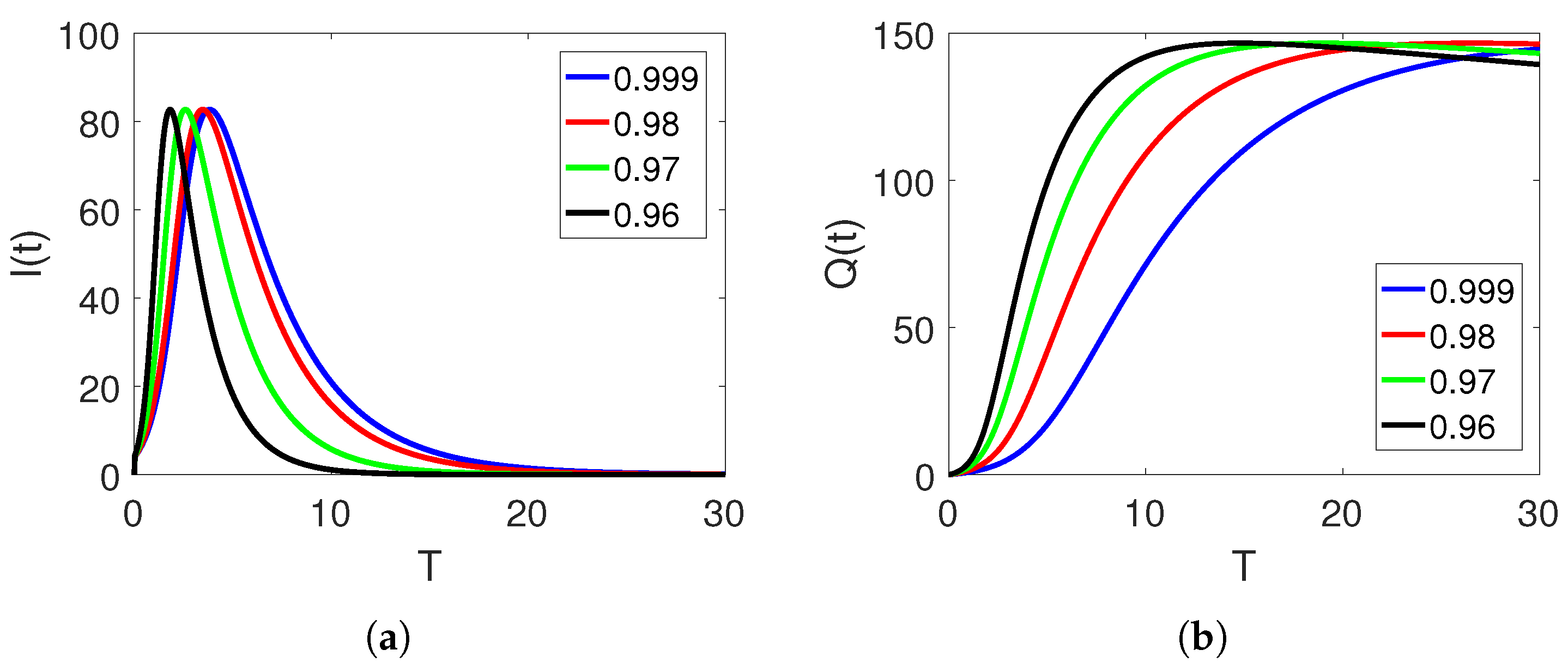
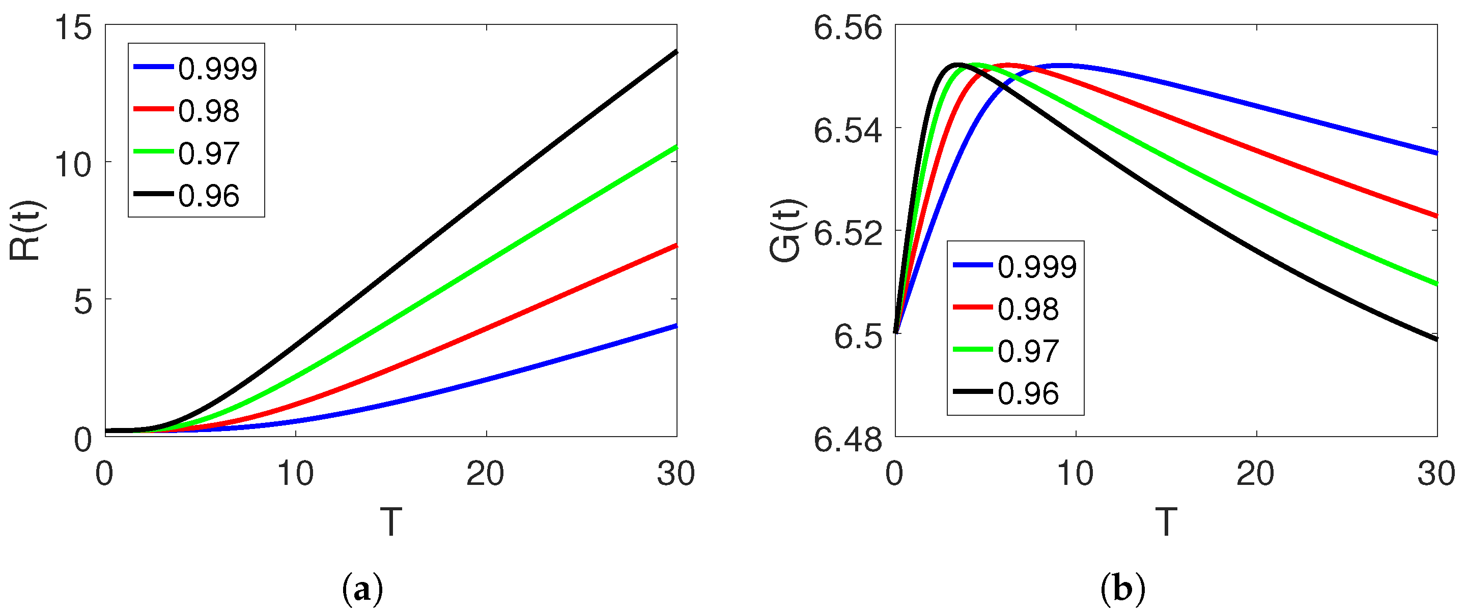
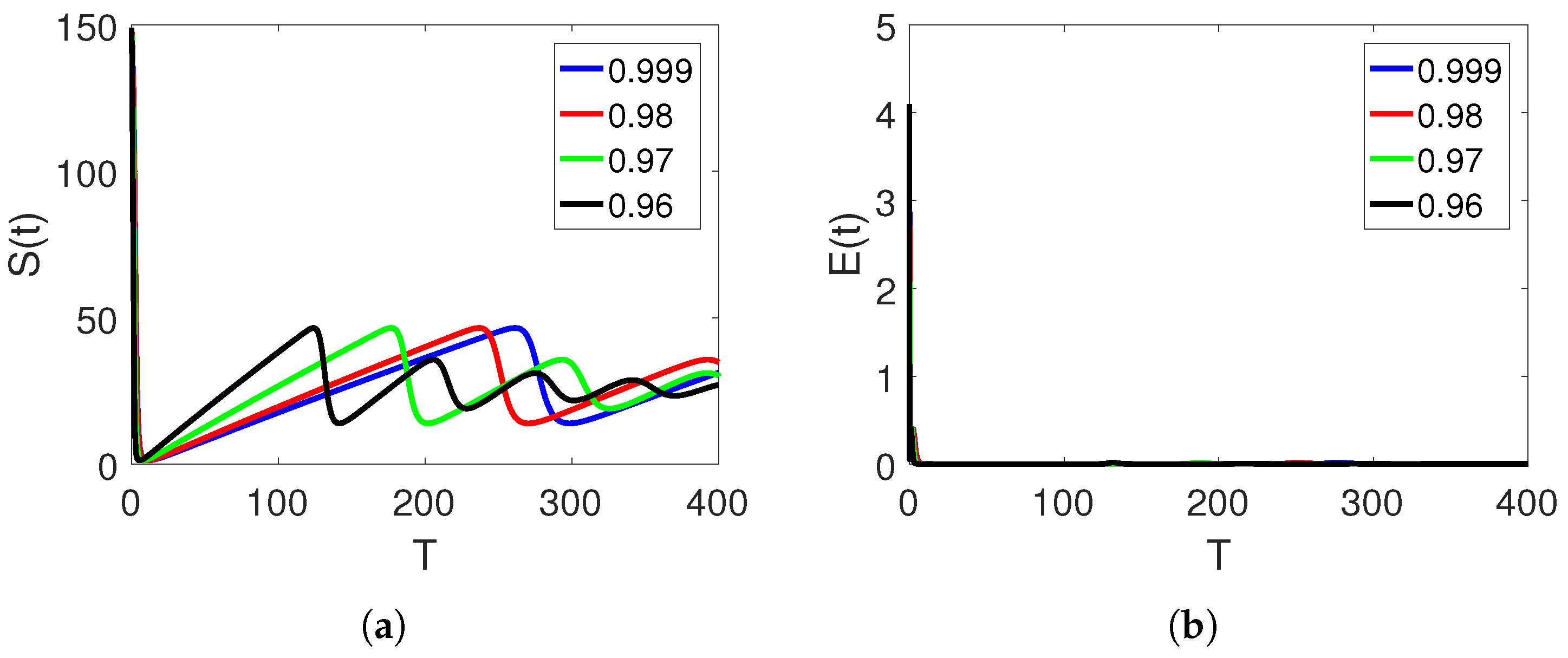
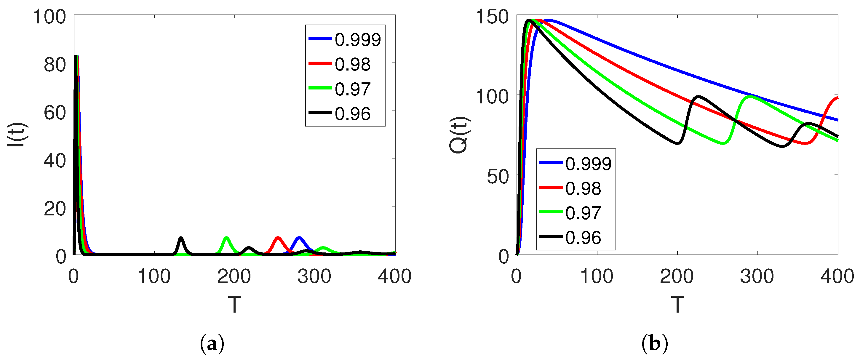
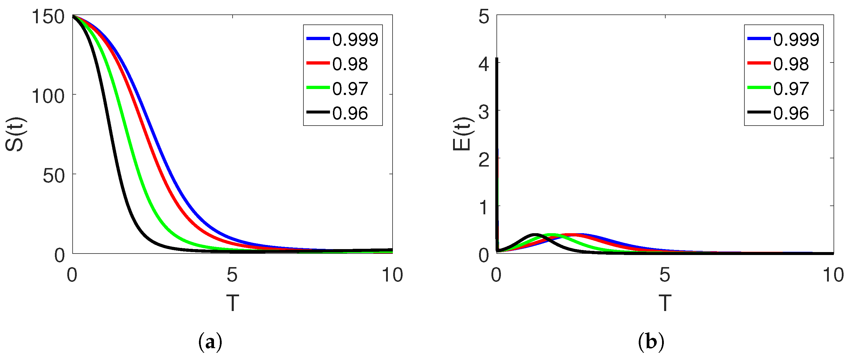
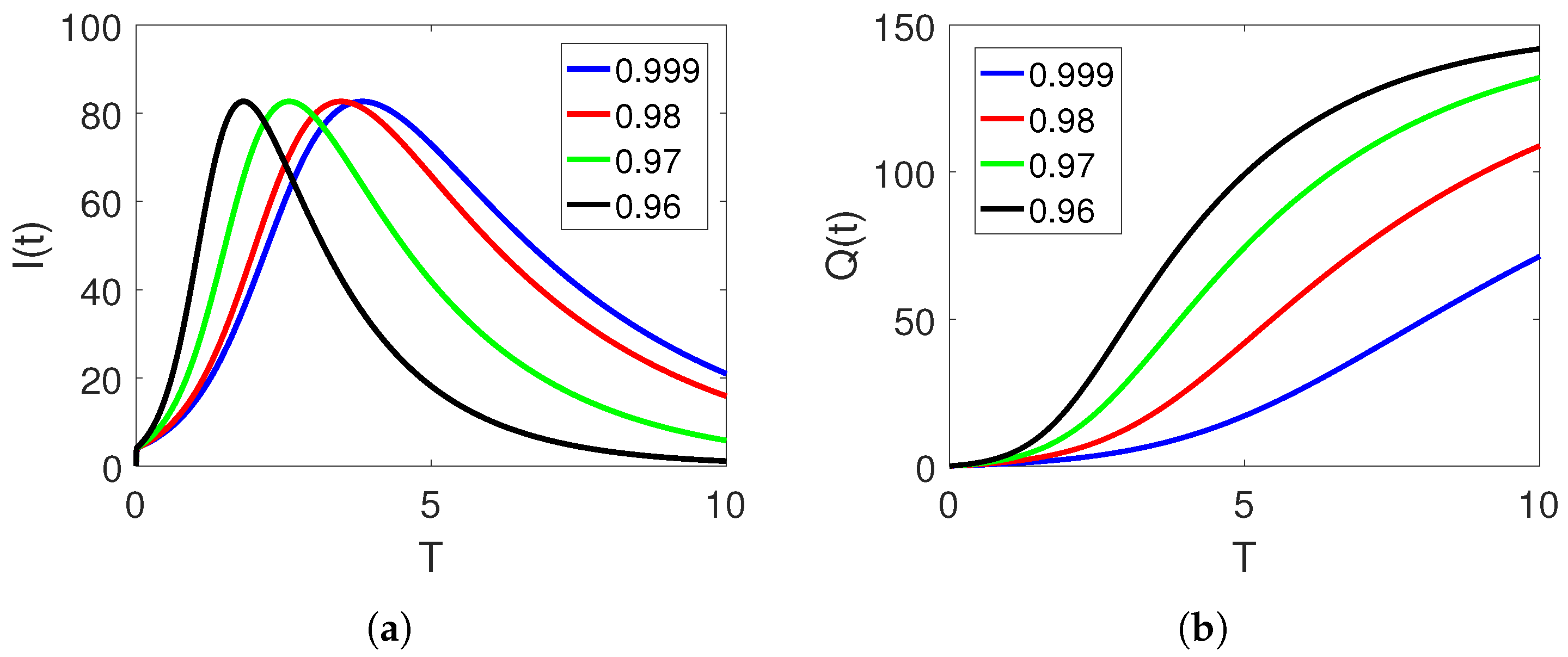
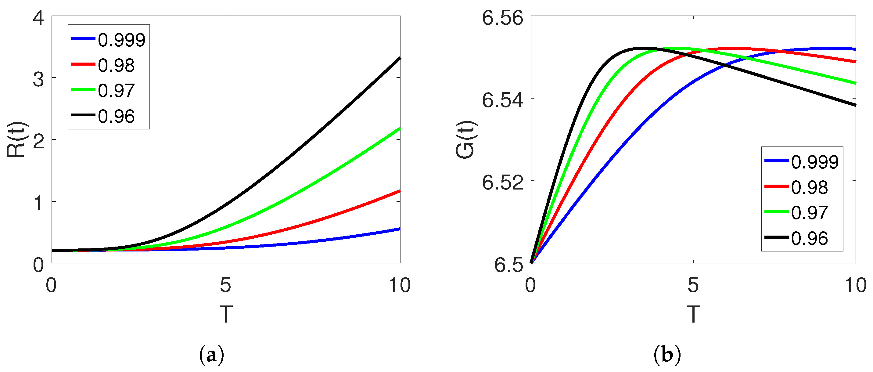
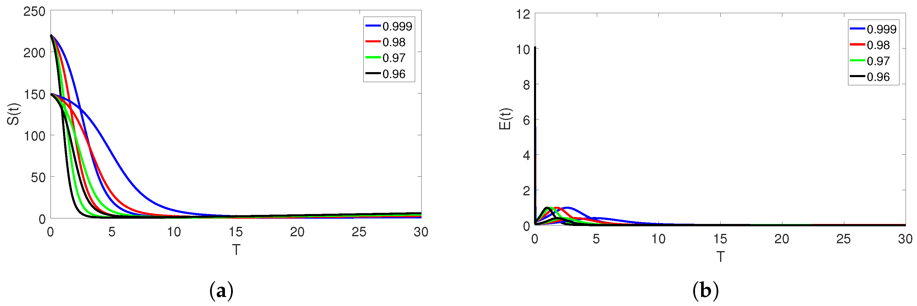
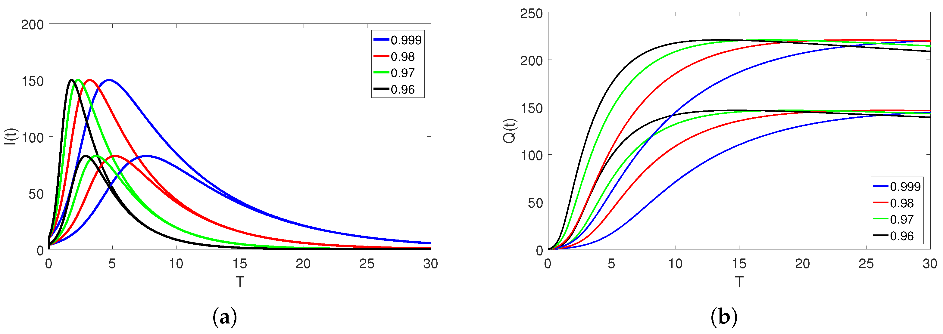
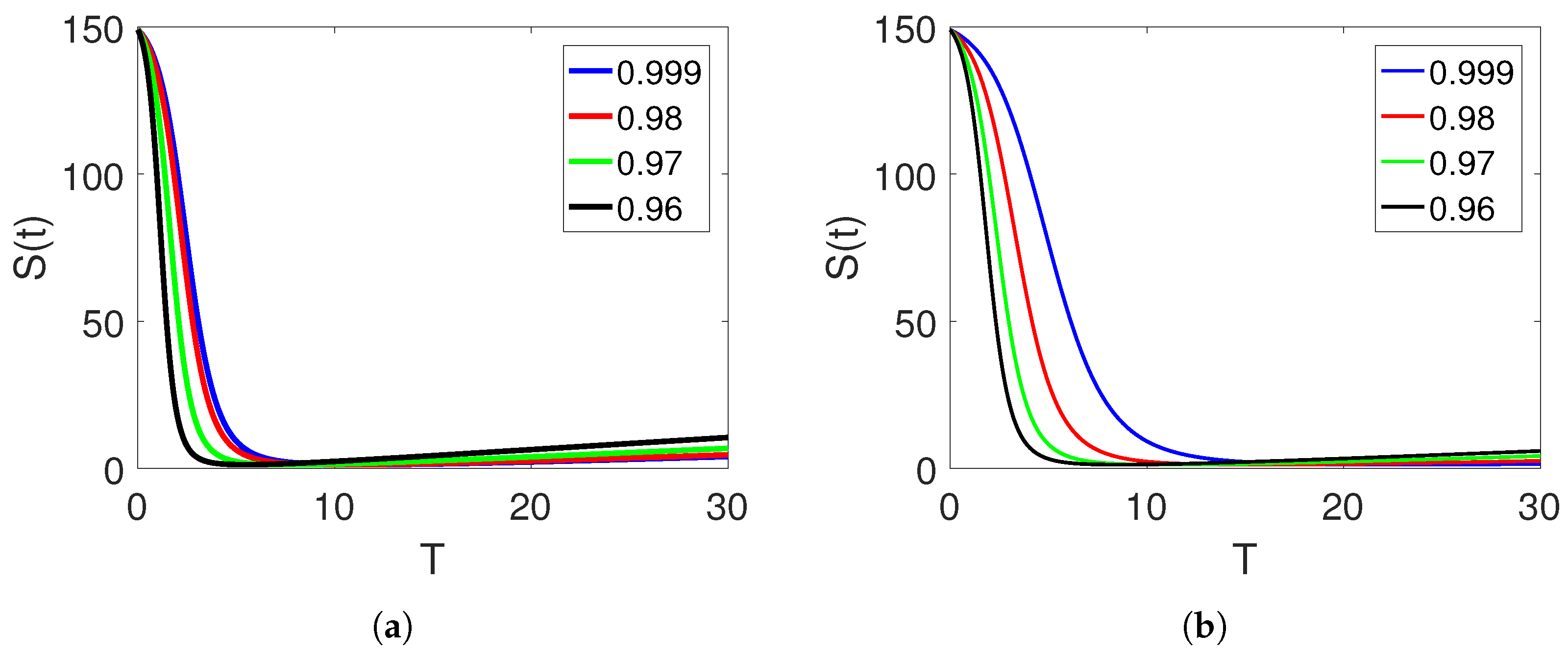
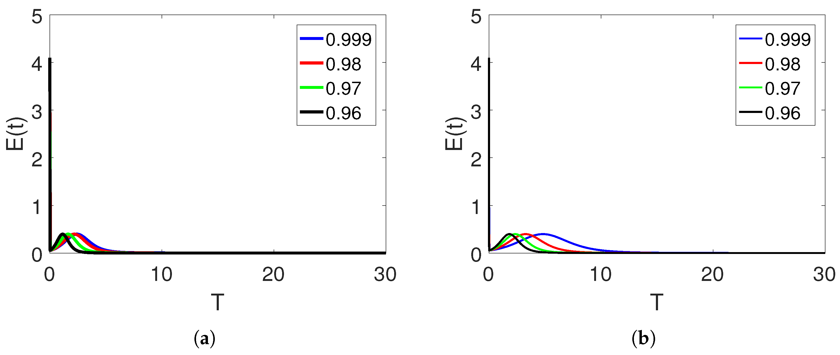
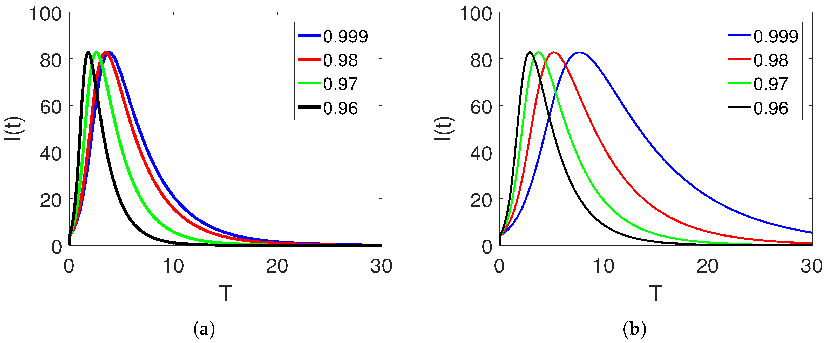
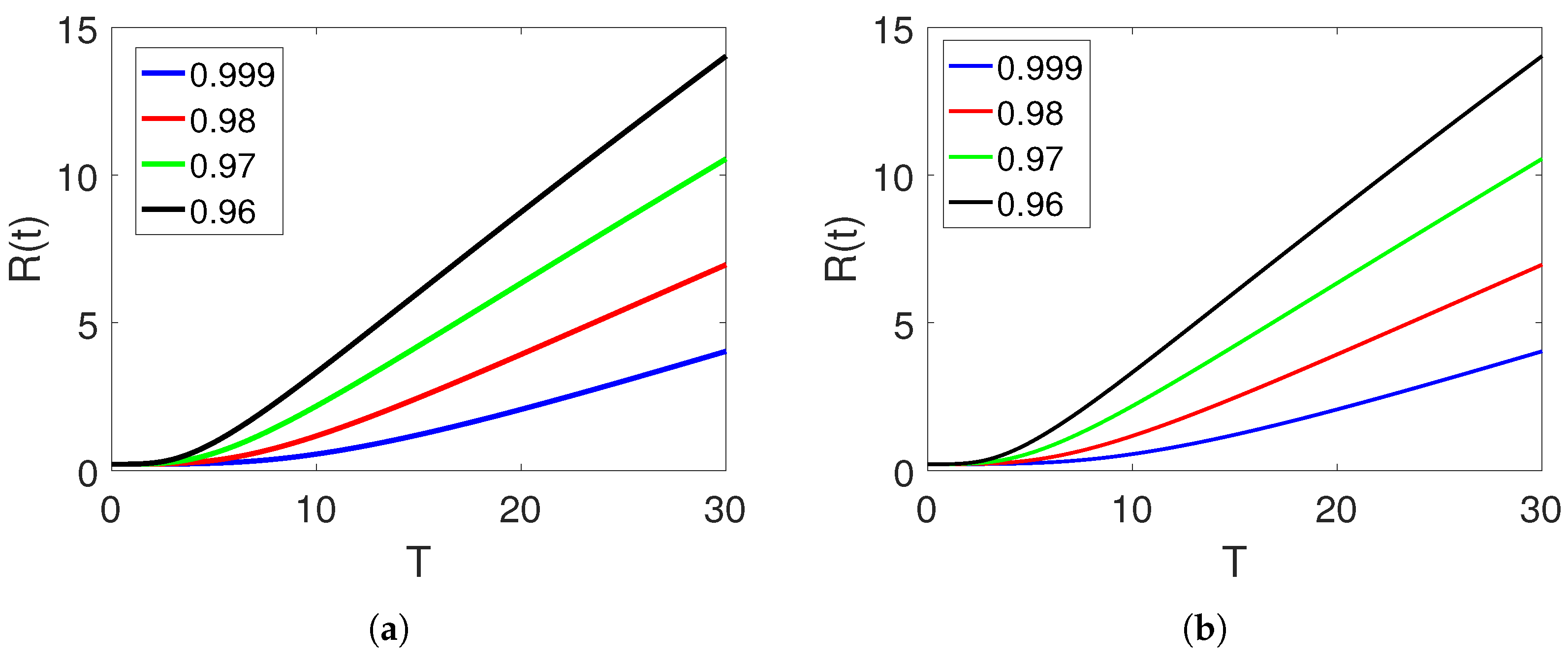
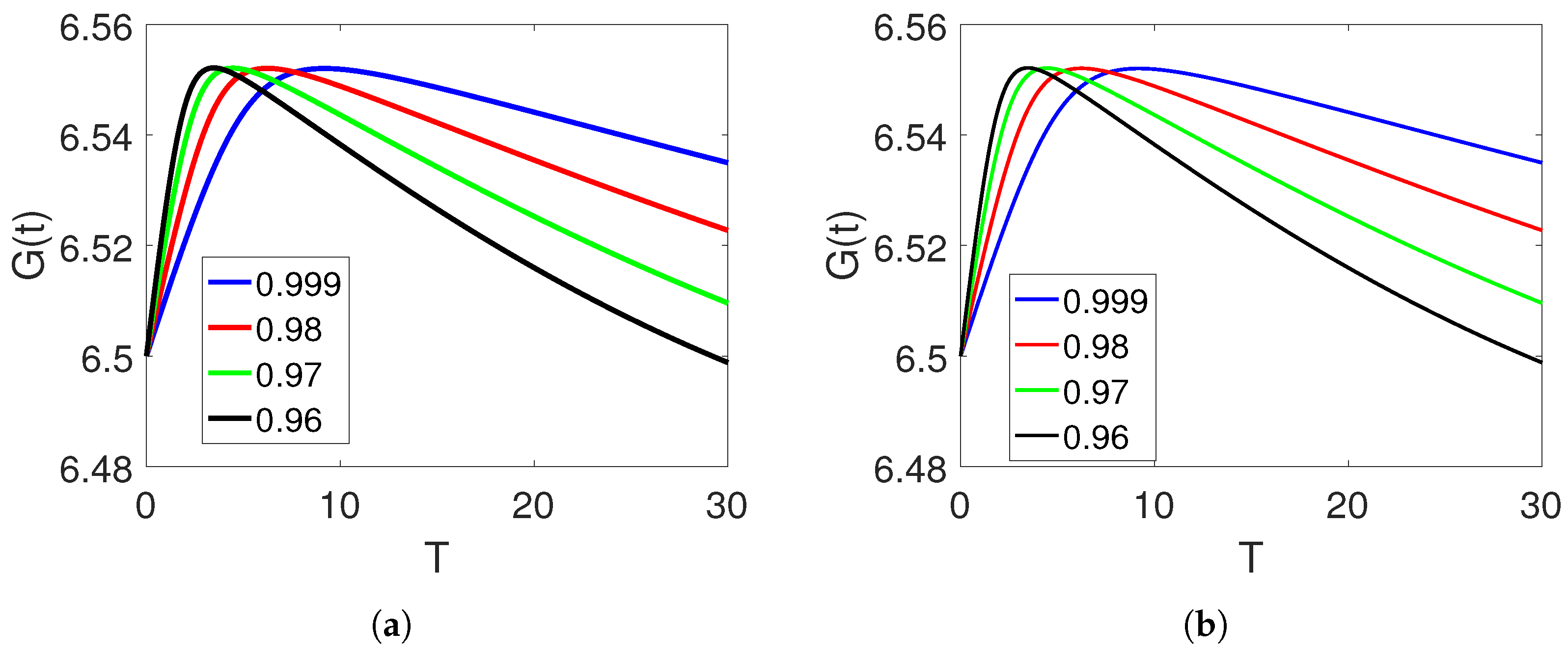
In Figure 1, Figure 2 and Figure 3, we draw the dynamics of all population densities on two subintervals showing bending behavior. We also change the step size in the graphs, showing that the curves are far away from each other in small step sizes and vice versa. The class of susceptible in Figure 1a shows less decay in the first interval while showing more in the second interval, as it transfers to other compartments of the model for all different fractional orders and time duration. The decay is greater at low fractional orders and less at high fractional orders. The exposed population in Figure 1b also declines in both intervals very quickly. The class of infected individuals in Figure 2a gradually increases, reaches the peak value and then declines and becomes stable due to the quarantine and isolation of infected peoples. Figure 2d shows quarantined people who are infected and how their numbers grow and then become stable. Figure 3a,b show the removal and the isolated classes, respectively, which show an increase and then become stable. Figure 4, Figure 5 and Figure 6 show the dynamics with another set of time durations that have the same initial value but change only the final value of time. Figure 7, Figure 8 and Figure 9 are the magnified forms of graphical representation.
All the simulations concluded that assessing the transmission dynamics of the virus based on different values of the parameters depends on the contacts among individuals and elongation in the quarantine period, which are the most effective strategies to combat the pandemic.

Convergence and Comparison

In this subsection, we provide the convergence of all the compartments of the said model in terms of graphical representation with different initial conditions. The graphs are given in Figure 10, Figure 11 and Figure 12. Next, we compare the scheme of Newton interpolation techniques with the Laplace Adomian decomposition method (LADM). A comparison of susceptible individuals is given in Figure 13a,b. Exposed populations are shown in Figure 14a,b. Infected densities are given in Figure 15a,b. Quarantined populations are given in Figure 16a,b. Recovered densities are given Figure 17a,b. Finally, isolated individuals are given in Figure 18a,b.

6. Conclusions

In the investigated model, we developed a novel technique in the sense of a piecewise non-integer-order derivative model of COVID-19 virus infection under Caputo and Atangana–Baleanu fractional operators. The dynamical behavior for the said model was carried out for two subintervals by partitioning the total interval to check the piecewise crossover characteristics. With this manuscript, we will be able to give predictions about the infection dynamics of COVID-19 at two different intervals with changing behaviors. In the first interval, the decrease and increase in all compartments are different from the second one. The qualitative techniques for both the intervals for the considered model solution were developed using the concept of fixed-point theory. The numerical solution was evaluated for the model using Newton’s polynomial procedure for both sub-intervals in Caputo and the ABC framework of order ς . The numerical simulation of all the six compartments was carried out for three different data time durations. The crossover effects were shown by the termination of the first interval, describing the characteristics of the piecewise derivative behaviors. This type of analysis can be applied to real-world dynamical phenomena where an abrupt or sudden variation occurs. This investigation is a more realistic approach, as the dynamics are changing differently at different time durations. Such an analysis describes the crossover properties, which are still not given in deterministic and stochastic problems of both integer and fractional orders.

Author Contributions

Conceptualization and methodology, I.A.; software, validation, and formal analysis, B.S.T.A.; writing—original draft preparation, I.A.; writing—review and editing, B.S.T.A. All authors have read and agreed to the published version of the manuscript.

Funding

This research was supported by the Deanship of Scientific Research, Imam Mohammad Ibn Saud Islamic University (IMSIU), Saudi Arabia, Grant No. (21-13-18-058).

Data Availability Statement

Not applicable.

Conflicts of Interest

The authors declare no conflict of interest.

References

  1. Li, Q.; Guan, X.; Wu, P.; Wang, X.; Zhou, L.; Tong, Y.; Ren, R.; Leung, K.S.; Lau, E.H.; Wong, J.Y.; et al. Early transmission dynamics in Wuhan, China, of novel coronavirus–infected pneumonia. N. Engl. J. Med. 2020, 382, 1199–1207. [Google Scholar] [CrossRef]
  2. Javeed, S.; Ahmed, A.; Khan, M.S.; Javed, M.A. Stability analysis and solutions of dynamical models for Dengue. Punjab Univ. J. Math. 2018, 50, 45–67. [Google Scholar]
  3. Anderson, R.M.; May, R.M. Population biology of infectious diseases: Part I. Nature 1979, 280, 361–367. [Google Scholar] [CrossRef] [PubMed]
  4. Thieme, H.R. Princeton series in theoretical and computational biology. In Mathematics in Population Biology; Princeton University Press: Princeton, NJ, USA, 2003. [Google Scholar]
  5. Luo, X.; Feng, S.; Yang, J.; Peng, X.L.; Cao, X.; Zhang, J.; Yao, M.; Zhu, H.; Li, M.Y.; Wang, H.; et al. Analysis of potential risk of COVID-19 infections in China based on a pairwise epidemic model. Preprints 2020. [Google Scholar] [CrossRef]
  6. Peng, L.; Yang, W.; Zhang, D.; Zhuge, C.; Hong, L. Epidemic analysis of COVID-19 in China by dynamical modeling. arXiv 2020, arXiv:2002.06563. [Google Scholar]
  7. Shao, N.; Zhong, M.; Yan, Y.; Pan, H.S.; Cheng, J.; Chen, W. Dynamic models for Coronavirus Disease 2019 and data analysis. Math. Methods Appl. Sci. 2020, 43, 4943–4949. [Google Scholar] [CrossRef] [PubMed] [Green Version]
  8. Chan, J.F.W.; Yuan, S.; Kok, K.H.; To, K.K.W.; Chu, H.; Yang, J.; Xing, F.; Liu, J.; Yip, C.C.Y.; Poon, R.W.S.; et al. A familial cluster of pneumonia associated with the 2019 novel coronavirus indicating person-to-person transmission: A study of a family cluster. Lancet 2020, 395, 514–523. [Google Scholar] [CrossRef] [Green Version]
  9. Wu, J.T.; Leung, K.; Leung, G.M. Nowcasting and forecasting the potential domestic and international spread of the 2019-nCoV outbreak originating in Wuhan, China: A modelling study. Lancet 2020, 395, 689–697. [Google Scholar] [CrossRef] [Green Version]
  10. Zhao, S.; Lin, Q.; Ran, J.; Musa, S.S.; Yang, G.; Wang, W.; Lou, Y.; Gao, D.; Yang, L.; He, D.; et al. Preliminary estimation of the basic reproduction number of novel coronavirus (2019-nCoV) in China, from 2019 to 2020: A data-driven analysis in the early phase of the outbreak. Int. J. Infect. Dis. 2020, 92, 214–217. [Google Scholar] [CrossRef] [Green Version]
  11. Tang, B.; Bragazzi, N.L.; Li, Q.; Tang, S.; Xiao, Y.; Wu, J. An updated estimation of the risk of transmission of the novel coronavirus (2019-nCov). Infect. Dis. Model. 2020, 5, 248–255. [Google Scholar] [CrossRef]
  12. Batista, M. Estimation of the final size of the COVID-19 epidemic. MedRxiv 2020. [Google Scholar] [CrossRef] [Green Version]
  13. Kermack, W.O.; McKendrick, A.G. A contribution to the mathematical theory of epidemics. Proc. R. Soc. Lond. Ser. A Contain. Pap. Math. Phys. Character 1927, 115, 700–721. [Google Scholar]
  14. Anderson, R.M.; May, R.M. Directly transmitted infections diseases: Control by vaccination. Science 1982, 215, 1053–1060. [Google Scholar] [CrossRef] [PubMed]
  15. Dietz, K. The incidence of infectious diseases under the influence of seasonal fluctuations. In Mathematical Models in Medicine; Springer: Berlin/Heidelberg, Germany, 1976; pp. 1–15. [Google Scholar]
  16. Tang, B.; Wang, X.; Li, Q.; Bragazzi, N.L.; Tang, S.; Xiao, Y.; Wu, J. Estimation of the transmission risk of the 2019-nCoV and its implication for public health interventions. J. Clin. Med. 2020, 9, 462. [Google Scholar] [CrossRef] [Green Version]
  17. Khan, M.A.; Atangana, A.; Alzahrani, E. The dynamics of COVID-19 with quarantined and isolation. Adv. Differ. Equ. 2020, 2020, 1–22. [Google Scholar] [CrossRef]
  18. Memon, Z.; Qureshi, S.; Memon, B.R. Memon, Assessing the role of quarantine and isolation as control strategies for COVID-19 outbreak: A case study. Chaos Solitons Fractals 2021, 144, 110655. [Google Scholar] [CrossRef] [PubMed]
  19. Javeed, S.; Anjum, S.; Alimgeer, K.S.; Atif, M.; Khan, M.S.; Farooq, W.A.; Hanif, A.; Ahmad, H.; Yao, S.W. A novel mathematical model for COVID-19 with remedial strategies. Results Phys. 2021, 27, 104248. [Google Scholar] [CrossRef]
  20. Atangana, A.; Baleanu, D. New fractional derivatives with non-local and non-singular kernel. Theory Appl. Heat Transf. Model Therm. Sci. 2016, 20, 763–769. [Google Scholar]
  21. Goufo, E.F.D. Application of the Caputo-Fabrizio fractional derivative without singular kernel to Korteweg-de Vries-Burgers equation. Math. Model. Anal. 2016, 21, 188–198. [Google Scholar] [CrossRef]
  22. Goufo, E.F.D. A bio mathematical view on the fractional dynamics of cellulose degradation. Fract. Calc. Appl. Anal. 2015, 18, 554–564. [Google Scholar] [CrossRef]
  23. Atangana, A. Extension of rate ofchange concept:from local to nonlocal operators with applications. Results Phys. 2020, 19, 103515. [Google Scholar] [CrossRef]
  24. Atangana, A.; Araz, S.I. Nonlinear equations with global differential and integral operators: Existence, uniqueness with application to epidemiology. Results Phys. 2020, 20, 103593. [Google Scholar] [CrossRef]
  25. Kabunga, S.K.; Goufo, E.F.D.; Tuong, V.H. Analysis and simulation of a mathematical model of tuberculosis transmission in democratic Republic of the Congo. Adv. Differ. Equ. 2020, 2020, 642. [Google Scholar] [CrossRef]
  26. Atangana, A.; Araz, S.I. Mathematical model of COVID-19 spread in Turkey and South Africa: Theory, methods and applications. Adv. Differ. Equ. 2020, 2020, 659. [Google Scholar] [CrossRef]
  27. Atangana, A.; Araz, S.I. New concept in calculus: Piecewise differential and integral operators. Chaos Solitons Fractals 2021, 145, 110638. [Google Scholar] [CrossRef]
  28. Arfan, M.; Shah, K.; Ullah, A.; Salahshour, S.; Ahmadian, A.; Ferrara, M. A novel semi-analytical method for solutions of two dimensional fuzzy fractional wave equation using natural transform. Discret. Contin. Dyn. Syst. 2022, 15, 315–338. [Google Scholar] [CrossRef]
  29. ur Rahman, M.; Arfan, M.; Shah, Z.; Kumam, P.; Shutaywi, M. Nonlinear fractional mathematical model of tuberculosis (TB) disease with incomplete treatment under Atangana-Baleanu derivative. Alex. Eng. J. 2021, 60, 2845–2856. [Google Scholar] [CrossRef]
  30. Arfan, M.; Alrabaiah, H.; Rahman, M.U.; Sun, Y.L.; Hashim, A.S.; Pansera, B.A.; Ahmadian, A.; Salahshour, S. Investigation of fractal-fractional order model of COVID-19 in Pakistan under Atangana-Baleanu Caputo (ABC) derivative. Results Phys. 2021, 24, 104046. [Google Scholar] [CrossRef]
  31. Podlubny, I. Geometric and physical interpretation of fractional integration and fractional differentiation. Fract. Calc. Appl. Anal. 2002, 5, 367–386. [Google Scholar]
  32. Verhulst, P.F. Notice sur la loi que la population suit dans son accroissement. Corresp. Math. Phys. 1838, 10, 113–121. (In French) [Google Scholar]
  33. Fabiano, N.; Radenovic, S. Geometric Brownian motion and a new approach to the spread of covid-19 in Italy. Gulf J. Math. 2021, 10, 25–30. [Google Scholar] [CrossRef]
  34. Fabiano, N.; Radenovic, S. On COVID-19 diffusion in italy: Data analysis and possible Vojnotehni? Vojnoteh. Glas./Mil. Tech. Cour. 2020, 68, 216–224. [Google Scholar] [CrossRef]
  35. Debnath, P.; Konwar, N.; Radenovic, S. Metric Fixed Point Theory, Applications in Sciences, Engineering and Behavioural Sciences; Springer: Berlin/Heidelberg, Germany, 2021. [Google Scholar]
  36. Baleanu, D.; Arshad, S.; Jajarmi, A.; Shokat, W.; Ghassabzade, F.A.; Wali, M. Dynamical behaviours and stability analysis of a generalized fractional model with a real case study. J. Adv. Res. 2022; in press. [Google Scholar]
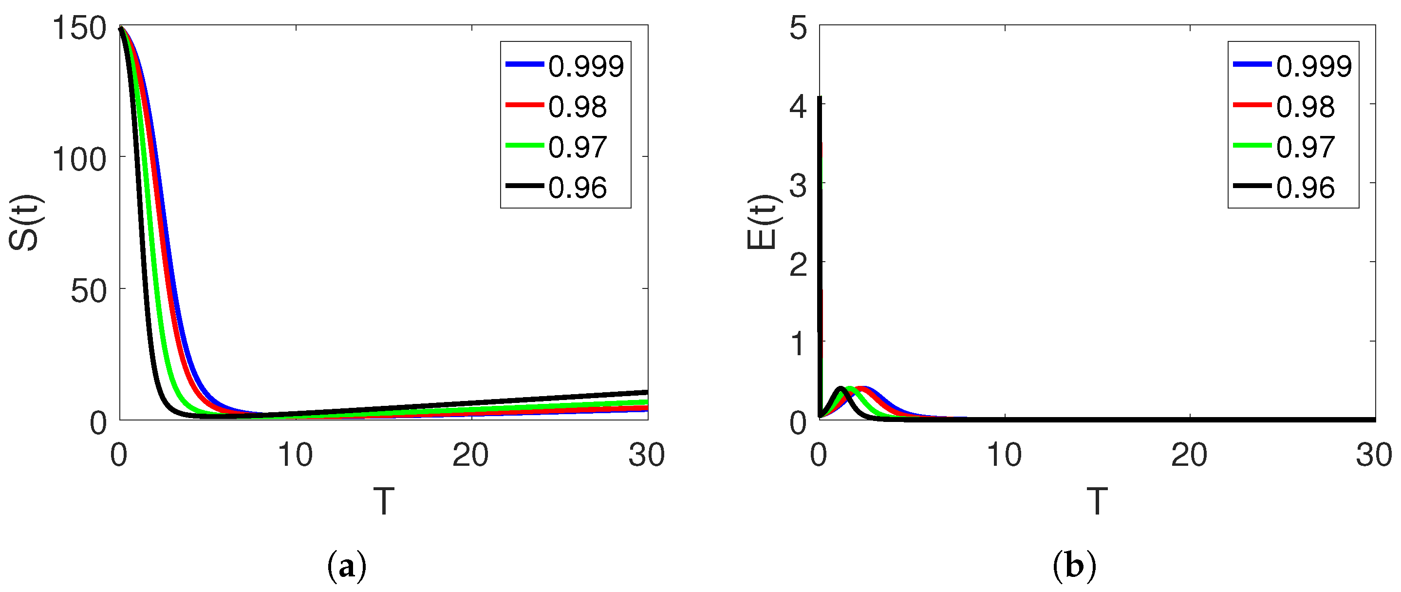
Figure 1. Dynamics of the susceptible class (a) and exposed class (b) on different arbitrary fractional order ς on sub interval [ 0 , t 1 ] and [ t 1 , T ] of [ 0 , T ] .
Fractalfract 06 00661 g001
Figure 2. Dynamics of the infected class (a) and quarantined class (b) on different arbitrary fractional order ς on sub interval [ 0 , t 1 ] and [ t 1 , T ] of [ 0 , T ] .
Fractalfract 06 00661 g002
Figure 3. Dynamical behavior of the recovered class (a) and isolated class (b) on different arbitrary fractional order ς on sub interval [ 0 , t 1 ] and [ t 1 , T ] of [ 0 , T ] .
Fractalfract 06 00661 g003
Figure 4. Dynamics of the susceptible class (a) and exposed class (b) on different arbitrary fractional order ς on sub interval [ 0 , t 1 ] and [ t 1 , T ] of [ 0 , T ] for different time duration.
Fractalfract 06 00661 g004
Figure 5. Dynamics of the infected class (a) and quarantined class (b) on different arbitrary fractional order ς on sub interval [ 0 , t 1 ] and [ t 1 , T ] of [ 0 , T ] for different time duration.
Fractalfract 06 00661 g005
Figure 6. Dynamical behavior of the recovered class (a) and isolated class (b) on different arbitrary fractional order ς on sub interval [ 0 , t 1 ] and [ t 1 , T ] of [ 0 , T ] for different time duration.
Fractalfract 06 00661 g006
Figure 7. Dynamics of the susceptible class (a) and exposed class (b) on different arbitrary fractional order ς on sub interval [ 0 , t 1 ] and [ t 1 , T ] of [ 0 , T ] for different time duration.
Fractalfract 06 00661 g007
Figure 8. Dynamics of the infected class (a) and quarantined class (b) on different arbitrary fractional order ς on sub interval [ 0 , t 1 ] and [ t 1 , T ] of [ 0 , T ] for different time duration.
Fractalfract 06 00661 g008
Figure 9. Dynamical of the recovered class (a) and isolated class (b) on different arbitrary fractional order ς on sub interval [ 0 , t 1 ] and [ t 1 , T ] of [ 0 , T ] for different time duration.
Fractalfract 06 00661 g009
Figure 10. Dynamical behavior of the susceptible class (a) and exposed class (b) on different arbitrary fractional order ς on sub interval [ 0 , t 1 ] and [ t 1 , T ] of [ 0 , T ] , for different initial values.
Fractalfract 06 00661 g010
Figure 11. Dynamical behavior of the infected class (a) and quarantined class (b) on different arbitrary fractional order ς on sub interval [ 0 , t 1 ] and [ t 1 , T ] of [ 0 , T ] , for different initial values.
Fractalfract 06 00661 g011
Figure 12. Dynamical behavior of the recovered class (a) and isolated class (b) on different arbitrary fractional order ς on sub interval [ 0 , t 1 ] and [ t 1 , T ] of [ 0 , T ] , for different initial values.
Fractalfract 06 00661 g012
Figure 13. Comparison of Newton polynomial (a) and LADM (b) for first class on different arbitrary fractional order.
Fractalfract 06 00661 g013
Figure 14. Comparison of Newton polynomial (a) and LADM (b) for second class on different arbitrary fractional order.
Fractalfract 06 00661 g014
Figure 15. Comparison of Newton polynomial (a) and LADM (b) for third class on different arbitrary fractional order.
Fractalfract 06 00661 g015
Figure 16. Comparison of Newton polynomial (a) and LADM (b) for fourth class on different arbitrary fractional order.
Fractalfract 06 00661 g016
Figure 17. Comparison of Newton polynomial (a) and LADM (b) for fifth class on different arbitrary fractional order.
Fractalfract 06 00661 g017
Figure 18. Comparison of Newton polynomial (a) and LADM (b) for sixth class on different arbitrary fractional order.
Fractalfract 06 00661 g018
Table 1. Description of the parameter of (1).
NotationDetails
Λ 27.530/1000
α E 0.004253392
α I 3.245065087
δ 0.003505
μ 6.884/1000
β 0.0003551
γ 0.1597073
r0.058306850
d0.00414502
Publisher’s Note: MDPI stays neutral with regard to jurisdictional claims in published maps and institutional affiliations.