Fractional View Analysis of Swift–Hohenberg Equations by an Analytical Method and Some Physical Applications

Abstract

This study investigates the fractional-order Swift–Hohenberg equations using the natural decomposition method with non-singular kernel derivatives. The fractional derivative in the sense of Caputo–Fabrizio is considered. The Adomian decomposition technique (ADT) is a great deal to the overall natural transformation to create closed-form results of the given models. This technique provides a closed-form result for the suggested models. In addition, this technique is attractive, simple, and preferred over other techniques. The graphs of the solution in fractional and integer-order show that the achieved solutions are very close to the actual result of the examples. It is also investigated that the result of fractional-order models converges to the integer-order model’s solution. Furthermore, the proposed method validity is examined using numerical examples. The obtained results for the given problems fully support the theory of the proposed method. The present method is a straightforward and accurate analytical method to analyze other fractional-order partial differential equations, such as many evolution equations that govern the dynamics of nonlinear waves in plasma physics.

1. Introduction

Fractional calculus (FC) has become an essential computational method for describing appropriate nonlocal problems. Fractional derivatives have mathematically interpreted many physical models in the last few centuries; these representations have generated outstanding solutions to real-world modeling problems. Riemann–Liouville, Coimbra, Weyl, Riesz, Liouville–Caputo, Hadamard, Grunwald–Letnikov, Caputo–Fabrizio, Atangana–Baleanu, and others, provided numerous fundamental ideas for the fractional operators [1,2]. The Caputo–Fabrizio fractional derivative has expanded our understanding of fractional differential equations. The new derivative’s charm is that it has a non-singular kernel. The Caputo–Fabrizio derivative combines an ordinary derivative and an exponential function. Still, it has the same additional driving qualities of heterogeneity and configuration with different scales as the Caputo and Riemann–Liouville fractional derivatives. Over the last several years, various nonlinear problems have been established and broadly utilized in nonlinear scientific fields such as mathematics, biological sciences, chemistry, and other aspects of mechanics such as thermodynamics, condensed matter physics, quantum dynamics, wave equation, optics, and plasma physics. The accurate result of nonlinear systems is essential in deciding the characteristics and properties of physical processes. Still, sometimes it is difficult to obtain accurate results when dealing with nonlinear problems [3,4,5,6]. Since the field of partial differential equations (PDEs) is so significant in modeling several real-world issues, nonlinear equations are also fundamental in developing different models and problems in materials science, fluid dynamics, communications, plasma physics, and industrial engineering. As a result, these equations have been examined analytically and numerically using different techniques [7,8,9]. The equations above have been examined under numerous fractional differential operators [3,10,11,12] due to the applications of fractional calculus. Keeping in mind the significance of PDEs, the ”Swift–Hohenberg equation” is a significant problem that precisely represents the evolution and generation of patterns in many systems. Swift and Hohenberg are the first to develop the Swift–Hohenberg equation: [13]

$$\frac{\partial \rho }{\partial \overline{\Im }}=\eta \overline{\zeta }-{\left(1+{\nabla }^2\right)}^2\rho +N\left(\rho \right).$$

Here, $N\left(\overline{\zeta }\right)$ is a nonlinear term, $\eta$ is a real constant, and $\rho$ is a scalar function. A fundamental partial differential equation that defines pattern creation in various physical systems is the Swift–Hohenberg equation. J. discovered this equation for the first time. P. Swift and Hohenberg has the form and is useful for characterizing the hydrodynamic fluctuations near the convective instability.

$${\rho }_{\overline{\Im }}+2{\rho }_{\overline{\zeta }\overline{\zeta }}+{\rho }_{\overline{\zeta }\overline{\zeta }\overline{\zeta }\overline{\zeta }}=\alpha \rho +\beta {\rho }^2-\gamma {\rho }^3,$$

(1)

where $\alpha ,\beta$ and $\gamma$ are constant parameters of equation. This equation appears in numerous scientific disciplines. It explains, for instance, how shear microbands in nanocrystalline materials arise, the size of the optical electric field inside a cavity, the patterns found inside thin vibrated granular layers, and many other things. Studying the wave mechanisms that this equation and its generalizations explain is crucial. One of the interesting generalizations of Equation (1), arises in literature, have the following form

$${\rho }_{\overline{\Im }}+2{\rho }_{\overline{\zeta }\overline{\zeta }}-\sigma {\rho }_{\overline{\zeta }\overline{\zeta }\overline{\zeta }}+{\rho }_{\overline{\zeta }\overline{\zeta }\overline{\zeta }\overline{\zeta }}=\alpha \rho -\gamma {\rho }^{m+1},$$

(2)

where $\sigma ,\alpha$ and $\gamma$ are the parameters. In Ref. [5], authors define the existence condition of non stationary meromorphic solutions of Equation (2), that corresponds to $\sigma \ne 0$. Using this fact they were succeed to find elliptic and simple periodic solutions. Another work, devoted to studding the Equation (2) is a work, where the so-called snakes-and-ladders structure of equation is studied. The Swift–Hohenberg equation has various uses in engineering and science, including physics, biology, fluid, laser research and hydro dynamics [14,15,16]. In addition, this equation has various uses in pattern formation modeling and its numerous difficulties, such as the impact of noise on bifurcations, pattern selection, defect dynamics, and spatiotemporal chaos [17,18,19,20]. The Swift–Hohenberg equation [21] is crucial in pattern creation theory in fluid layers restricted between horizontal well-conducting barriers.

In the present investigation, we consider the fractional Swift–Hohenberg equations with three different forms; for the initial two forms, [22,23,24].

Type-I

Swift–Hohenberg equations:

$$\begin{array}{cc}& {}^{CF}{D}_{\overline{\Im }}^{\beta }\rho (\overline{\zeta },\overline{\Im })+\frac{{\partial }^4\left(\rho (\overline{\zeta },\overline{\Im })\right)}{\partial {\overline{\zeta }}^4}+2\frac{{\partial }^2\left(\rho (\overline{\zeta },\overline{\Im })\right)}{\partial {\overline{\zeta }}^2}+(1-\vartheta )\rho (\overline{\zeta },\overline{\Im })+{\rho }^3(\overline{\zeta },\overline{\Im })=0,\beta \in (0,1],\vartheta \in R,\overline{\Im }>0,\hfill \end{array}$$

Type-II

Swift–Hohenberg equations:

$$\begin{array}{cc}& {}^{CF}{D}_{\overline{\Im }}^{\beta }\rho (\overline{\zeta },\overline{\Im })+\frac{{\partial }^4\left(\rho (\overline{\zeta },\overline{\Im })\right)}{\partial {\overline{\zeta }}^4}+2\frac{{\partial }^2\left(\rho (\overline{\zeta },\overline{\Im })\right)}{\partial {\overline{\zeta }}^2}+(1-\vartheta )\rho (\overline{\zeta },\overline{\Im })={\rho }^{\ell }(\overline{\zeta },\overline{\Im })-{\left(\frac{\partial \rho (\overline{\zeta },\overline{\Im })}{\partial \overline{\zeta }}\right)}^{\ell },\beta \in (0,1],\overline{\Im }>0,\hfill \end{array}$$

where $\vartheta \in R$ and $\ell \ge 0$.

Type-III

Swift–Hohenberg equations:

In the presence of the dispersive function [25], we investigate the proposed model of the Swift–Hohenberg equation:

$$\begin{array}{cc}& {}^{CF}{D}_{\overline{\Im }}^{\beta }\rho (\overline{\zeta },\overline{\Im })+\frac{{\partial }^4\left(\rho (\overline{\zeta },\overline{\Im })\right)}{\partial {\overline{\zeta }}^4}+2\frac{{\partial }^2\left(\rho (\overline{\zeta },\overline{\Im })\right)}{\partial {\overline{\zeta }}^2}-\kappa \frac{{\partial }^3\left(\rho (\overline{\zeta },\overline{\Im })\right)}{\partial {\overline{\zeta }}^3}-\lambda \rho (\overline{\zeta },\overline{\Im })-2{\rho }^2(\overline{\zeta },\overline{\Im })+{\rho }^3(\overline{\zeta },\overline{\Im })=0,\hfill \end{array}$$

where ${}^{CF}{D}_{\overline{\Im }}^{\beta }$ is Caputo–Fabrizio fractional operator and $\lambda ,\kappa$ are bifurcation and dispersive real parameters. Many researchers analyzed and solved the Swift–Hohenberg equation using various methodologies, such as Vishal et al.’s use of the homotopy analysis method [22] and the homotopy perturbation transform method. Moreover, the Swift–Hohenberg equation was solved using the variational iteration method with the Riemann–Liouville derivative and the differential transform method. Motivated by the preceding work, we establish an approximation analytic solution for the given problem using a computer known as the natural decomposition method (NDM). We also present a convergence analysis for the problem under consideration. To fulfill this requirement, Maitama and Rawashdeh introduced and nurtured the fractional NDM [26,27], a mixture of the ADT and the natural transform method. Since the fractional NDM is an improved method of ADT, it will reduce vast computations, and in addition, it does not requires discretization, linearization, or perturbation. Recently, due to the efficacy and reliability of the projected scheme; thus, several researchers worked on it to understand the mystery of various nonlinear models [28,29,30].

Due to the future technique allows us to choose the equation type of linear subproblems, the initial guess, and the base function of the solution; thus, sophisticated nonlinear differential equations can often be solved. The proposed technique is unique in that it has a broad convergence zone, a straightforward solution procedure, and a nonlocal effect in the achieved solution. The future scheme manages and manipulates the series solution, which swiftly converges to the exact answer in a narrow acceptable region, which no other traditional techniques can achieve. Furthermore, it logically contains the results of some traditional methods, such as the ADT, the homotopy perturbation method (HPM), the q-homotopy analysis transform method, and the reduced differential transforms method, giving it prodigious generality. It is worth noting that the proposed approach can reduce computing time and work compared to other standard procedures while retaining highly efficient results obtained.

2. Basic Definitions

Definition 1.

The Riemann–Liouville fractional integral operator of a function $f\in C_v,v\ge -1$ is defined as [31]

$$\begin{array}{cc}\hfill I^{\beta }f\left(\omega \right)=& \frac{1}{\Gamma \left(\beta \right)}{\int }_0^{\omega }{(\omega -\zeta )}^{\beta -1}f\left(\zeta \right)d\zeta ,\beta >0,\omega >0.\hfill \\ \hfill and{I}^{0}f\left(\omega \right)=& f\left(\omega \right).\hfill \end{array}$$

(3)

Definition 2.

The fractional Caputo operator of $f\left(\omega \right)$ is given as [31]

$$\begin{array}{c}\hfill D_{\omega }^{\beta }f\left(\omega \right)=I^{\ell -\beta }{D}^{\ell }f\left(\omega \right)=\frac{1}{\ell -\beta }{\int }_{\omega }^0{(\omega -\zeta )}^{\ell -\beta -1}{f}^{\ell }\left(\zeta \right)d\zeta ,\end{array}$$

(4)

for $\ell -1<\beta \le \ell ,\ell \in N,\omega >0,f\in C_v^{\ell },v\ge -1$.

Definition 3.

The fractional Caputo–Fabrizio derivative of $f\left(\omega \right)$ is given as [31]

$$\begin{array}{c}\hfill D_{\omega }^{\beta }f\left(\omega \right)=\frac{B\left(\beta \right)}{1-\beta }{\int }_0^{\omega }exp\left(\frac{-\beta (\omega -\zeta )}{1-\beta }\right)D\left(f\left(\zeta \right)\right)d\zeta ,\end{array}$$

(5)

where $0<\beta <1$ and $B\left(\beta \right)$ is a normalization function, where $B\left(0\right)=B\left(1\right)=1$.

Definition 4.

The Natural transform of $\phi \left(\overline{\Im }\right)$ is defined by [31]

$$\begin{array}{c}\hfill \mathcal{N}\left(\phi \left(\overline{\Im }\right)\right)=\mathcal{U}(s,v)={\int }_{-\infty }^{\infty }{e}^{-s\overline{\Im }}\phi (v,\overline{\Im })d\overline{\Im },s,v\in (-\infty ,\infty ).\end{array}$$

(6)

For $\overline{\Im }\in (0,\infty )$, Natural transformation of $\phi \left(\overline{\Im }\right)$ is given by

$$\begin{array}{c}\hfill \mathcal{N}\left(\phi \left(\overline{\Im }\right)H\left(\overline{\Im }\right)\right)={\mathcal{N}}^{+}={\mathcal{U}}^{+}(s,v)={\int }_0^{\infty }{e}^{-s\overline{\Im }}\phi (v,\overline{\Im })d\overline{\Im },s,v\in (0,\infty ).\end{array}$$

(7)

where $H\left(\overline{\Im }\right)$ is the Heaviside term.

Definition 5.

The inverse Natural transform of $\mathcal{U}(s,v)$ is define as [31]

$$\begin{array}{c}\hfill {\mathcal{N}}^{-1}\left[\mathcal{U}(s,v)\right]=\phi \left(\overline{\Im }\right),\forall \overline{\Im }\ge 0.\end{array}$$

(8)

Lemma 1.

If linearity property of Natural transform of ${\phi }_1\left(\overline{\Im }\right)$ is ${\phi }_1(s,v)$ and ${\phi }_2\left(\overline{\Im }\right)$ is ${\phi }_2(s,v)$, then [31]

$$\begin{array}{c}\hfill \mathcal{N}[c_1{\phi }_1\left(\overline{\Im }\right)+c_2{\phi }_2\left(\overline{\Im }\right)]=c_1\mathcal{N}\left[{\phi }_1\left(\overline{\Im }\right)\right]+c_2\mathcal{N}\left[{\phi }_2\left(\overline{\Im }\right)\right]=c_1{\phi }_1(s,v)+c_2{\phi }_2(s,v),\end{array}$$

(9)

where $c_1$ and $c_2$ are constants.

Lemma 2.

If inverse Natural transformation of ${\phi }_1(s,v)$ and ${\phi }_2(s,v)$ are ${\phi }_1\left(\overline{\Im }\right)$ and ${\phi }_2\left(\overline{\Im }\right)$ respectively [31] then

$$\begin{array}{c}\hfill {\mathcal{N}}^{-1}[c_1{\phi }_1(s,v)+c_2{\phi }_2(s,v)]=c_1{\mathcal{N}}^{-1}\left[{\phi }_1(s,v)\right]+c_2{\mathcal{N}}^{-1}\left[{\phi }_2(s,v)\right]=c_1{\phi }_1\left(\overline{\Im }\right)+c_2{\phi }_2\left(\overline{\Im }\right),\end{array}$$

(10)

where $c_1$ and $c_2$ are constants.

Definition 6.

The Caputo sense of Natural transform $D_{\overline{\Im }}^{\beta }\phi \left(\overline{\Im }\right)$ is given as [31]

$$\begin{array}{c}\hfill \mathcal{N}\left[D_{\overline{\Im }}^{\beta }\right]={\left(\frac{s}{v}\right)}^{\beta }\left(\mathcal{N}\left[\phi \left(\overline{\Im }\right)\right]-\left(\frac{1}{s}\right)\phi \left(0\right)\right).\end{array}$$

(11)

Definition 7.

The Caputo–Fabrizio derivative of Natural transform $D_{\overline{\Im }}^{\beta }\phi \left(\overline{\Im }\right)$ is expressed as [31]

$$\begin{array}{c}\hfill \mathcal{N}\left[D_{\overline{\Im }}^{\beta }\phi \left(\overline{\Im }\right)\right]=\frac{1}{1-\beta +\beta \left(\frac{v}{s}\right)}\left(\mathcal{N}\left[\phi \left(\overline{\Im }\right)\right]-\left(\frac{1}{s}\right)\phi \left(0\right)\right).\end{array}$$

(12)

3. General Discussion of Method

In this section, we define an analytical methodology based on Natural transformation of fractional partial differential equations

$$\begin{array}{c}\hfill D_{\overline{\Im }}^{\beta }\phi (\overline{\zeta },\overline{\Im })=\mathcal{L}\left(\phi (\overline{\zeta },\overline{\Im })\right)+\mathcal{N}\left(\phi (\overline{\zeta },\overline{\Im })\right)+h(\overline{\zeta },\overline{\Im }),\end{array}$$

(13)

the initial condition

$$\begin{array}{c}\hfill \phi (\overline{\zeta },0)=\varphi \left(\overline{\zeta }\right),\end{array}$$

(14)

where $\mathcal{L}$, $\mathcal{N}$, and $h(\overline{\zeta },\overline{\Im })$ are linear, nonlinear and source term, respectively. Now, by applying the Natural transformation of Equation (13), we get

$$\begin{array}{c}\hfill \frac{1}{p(\beta ,v,s)}\left(\mathcal{N}\left[\phi (\overline{\zeta },\overline{\Im })\right]-\frac{\varphi \left(\overline{\zeta }\right)}{s}\right)=\mathcal{N}\left[M(\overline{\zeta },\overline{\Im })\right],\end{array}$$

(15)

where

$$\begin{array}{c}\hfill p(\beta ,v,s)=1-\beta +\beta \left(\frac{v}{s}\right).\end{array}$$

(16)

By applying inverse Natural transform (8), we rewrite Equation (15) as,

$$\begin{array}{c}\hfill \phi (\overline{\zeta },\overline{\Im })={\mathcal{N}}^{-1}\left(\frac{\varphi \left(\overline{\zeta }\right)}{s}+p(\beta ,v,s)\mathcal{N}\left[M(\overline{\zeta },\overline{\Im })\right]\right),\end{array}$$

(17)

$\mathcal{N}\left(\phi (\overline{\zeta },\overline{\Im })\right)$ can be decomposed into

$$\begin{array}{c}\hfill \mathcal{N}\left(\phi (\overline{\zeta },\overline{\Im })\right)=\sum _{i=0}^{\infty }{A}_{\overline{\Im }}.\end{array}$$

(18)

The nonlinear terms find with the help of Adomian polynomials

$$\begin{array}{c}\hfill \phi (\overline{\zeta },\overline{\Im })=\sum _{i=0}^{\infty }{\phi }_i(\overline{\zeta },\overline{\Im }).\end{array}$$

(19)

Applying Equations (18) and (19) into (17), we get

$$\begin{array}{cc}\hfill \sum _{i=0}^{\infty }{\phi }_i(\overline{\zeta },\overline{\Im })=& {\mathcal{N}}^{-1}\left(\frac{\varphi \left(\overline{\zeta }\right)}{s}+p(\beta ,v,s)\mathcal{N}\left[h(\overline{\zeta },\overline{\Im })\right]\right)\hfill \\ \hfill & +{\mathcal{N}}^{-1}\left(p(\beta ,v,s)\mathcal{N}\left[\sum _{i=0}^{\infty }\mathcal{L}\left({\phi }_i(\overline{\zeta },\overline{\Im })\right)+A_{\overline{\Im }}\right]\right).\hfill \end{array}$$

(20)

From (20), we get

$$\begin{array}{cc}\hfill {\phi }_0^{CF}(\overline{\zeta },\overline{\Im })=& {\mathcal{N}}^{-1}\left(\frac{\varphi \left(\overline{\zeta }\right)}{s}+p(\beta ,v,s)\mathcal{N}\left[h(\overline{\zeta },\overline{\Im })\right]\right),\hfill \\ \hfill {\phi }_1^{CF}(\overline{\zeta },\overline{\Im })=& {\mathcal{N}}^{-1}\left(p(\beta ,v,s)\mathcal{N}\left[\mathcal{L}\left({\phi }_0(\overline{\zeta },\overline{\Im })\right)+A_0\right]\right),\hfill \\ \hfill & ⋮\hfill \\ \hfill {\phi }_{l+1}^{CF}(\overline{\zeta },\overline{\Im })=& {\mathcal{N}}^{-1}\left(p(\beta ,v,s)\mathcal{N}\left[\mathcal{L}\left(u_l(\overline{\zeta },\overline{\Im })\right)+A_l\right]\right),l=1,2,3,\cdots .\hfill \end{array}$$

(21)

By substituting (21) into (19), we get the $ND{M}_{CF}$ result of (13) as

$$\begin{array}{c}\hfill {\phi }^{CF}(\overline{\zeta },\overline{\Im })={\phi }_0^{CF}(\overline{\zeta },\overline{\Im })+{\phi }_1^{CF}(\overline{\zeta },\overline{\Im })+{\phi }_2^{CF}(\overline{\zeta },\overline{\Im })+\cdots .\end{array}$$

(22)

4. Convergence Analysis

In this section, we discuss the uniqueness of $ND{M}_{CF}$.

Theorem 1.

The $NTD{M}_{CF}$ result of (13) is unique when $0<({\delta }_1+{\delta }_2)(1-\beta +\beta \overline{\Im })<1.$

Proof. 

Let $F=\left(C\right[J],||.|\left|\right)$ be the space Banach with the norms $\left|\right|\varphi (\Im )\left|\right|={max}_{\Im \in J}\left|\varphi (\Im )\right|,\forall$ function of continuous on $J.$ Let $G:F\to F$ is a nonlinear mappings, with

$${\phi }_{l+1}^C={\phi }_0^C+{\mathcal{N}}^{-1}\left[p(\beta ,v,s)\mathcal{N}[\mathcal{L}\left({\phi }_l(\overline{xi},\overline{\Im })\right)+\mathcal{N}\left({\phi }_l(\overline{xi},\overline{\Im })\right)]\right],l\ge 0.$$

Suppose that $|\mathcal{L}\left(\phi \right)-\mathcal{L}\left({\phi }^{*}\right)|<{\delta }_1|\phi -{\phi }^{*}|$ and $|\mathcal{N}\left(\phi \right)-\mathcal{N}\left({\phi }^{*}\right)|<{\delta }_2|\phi -{\phi }^{*}|$, where ${\delta }_1$ and ${\delta }_2$ are Lipschitz constants and $\phi :=\phi (\zeta ,\overline{\Im })$ and ${\phi }^{*}:={\phi }^{*}(\zeta ,t)$ are two various functions value.

$$\begin{array}{cc}\hfill \left|\right|G\phi -G{\phi }^{*}\left|\right|& \le ma{x}_{\overline{\Im }\in J}|{\mathcal{N}}^{-1}[p(\beta ,v,s)\mathcal{N}[\mathcal{L}\left(\phi \right)-\mathcal{L}\left({\phi }^{*}\right)]\hfill \\ \hfill & +p(\beta ,v,s)\mathcal{N}[\mathcal{N}\left(\phi \right)-\mathcal{N}\left({\phi }^{*}\right)]\left|\right]\hfill \\ \hfill & \le ma{x}_{\overline{\Im }\in J}[{\delta }_1{\mathcal{N}}^{-1}\left[p(\beta ,v,s)\mathcal{N}\right[|\phi -{\phi }^{*}\left|\right]]\hfill \\ \hfill & +{\delta }_2{\mathcal{N}}^{-1}\left[p(\beta ,v,s)\mathcal{N}\right[|\phi -{\phi }^{*}\left|\right]\left]\right]\hfill \\ \hfill & \le ma{x}_{\overline{\Im }\in J}({\delta }_1+{\delta }_2)\left[{\mathcal{N}}^{-1}\left[p(\beta ,v,s)\mathcal{N}\right|\phi -{\phi }^{*}\left|\right]\right]\hfill \\ \hfill & \le ({\delta }_1+{\delta }_2)\left[{\mathcal{N}}^{-1}\left[p(\beta ,v,s)\mathcal{N}\right||\phi -{\phi }^{*}\left|\right|]\right]\hfill \\ \hfill & =({\delta }_1+{\delta }_2)(1-\beta +\beta \overline{\Im })\left|\right|\phi -{\phi }^{*}\left|\right|.\hfill \end{array}$$

(23)

G is contraction as $0<({\delta }_1+{\delta }_2)(1-\beta +\beta \overline{\Im })<1$. The result of (13) is unique from Banach fixed point theorem. □

Theorem 2.

The $NTD{M}_{CF}$ solution of (13) is convergence.

Proof. 

Let ${\phi }_m={\sum }_{r=0}^m{\phi }_r(\overline{\zeta },\overline{\Im })$. To prove that ${\phi }_m$ is a Cauchy sequence in F. Consider,

$$\begin{array}{cc}\hfill \left|\right|{\phi }_m-{\phi }_n\left|\right|& =ma{x}_{\overline{\Im }\in J}\left|\sum _{r=n+1}^m{\phi }_r\right|,n=1,2,3,\cdots \hfill \\ \hfill & \le ma{x}_{\overline{\Im }\in J}\left|{\mathcal{N}}^{-1}\left[p(\beta ,v,s)\mathcal{N}\left[\sum _{r=n+1}^m(\mathcal{L}\left({\phi }_{r-1}\right)+\mathcal{N}\left({\phi }_{r-1}\right))\right]\right]\right|\hfill \\ \hfill & =ma{x}_{\overline{\Im }\in J}\left|{\mathcal{N}}^{-1}\left[p(\beta ,v,s)\mathcal{N}\left[\sum _{r=n+1}^{m-1}(\mathcal{L}\left({\phi }_r\right)+\mathcal{N}\left({\phi }_r\right))\right]\right]\right|\hfill \\ \hfill & \le ma{x}_{\overline{\Im }\in J}\left|{\mathcal{N}}^{-1}\left[p(\beta ,v,s)\mathcal{N}\left[(\mathcal{L}\left({\phi }_{m-1}\right)-\mathcal{L}\left({\phi }_{n-1}\right)+\mathcal{N}\left({\phi }_{m-1}\right)-\mathcal{N}\left({\phi }_{n-1}\right))\right]\right]\right|\hfill \\ \hfill & \le {\delta }_{1}ma{x}_{\overline{\Im }\in J}\left|{\mathcal{N}}^{-1}\left[p(\beta ,v,s)\mathcal{N}\left[(\mathcal{L}\left({\phi }_{m-1}\right)-\mathcal{L}\left({\phi }_{n-1}\right))\right]\right]\right|\hfill \\ \hfill & +{\delta }_{2}ma{x}_{\overline{\Im }\in J}\left|{\mathcal{N}}^{-1}\left[p(\beta ,v,s)\mathcal{N}\left[(\mathcal{N}\left(u_{m-1}\right)-\mathcal{N}\left({\overline{\Im }}_{n-1}\right))\right]\right]\right|\hfill \\ \hfill & =({\delta }_1+{\delta }_2)(1-\beta +\beta \overline{\Im })\left|\right|{\phi }_{m-1}-{\phi }_{n-1}\left|\right|.\hfill \end{array}$$

(24)

Let $m=n+1$, then

$$\begin{array}{c}\hfill \left|\right|{\phi }_{n+1}-{\phi }_n\left|\right|\le \delta \left|\right|{\phi }_n-{\phi }_{n-1}\left|\right|\le {\delta }^2\left|\right|{\phi }_{n-1}{\phi }_{n-2}\left|\right|\le \cdots \le {\delta }^n\left|\right|{\phi }_1-{\phi }_0\left|\right|,\end{array}$$

(25)

where $\delta =({\delta }_1+{\delta }_2)(1-\beta +\beta \overline{\Im })$. Similarly, we have

$$\begin{array}{cc}\hfill \left|\right|{\phi }_m-{\phi }_n\left|\right|& \le \left|\right|{\phi }_{n+1}-{\phi }_n\left|\right|+\left|\right|{\phi }_{n+2}{\phi }_{n+1}\left|\right|+\cdots +\left|\right|{\phi }_m-{\phi }_{m-1}\left|\right|,\hfill \\ \hfill & ({\delta }^n+{\delta }^{n+1}+\cdots +{\delta }^{m-1})\left|\right|{\phi }_1-{\phi }_0\left|\right|\hfill \\ \hfill & \le {\delta }^n\left(\frac{1-{\delta }^{m-n}}{1-\delta }\right)\left|\right|{\phi }_1\left|\right|.\hfill \end{array}$$

(26)

As $0<\delta <1$, we get $1-{\delta }^{m-n}<1$. Therefore,

$$\begin{array}{c}\hfill \left|\right|{\phi }_m-{\phi }_n\left|\right|\le \frac{{\delta }^n}{1-\delta }ma{x}_{\overline{\Im }\in J}\left|\right|{\phi }_1\left|\right|.\end{array}$$

(27)

Since $\left|\right|{\phi }_1\left|\right|<\infty ,\left|\right|{\phi }_m-{\phi }_n\left|\right|\to 0$ when $n\to \infty$. Hence ${\phi }_m$ is a Cauchy sequence in F, therefore the series ${\phi }_m$ is convergent. □

5. Applications

Example 1.

Consider the linear fractional-order Swift–Hohenberg equation:

$$\frac{{\partial }^{\beta }\rho (\overline{\zeta },\overline{\Im })}{\partial {\overline{\Im }}^{\beta }}+(1-\vartheta )\rho (\overline{\zeta },\overline{\Im })+2\frac{{\partial }^2\rho (\overline{\zeta },\overline{\Im })}{\partial {\overline{\zeta }}^2}+\frac{{\partial }^4\rho (\overline{\zeta },\overline{\Im })}{\partial {\overline{\zeta }}^4}=0,0<\beta \le 1,\overline{\Im }>0,$$

(28)

with initial condition

$$\rho (\overline{\zeta },0)=sin\left(\overline{\zeta }\right),$$

(29)

Now, by applying the Natural transform to Equation (28), we have

$$\mathcal{N}\left[\frac{{\partial }^{\beta }\rho (\overline{\zeta },\overline{\Im })}{\partial {\overline{\Im }}^{\beta }}\right]=-\mathcal{N}\left[(1-\vartheta )\rho (\overline{\zeta },\overline{\Im })+2\frac{{\partial }^2\rho (\overline{\zeta },\overline{\Im })}{\partial {\overline{\zeta }}^2}+\frac{{\partial }^4\rho (\overline{\zeta },\overline{\Im })}{\partial {\overline{\zeta }}^4}\right],$$

Applying the inverse Natural transformation

$$\rho (\overline{\zeta },\overline{\Im })={\mathcal{N}}^{-1}\left[\frac{{\mu }^2\rho (\overline{\zeta },0)}{s^2}-\frac{\mu (s+\beta (s-\mu \left)\right)}{s^2}\mathcal{N}\left\{(1-\vartheta )\rho (\overline{\zeta },\overline{\Im })+2\frac{{\partial }^2\rho (\overline{\zeta },\overline{\Im })}{\partial {\overline{\zeta }}^2}+\frac{{\partial }^4\rho (\overline{\zeta },\overline{\Im })}{\partial {\overline{\zeta }}^4}\right\}\right].$$

Applying the ADT procedure, we get

$${\rho }_0(\overline{\zeta },\overline{\Im })={\mathcal{N}}^{-1}\left[\frac{{\mu }^2\rho (\overline{\zeta },0)}{s^2}\right]={\mathcal{N}}^{-1}\left[\frac{{\mu }^{2}sin\left(\overline{\zeta }\right)}{s^2}\right],$$

$${\rho }_0(\overline{\zeta },\overline{\Im })=sin\left(\overline{\zeta }\right),$$

(30)

$${\rho }_{j+1}=-{\mathcal{N}}^{-1}\left[\frac{\mu (s+\beta (s-\mu \left)\right)}{s^2}\mathcal{N}\left\{(1-\vartheta ){\rho }_j(\overline{\zeta },\overline{\Im })+2\frac{{\partial }^2{\rho }_j(\overline{\zeta },\overline{\Im })}{\partial {\overline{\zeta }}^2}+\frac{{\partial }^4{\rho }_j(\overline{\zeta },\overline{\Im })}{\partial {\overline{\zeta }}^4}\right\}\right],j=0,1,2,\cdots$$

(31)

The following two cases can be discussed.

Case 1: $(\vartheta =0)$. According to Equation (28), we get

for $j=0$

$$\begin{array}{cc}\hfill & {\rho }_1(\overline{\zeta },\overline{\Im })=-{\mathcal{N}}^{-1}\left[\frac{\mu (s+\beta (s-\mu \left)\right)}{s^2}\mathcal{N}\left\{(1-\vartheta ){\rho }_0(\overline{\zeta },\overline{\Im })+2\frac{{\partial }^2{\rho }_0(\overline{\zeta },\overline{\Im })}{\partial {\overline{\zeta }}^2}+\frac{{\partial }^4{\rho }_0(\overline{\zeta },\overline{\Im })}{\partial {\overline{\zeta }}^4}\right\}\right]=0.\hfill \end{array}$$

(32)

The subsequent terms read

$$\begin{array}{cc}\hfill & {\rho }_2(\overline{\zeta },\overline{\Im })=-{\mathcal{N}}^{-1}\left[\frac{\mu (s+\beta (s-\mu \left)\right)}{s^2}\mathcal{N}\left\{(1-\vartheta ){\rho }_1(\overline{\zeta },\overline{\Im })+2\frac{{\partial }^2{\rho }_1(\overline{\zeta },\overline{\Im })}{\partial {\overline{\zeta }}^2}+\frac{{\partial }^4{\rho }_1(\overline{\zeta },\overline{\Im })}{\partial {\overline{\zeta }}^4}\right\}\right]=0,\hfill \\ \hfill & {\rho }_3(\overline{\zeta },\overline{\Im })=-{\mathcal{N}}^{-1}\left[\frac{\mu (s+\beta (s-\mu \left)\right)}{s^2}\mathcal{N}\left\{(1-\vartheta ){\rho }_2(\overline{\zeta },\overline{\Im })+2\frac{{\partial }^2{\rho }_2(\overline{\zeta },\overline{\Im })}{\partial {\overline{\zeta }}^2}+\frac{{\partial }^4{\rho }_2(\overline{\zeta },\overline{\Im })}{\partial {\overline{\zeta }}^4}\right\}\right]=0,\hfill \\ \hfill & ⋮\hfill \end{array}$$

(33)

The solution of Equation (28) at $b=0$ read

$$\rho (\overline{\zeta },\overline{\Im })={\rho }_0(\overline{\zeta },\overline{\Im })+{\rho }_1(\overline{\zeta },\overline{\Im })+{\rho }_2(\overline{\zeta },\overline{\Im })+{\rho }_3(\overline{\zeta },\overline{\Im })+{\rho }_4(\overline{\zeta },\overline{\Im })\cdots$$

$$\rho (\overline{\zeta },\overline{\Im })=sin\left(\overline{\zeta }\right).$$

Case 2: $(\vartheta \ne 0)$. According to Equation (28), we get

$${\rho }_0(\overline{\zeta },\overline{\Im })=sin\left(\overline{\zeta }\right),$$

In Equation (31) put $j=0,1,2,3\cdots$, is given as

$$\begin{array}{cc}\hfill & {\rho }_1(\overline{\zeta },\overline{\Im })=-{\mathcal{N}}^{-1}\left[\frac{\mu (s+\beta (s-\mu \left)\right)}{s^2}\mathcal{N}\left\{(1-\vartheta ){\rho }_0(\overline{\zeta },\overline{\Im })+2\frac{{\partial }^2{\rho }_0(\overline{\zeta },\overline{\Im })}{\partial {\overline{\zeta }}^2}+\frac{{\partial }^4{\rho }_0(\overline{\zeta },\overline{\Im })}{\partial {\overline{\zeta }}^4}\right\}\right]\hfill \\ \hfill & {\rho }_1(\overline{\zeta },\overline{\Im })=((\vartheta -1)+1)sin\left(\overline{\zeta }\right)(1-\beta +\beta \overline{\Im }).\hfill \end{array}$$

(34)

The subsequent terms read

$$\begin{array}{cc}\hfill & {\rho }_2(\overline{\zeta },\overline{\Im })=-{\mathcal{N}}^{-1}\left[\frac{\mu (s+\beta (s-\mu \left)\right)}{s^2}\mathcal{N}\left\{(1-\vartheta ){\rho }_1(\overline{\zeta },\overline{\Im })+2\frac{{\partial }^2{\rho }_1(\overline{\zeta },\overline{\Im })}{\partial {\overline{\zeta }}^2}+\frac{{\partial }^4{\rho }_1(\overline{\zeta },\overline{\Im })}{\partial {\overline{\zeta }}^4}\right\}\right],\hfill \\ \hfill & {\rho }_2(\overline{\zeta },\overline{\Im })=({(\vartheta -1)}^2+(\vartheta -1)+1)sin\left(\overline{\zeta }\right)\frac{1}{2}\overline{\Im }(\beta \overline{\Im }+2-2\beta ),\hfill \end{array}$$

(35)

$$\begin{array}{cc}\hfill & {\rho }_3(\overline{\zeta },\overline{\Im })=-{\mathcal{N}}^{-1}\left[\frac{\mu (s+\beta (s-\mu \left)\right)}{s^2}\mathcal{N}\left\{(1-\vartheta ){\rho }_2(\overline{\zeta },\overline{\Im })+2\frac{{\partial }^2{\rho }_2(\overline{\zeta },\overline{\Im })}{\partial {\overline{\zeta }}^2}+\frac{{\partial }^4{\rho }_2(\overline{\zeta },\overline{\Im })}{\partial {\overline{\zeta }}^4}\right\}\right],\hfill \\ \hfill & {\rho }_3(\overline{\zeta },\overline{\Im })=({(\vartheta -1)}^3+{(\vartheta -1)}^2+(\vartheta -1)+1)sin\left(\overline{\zeta }\right)\frac{1}{3}{\overline{\Im }}^2(\beta \overline{\Im }+3-3\beta ),\hfill \end{array}$$

(36)

$$\begin{array}{cc}\hfill & {\rho }_4(\overline{\zeta },\overline{\Im })=-{\mathcal{N}}^{-1}\left[\frac{\mu (s+\beta (s-\mu \left)\right)}{s^2}\mathcal{N}\left\{(1-\vartheta ){\rho }_3(\overline{\zeta },\overline{\Im })+2\frac{{\partial }^2{\rho }_3(\overline{\zeta },\overline{\Im })}{\partial {\overline{\zeta }}^2}+\frac{{\partial }^4{\rho }_3(\overline{\zeta },\overline{\Im })}{\partial {\overline{\zeta }}^4}\right\}\right],\hfill \\ \hfill & {\rho }_4(\overline{\zeta },\overline{\Im })=({(\vartheta -1)}^4+{(\vartheta -1)}^3+{(\vartheta -1)}^2+(\vartheta -1)+1)sin\left(\overline{\zeta }\right)\frac{1}{24}{\overline{\Im }}^3(\beta \overline{\Im }+4-4\beta ),\hfill \\ \hfill & ⋮\hfill \end{array}$$

(37)

The NDM result for Example 1 is given by

$$\rho (\overline{\zeta },\overline{\Im })={\rho }_0(\overline{\zeta },\overline{\Im })+{\rho }_1(\overline{\zeta },\overline{\Im })+{\rho }_2(\overline{\zeta },\overline{\Im })+{\rho }_3(\overline{\zeta },\overline{\Im })+{\rho }_4(\overline{\zeta },\overline{\Im })\cdots$$

$$\begin{array}{cc}\hfill \rho (\overline{\zeta },\overline{\Im })& =sin\left(\overline{\zeta }\right)+((\vartheta -1)+1)sin\left(\overline{\zeta }\right)(1-\beta +\beta \overline{\Im })+({(\vartheta -1)}^2+(\vartheta -1)+1)sin\left(\overline{\zeta }\right)\frac{1}{2}\overline{\Im }(\beta \overline{\Im }+2-2\beta )\hfill \\ & +({(\vartheta -1)}^3+{(\vartheta -1)}^2+(\vartheta -1)+1)sin\left(\overline{\zeta }\right)\frac{1}{3}{\overline{\Im }}^2(\beta \overline{\Im }+3-3\beta )+({(\vartheta -1)}^4+{(\vartheta -1)}^3\hfill \\ & +{(\vartheta -1)}^2+(\vartheta -1)+1)sin\left(\overline{\zeta }\right)\frac{1}{24}{\overline{\Im }}^3(\beta \overline{\Im }+4-4\beta )+\cdots .\hfill \end{array}$$

The exact solution to Equation (31) at $\beta =1$ read

$$\rho (\overline{\zeta },\overline{\Im })=-\frac{1}{b}sin\left(\overline{\zeta }\right)\underset{N\to \infty }{lim}\sum _{n=0}^N(1-{(\vartheta -1)}^{n+1})(\beta \overline{\Im }+n-n\beta ).$$

(38)

Figure 1, demonstrates the close agreement between the exact and approximate solutions, which is a fascinating amalgamation of Natural transform and Caputo–Fabrizio fractional derivative for real parts only. Furthermore, Figure 2, depicts the fractional order behaviour of the real part of $\rho (\overline{\zeta },\overline{\Im })$ when fractional order $\beta =0.6$ and $0.4$, respectively. Figure 3, indicates the three- and two-dimensional representations of various fractional-order of $\beta$. In Table 1, exact solution, proposed technique solutions and AE for $\rho (\overline{\zeta },\overline{\Im })$ of Example 1.

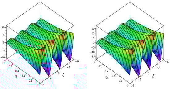
Figure 1. The first graph of analytical solution of $\beta =1$ and second is $\beta =0.8$ for Example 1.

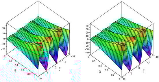
Figure 2. The first graph of analytical solution of $\beta =0.6$ and second is $\beta =0.4$ for Example 1.

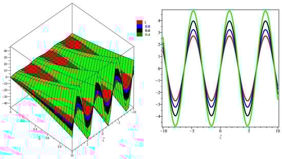
Figure 3. The different fractional-order of $\beta$ with respect to $\overline{\zeta }$ and $\overline{\Im }$ for Example 1.

Table 1. Example 1 Exact solution, proposed technique solutions and AE for $\rho (\overline{\zeta },\overline{\Im })$.

$\mathit{\kappa }=0.001$	Exact Solution	NDTM	AE of NDTM	AE of NDTM	AE of NDTM
$\mathbf{\gamma }$	$\mathbf{\beta }=\mathbf{1}$	$\mathbf{\beta }=\mathbf{1}$	$\mathbf{\beta }=\mathbf{1}$	$\mathbf{\beta }=\mathbf{0}.\mathbf{9}$	$\mathbf{\beta }=\mathbf{0}.\mathbf{8}$
0	0.000000000000	0.000000000000	0.0000000000$\times {10}^{+00}$	0.0000000000$\times {10}^{+00}$	0.0000000000$\times {10}^{+00}$
0.1	0.100000900000	0.100001000000	1.0000000000$\times {10}^{-7}$	2.2624000000$\times {10}^{-6}$	9.1005000000$\times {10}^{-6}$
0.2	0.200001600000	0.200002000000	4.0000000000$\times {10}^{-7}$	4.7247000000$\times {10}^{-6}$	1.8401000000$\times {10}^{-5}$
0.3	0.300002100000	0.300003000000	9.0000000000$\times {10}^{-7}$	7.3870000000$\times {10}^{-6}$	2.7901500000$\times {10}^{-5}$
0.4	0.400002400000	0.400004000000	1.6000000000$\times {10}^{-6}$	1.0249300000$\times {10}^{-5}$	3.7602000000$\times {10}^{-5}$
0.5	0.500002500000	0.500005000000	2.5000000000$\times {10}^{-6}$	1.3311600000$\times {10}^{-5}$	4.7502500000$\times {10}^{-5}$
0.6	0.600002400000	0.600006000000	3.6000000000$\times {10}^{-6}$	1.6574000000$\times {10}^{-5}$	5.7603000000$\times {10}^{-5}$
0.7	0.700002100000	0.700007000000	4.9000000000$\times {10}^{-6}$	2.0036200000$\times {10}^{-5}$	6.7903500000$\times {10}^{-5}$
0.8	0.800001600000	0.800008000000	6.4000000000$\times {10}^{-6}$	2.3698600000$\times {10}^{-5}$	7.8404000000$\times {10}^{-5}$
0.9	0.900000900000	0.900009000000	8.1000000000$\times {10}^{-6}$	2.7561000000$\times {10}^{-5}$	8.9104500000$\times {10}^{-5}$
1.0	1.000000000000	1.000010000000	1.0000000000$\times {10}^{-5}$	3.1624000000$\times {10}^{-5}$	1.0000500000$\times {10}^{-4}$

Example 2.

Consider the fractional-order linear Swift–Hohenberg equation:

$$\frac{{\partial }^{\beta }\rho (\overline{\zeta },\overline{\Im })}{\partial {\overline{\Im }}^{\beta }}+(1-\vartheta )\rho (\overline{\zeta },\overline{\Im })+2\frac{{\partial }^2\rho (\overline{\zeta },\overline{\Im })}{\partial {\overline{\zeta }}^2}+\frac{{\partial }^3\rho (\overline{\zeta },\overline{\Im })}{\partial {\overline{\zeta }}^3}=0,0<\beta \le 1,\overline{\Im }>0,$$

(39)

with initial condition

$$\rho (\overline{\zeta },0)=e^{\overline{\zeta }}.$$

(40)

Now, by considering the Natural transformation to Equation (39), we have

$$\mathcal{N}\left[\frac{{\partial }^{\beta }\rho (\overline{\zeta },\overline{\Im })}{\partial {\overline{\Im }}^{\beta }}\right]=-\mathcal{N}\left[(1-\vartheta )\rho (\overline{\zeta },\overline{\Im })+2\frac{{\partial }^2\rho (\overline{\zeta },\overline{\Im })}{\partial {\overline{\zeta }}^2}+\frac{{\partial }^3\rho (\overline{\zeta },\overline{\Im })}{\partial {\overline{\zeta }}^3}\right].$$

Applying the inverse Natural transformation

$$\rho (\overline{\zeta },\overline{\Im })={\mathcal{N}}^{-1}\left[\frac{{\mu }^2\rho (\overline{\zeta },0)}{s^2}-\frac{\mu (s+\beta (s-\mu \left)\right)}{s^2}\mathcal{N}\left[(1-\vartheta )\rho (\overline{\zeta },\overline{\Im })+2\frac{{\partial }^2\rho (\overline{\zeta },\overline{\Im })}{\partial {\overline{\zeta }}^2}+\frac{{\partial }^3\rho (\overline{\zeta },\overline{\Im })}{\partial {\overline{\zeta }}^3}\right]\right].$$

Applying the ADT procedure, we get

$${\rho }_0(\overline{\zeta },\overline{\Im })={\mathcal{N}}^{-1}\left[\frac{{\mu }^2\rho (\overline{\zeta },0)}{s^2}\right]={\mathcal{N}}^{-1}\left[\frac{{\mu }^2{e}^{\overline{\zeta }}}{s^2}\right]=e^{\overline{\zeta }}.$$

$${\rho }_{j+1}=-{\mathcal{N}}^{-1}\left[\frac{\mu (s+\beta (s-\mu \left)\right)}{s^2}\mathcal{N}\left\{(1-\vartheta ){\rho }_j(\overline{\zeta },\overline{\Im })+2\frac{{\partial }^2{\rho }_j(\overline{\zeta },\overline{\Im })}{\partial {\overline{\zeta }}^2}+\frac{{\partial }^3{\rho }_j(\overline{\zeta },\overline{\Im })}{\partial {\overline{\zeta }}^3}\right\}\right],j=0,1,2,\cdots$$

for $j=0$

$$\begin{array}{cc}\hfill & {\rho }_1(\overline{\zeta },\overline{\Im })=-{\mathcal{N}}^{-1}\left[\frac{\mu (s+\beta (s-\mu \left)\right)}{s^2}\mathcal{N}\left\{(1-\vartheta ){\rho }_0(\overline{\zeta },\overline{\Im })+2\frac{{\partial }^2{\rho }_0(\overline{\zeta },\overline{\Im })}{\partial {\overline{\zeta }}^2}+\frac{{\partial }^3{\rho }_0(\overline{\zeta },\overline{\Im })}{\partial {\overline{\zeta }}^3}\right\}\right]=(\vartheta -4)e^{\overline{\zeta }}(1-\beta +\beta \overline{\Im }).\hfill \end{array}$$

(41)

The subsequent terms read

$$\begin{array}{cc}\hfill {\rho }_2(\overline{\zeta },\overline{\Im })& =-{\mathcal{N}}^{-1}\left[\frac{\mu (s+\beta (s-\mu \left)\right)}{s^2}\mathcal{N}\left\{(1-\vartheta ){\rho }_1(\overline{\zeta },\overline{\Im })+2\frac{{\partial }^2{\rho }_1(\overline{\zeta },\overline{\Im })}{\partial {\overline{\zeta }}^2}+\frac{{\partial }^3{\rho }_1(\overline{\zeta },\overline{\Im })}{\partial {\overline{\zeta }}^3}\right\}\right]\hfill \\ \hfill & ={(\vartheta -4)}^2{e}^{\overline{\zeta }}\frac{1}{2}\overline{\Im }(\beta \overline{\Im }+2-2\beta ),\hfill \\ \hfill {\rho }_3(\overline{\zeta },\overline{\Im })& =-{\mathcal{N}}^{-1}\left[\frac{\mu (s+\beta (s-\mu \left)\right)}{s^2}\mathcal{N}\left\{(1-\vartheta ){\rho }_2(\overline{\zeta },\overline{\Im })+2\frac{{\partial }^2{\rho }_2(\overline{\zeta },\overline{\Im })}{\partial {\overline{\zeta }}^2}+\frac{{\partial }^3{\rho }_2(\overline{\zeta },\overline{\Im })}{\partial {\overline{\zeta }}^3}\right\}\right]\hfill \\ \hfill & ={(\vartheta -4)}^3{e}^{\overline{\zeta }}\frac{1}{3}{\overline{\Im }}^2(\beta \overline{\Im }+3-3\beta ),\hfill \\ \hfill & ⋮\hfill \end{array}$$

(42)

The NDM result for Example 2 is

$$\rho (\overline{\zeta },\overline{\Im })={\rho }_0(\overline{\zeta },\overline{\Im })+{\rho }_1(\overline{\zeta },\overline{\Im })+{\rho }_2(\overline{\zeta },\overline{\Im })+{\rho }_3(\overline{\zeta },\overline{\Im })+{\rho }_4(\overline{\zeta },\overline{\Im })\cdots .$$

$$\rho (\overline{\zeta },\overline{\Im })=e^{\overline{\zeta }}\left[1+(\vartheta -4)(1-\beta +\beta \overline{\Im })+{(\vartheta -4)}^2\frac{1}{2}\overline{\Im }(\beta \overline{\Im }+2-2\beta )+{(\vartheta -4)}^3\frac{1}{3}{\overline{\Im }}^2(\beta \overline{\Im }+3-3\beta )+\cdots \right].$$

when $\beta =1$, then the NDM result is

$$\rho (\overline{\zeta },\overline{\Im })=e^{\overline{\zeta }}\left[1+(\vartheta -4)e^{\overline{\zeta }}(1-\beta +\beta \overline{\Im })+{(\vartheta -4)}^2{e}^{\overline{\zeta }}\frac{1}{2}\overline{\Im }(\beta \overline{\Im }+2-2\beta )+{(\vartheta -4)}^3{e}^{\overline{\zeta }}\frac{1}{3}{\overline{\Im }}^2(\beta \overline{\Im }+3-3\beta )+\cdots \right].$$

(43)

The exact result is

$$\rho (\overline{\zeta },\overline{\Im })=e^{\overline{\zeta }}{E}_{\beta }\left((\vartheta -4){\overline{\Im }}^{\beta }\right).$$

Figure 4, demonstrates the close agreement between the exact and approximate solutions, which is a fascinating amalgamation of Natural transform and Caputo–Fabrizio fractional derivative for real parts only. Furthermore, Figure 5, depicts the fractional order behaviour of the real part of $\rho (\overline{\zeta },\overline{\Im })$ when fractional order $\beta =0.6$ and $0.4$, respectively. Figure 6, illustrates the three- and two-dimensional representations of various fractional-order of $\beta$. Table 2 shows that the comparison with the caputo and Caputo–Fabrizo operators.

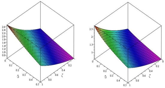
Figure 4. The first graph of analytical solution of $\beta =1$ and second is $\beta =0.8$ for Example 2.

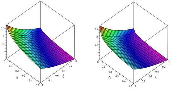
Figure 5. The first graph of analytical solution of $\beta =0.6$ and second is $\beta =0.4$ for Example 2.

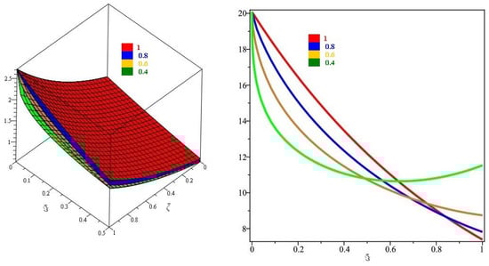
Figure 6. The different fractional-order of $\beta$ with respect to $\overline{\zeta }$ and $\overline{\Im }$ for Example 2.

Table 2. Comparison at different fractional-order of $\beta$ on the basis of error for Example 2.

$\overline{\mathit{\Im }}$	$\overline{\mathit{\zeta }}$	$\mathit{\beta }=0.4$	$\mathit{\beta }=0.6$	$\mathit{\beta }=0.8$	$\mathit{\beta }=1 \left({\mathbf{NDM}}_{\mathit{C}}\right)$	$\mathit{\beta }=1 \left({\mathbf{NDM}}_{\mathbf{CF}}\right)$
	0.2	5.2120000000 × 10${}^{-7}$	3.6017600000 × 10${}^{-7}$	2.0943200000 × 10${}^{-7}$	6.4513000000 × 10${}^{-8}$	6.4513000000 × 10${}^{-8}$
	0.4	1.0384330000 × 10${}^{-6}$	7.1776700000 × 10${}^{-7}$	4.1757400000 × 10${}^{-7}$	1.2893800000 × 10${}^{-7}$	1.2893800000 × 10${}^{-7}$
0.1	0.6	1.5474640000 × 10${}^{-6}$	1.0698980000 × 10${}^{-6}$	6.2282300000 × 10${}^{-7}$	1.9293900000 × 10${}^{-7}$	1.9293900000 × 10${}^{-7}$
	0.8	2.0443500000 × 10${}^{-6}$	1.4139470000 × 10${}^{-6}$	8.2379300000 × 10${}^{-7}$	2.5631800000 × 10${}^{-7}$	2.5631800000 × 10${}^{-7}$
	1	2.5253100000 × 10${}^{-6}$	1.7473930000 × 10${}^{-6}$	1.0191440000 × 10${}^{-6}$	3.1886900000 × 10${}^{-6}$	3.1886900000 × 10${}^{-6}$
	0.2	5.8984400000 × 10${}^{-7}$	4.2773700000 × 10${}^{-7}$	2.7455400000 × 10${}^{-7}$	1.2876600000 × 10${}^{-7}$	1.2876600000 × 10${}^{-7}$
	0.4	1.1759660000 × 10${}^{-6}$	8.5314400000 × 10${}^{-7}$	5.4809200000 × 10${}^{-7}$	2.5761600000 × 10${}^{-7}$	2.5761600000 × 10${}^{-7}$
0.2	0.6	1.7533840000 × 10${}^{-6}$	1.2726080000 × 10${}^{-6}$	8.1829600000 × 10${}^{-7}$	3.8562800000 × 10${}^{-7}$	3.8562800000 × 10${}^{-7}$
	0.8	2.3179040000 × 10${}^{-6}$	1.6832640000 × 10${}^{-6}$	1.0835570000 × 10${}^{-6}$	5.1239700000 × 10${}^{-7}$	5.1239700000 × 10${}^{-7}$
	1	2.8655420000 × 10${}^{-6}$	2.0823970000 × 10${}^{-6}$	1.3423590000 × 10${}^{-6}$	6.3748800000 × 10${}^{-7}$	6.3748800000 × 10${}^{-7}$
	0.2	6.5642700000 × 10${}^{-7}$	4.9400400000 × 10${}^{-7}$	3.3914500000 × 10${}^{-7}$	1.9276800000 × 10${}^{-7}$	1.9276800000 × 10${}^{-7}$
	0.4	1.3096920000 × 10${}^{-6}$	9.8624000000 × 10${}^{-7}$	6.7785000000 × 10${}^{-7}$	3.8605500000 × 10${}^{-7}$	3.8605500000 × 10${}^{-7}$
0.3	0.6	1.9537820000 × 10${}^{-6}$	1.4720680000 × 10${}^{-6}$	1.0127840000 × 10${}^{-6}$	5.7806700000 × 10${}^{-7}$	5.7806700000 × 10${}^{-7}$
	0.8	2.5842940000 × 10${}^{-6}$	1.9484160000 × 10${}^{-6}$	1.3421460000 × 10${}^{-6}$	7.6821500000 × 10${}^{-7}$	7.6821500000 × 10${}^{-7}$
	1	3.1969960000 × 10${}^{-6}$	2.4123230000 × 10${}^{-6}$	1.6641870000 × 10${}^{-6}$	9.5586800000 × 10${}^{-7}$	9.5586800000 × 10${}^{-7}$
	0.2	7.2188300000 × 10${}^{-7}$	5.5944200000 × 10${}^{-7}$	4.0328700000 × 10${}^{-7}$	2.5652100000 × 10${}^{-7}$	2.5652100000 × 10${}^{-7}$
	0.4	1.4414910000 × 10${}^{-6}$	1.1180020000 × 10${}^{-6}$	8.0703200000 × 10${}^{-7}$	5.1423300000 × 10${}^{-7}$	5.1423300000 × 10${}^{-7}$
0.4	0.6	2.1514870000 × 10${}^{-6}$	1.6697170000 × 10${}^{-6}$	1.2065920000 × 10${}^{-6}$	7.7025600000 × 10${}^{-7}$	7.7025600000 × 10${}^{-7}$
	0.8	2.8472250000 × 10${}^{-6}$	2.2112730000 × 10${}^{-6}$	1.5999330000 × 10${}^{-6}$	1.0237930000 × 10${}^{-6}$	1.0237930000 × 10${}^{-6}$
	1	3.5242520000 × 10${}^{-6}$	2.7394880000 × 10${}^{-6}$	1.9850950000 × 10${}^{-6}$	1.2740070000 × 10${}^{-6}$	1.2740070000 × 10${}^{-6}$
	0.2	7.8654200000 × 10${}^{-7}$	6.2423400000 × 10${}^{-7}$	4.6702100000 × 10${}^{-7}$	3.2001400000 × 10${}^{-7}$	3.2001400000 × 10${}^{-7}$
	0.4	1.5720280000 × 10${}^{-6}$	1.2488040000 × 10${}^{-6}$	9.3572800000 × 10${}^{-7}$	6.4215100000 × 10${}^{-7}$	6.4215100000 × 10${}^{-7}$
0.5	0.6	2.3474550000 × 10${}^{-6}$	1.8660800000 × 10${}^{-6}$	1.3998180000 × 10${}^{-6}$	9.6219500000 × 10${}^{-7}$	9.6219500000 × 10${}^{-7}$
	0.8	3.1079660000 × 10${}^{-6}$	2.4725350000 × 10${}^{-6}$	1.8570540000 × 10${}^{-6}$	1.2791210000 × 10${}^{-6}$	1.2791210000 × 10${}^{-6}$
	1	3.8489010000 × 10${}^{-6}$	3.0647790000 × 10${}^{-6}$	2.3052760000 × 10${}^{-6}$	1.5918960000 × 10${}^{-6}$	1.5918960000 × 10${}^{-6}$

Example 3.

Consider the fractional-order linear Swift–Hohenberg equation:

$$\frac{{\partial }^{\beta }\rho (\overline{\zeta },\overline{\Im })}{\partial {\overline{\Im }}^{\beta }}+(1-\vartheta )\rho (\overline{\zeta },\overline{\Im })+2\frac{{\partial }^2\rho (\overline{\zeta },\overline{\Im })}{\partial {\overline{\zeta }}^2}+\frac{{\partial }^4\rho (\overline{\zeta },\overline{\Im })}{\partial {\overline{\zeta }}^4}=0,0<\beta \le 1,\overline{\Im }>0,$$

(44)

with initial condition

$$\rho (\overline{\zeta },0)=cos\left(\overline{\zeta }\right).$$

(45)

Using the Natural transformation to Equation (44), we have

$$\mathcal{N}\left[\frac{{\partial }^{\beta }\rho (\overline{\zeta },\overline{\Im })}{\partial {\overline{\Im }}^{\beta }}\right]=-\mathcal{N}\left[(1-\vartheta )\rho (\overline{\zeta },\overline{\Im })+2\frac{{\partial }^2\rho (\overline{\zeta },\overline{\Im })}{\partial {\overline{\zeta }}^2}+\frac{{\partial }^4\rho (\overline{\zeta },\overline{\Im })}{\partial {\overline{\zeta }}^4}\right].$$

Applying the inverse Natural transformation

$$\rho (\overline{\zeta },\overline{\Im })={\mathcal{N}}^{-1}\left[\frac{{\mu }^2\rho (\overline{\zeta },0)}{s^2}-\frac{\mu (s+\beta (s-\mu \left)\right)}{s^2}\mathcal{N}\left\{(1-\vartheta )\rho (\overline{\zeta },\overline{\Im })+2\frac{{\partial }^2\rho (\overline{\zeta },\overline{\Im })}{\partial {\overline{\zeta }}^2}+\frac{{\partial }^4\rho (\overline{\zeta },\overline{\Im })}{\partial {\overline{\zeta }}^4}\right\}\right].$$

Applying the ADM procedure, we get

$${\rho }_0(\overline{\zeta },\overline{\Im })={\mathcal{N}}^{-1}\left[\frac{{\mu }^2\rho (\overline{\zeta },0)}{s^2}\right]={\mathcal{N}}^{-1}\left[\frac{{\mu }^{2}cos\left(\overline{\zeta }\right)}{s^2}\right]=cos\left(\overline{\zeta }\right),$$

$${\rho }_{j+1}=-{\mathcal{N}}^{-1}\left[\frac{\mu (s+\beta (s-\mu \left)\right)}{s^2}\mathcal{N}\left\{(1-\vartheta ){\rho }_j(\overline{\zeta },\overline{\Im })+2\frac{{\partial }^2{\rho }_j(\overline{\zeta },\overline{\Im })}{\partial {\overline{\zeta }}^2}+\frac{{\partial }^4{\rho }_j(\overline{\zeta },\overline{\Im })}{\partial {\overline{\zeta }}^4}\right\}\right],j=0,1,2,\cdots$$

(46)

The following two cases will be discussed.

Case 1: $(\vartheta =0)$. According to Equation (44), we get

for $j=0$

$$\begin{array}{cc}\hfill & {\rho }_1(\overline{\zeta },\overline{\Im })=-{\mathcal{N}}^{-1}\left[\frac{\mu (s+\beta (s-\mu \left)\right)}{s^2}\mathcal{N}\left\{(1-\vartheta ){\rho }_0(\overline{\zeta },\overline{\Im })+2\frac{{\partial }^2{\rho }_0(\overline{\zeta },\overline{\Im })}{\partial {\overline{\zeta }}^2}+\frac{{\partial }^4{\rho }_0(\overline{\zeta },\overline{\Im })}{\partial {\overline{\zeta }}^4}\right\}\right]=0.\hfill \end{array}$$

(47)

The subsequent terms read

$$\begin{array}{cc}\hfill & {\rho }_2(\overline{\zeta },\overline{\Im })=-{\mathcal{N}}^{-1}\left[\frac{\mu (s+\beta (s-\mu \left)\right)}{s^2}\mathcal{N}\left\{(1-\vartheta ){\rho }_1(\overline{\zeta },\overline{\Im })+2\frac{{\partial }^2{\rho }_1(\overline{\zeta },\overline{\Im })}{\partial {\overline{\zeta }}^2}+\frac{{\partial }^4{\rho }_1(\overline{\zeta },\overline{\Im })}{\partial {\overline{\zeta }}^4}\right\}\right]=0,\hfill \\ \hfill & {\rho }_3(\overline{\zeta },\overline{\Im })=-{\mathcal{N}}^{-1}\left[\frac{\mu (s+\beta (s-\mu \left)\right)}{s^2}\mathcal{N}\left\{(1-\vartheta ){\rho }_2(\overline{\zeta },\overline{\Im })+2\frac{{\partial }^2{\rho }_2(\overline{\zeta },\overline{\Im })}{\partial {\overline{\zeta }}^2}+\frac{{\partial }^4{\rho }_2(\overline{\zeta },\overline{\Im })}{\partial {\overline{\zeta }}^4}\right\}\right]=0,\hfill \\ \hfill & ⋮\hfill \end{array}$$

(48)

The Equation (44) solution is given as at $b=0$

$$\rho (\overline{\zeta },\overline{\Im })={\rho }_0(\overline{\zeta },\overline{\Im })+{\rho }_1(\overline{\zeta },\overline{\Im })+{\rho }_2(\overline{\zeta },\overline{\Im })+{\rho }_3(\overline{\zeta },\overline{\Im })+{\rho }_4(\overline{\zeta },\overline{\Im })\cdots .$$

$$\rho (\overline{\zeta },\overline{\Im })=cos\left(\overline{\zeta }\right).$$

Case 2: $(\vartheta \ne 0)$. According to Equation (44), we get

$${\rho }_0(\overline{\zeta },\overline{\Im })=cos\left(\overline{\zeta }\right).$$

In Equation (46) put $j=0,1,2,3\cdots$, is given as

$$\begin{array}{cc}\hfill & {\rho }_1(\overline{\zeta },\overline{\Im })=-{\mathcal{N}}^{-1}\left[\frac{\mu (s+\beta (s-\mu \left)\right)}{s^2}\mathcal{N}\left\{(1-\vartheta ){\rho }_0(\overline{\zeta },\overline{\Im })+2\frac{{\partial }^2{\rho }_0(\overline{\zeta },\overline{\Im })}{\partial {\overline{\zeta }}^2}+\frac{{\partial }^4{\rho }_0(\overline{\zeta },\overline{\Im })}{\partial {\overline{\zeta }}^4}\right\}\right],\hfill \\ \hfill & {\rho }_1(\overline{\zeta },\overline{\Im })=((\vartheta -1)+1)cos\left(\overline{\zeta }\right)(1-\beta +\beta \overline{\Im }).\hfill \end{array}$$

(49)

The subsequent terms read

$$\begin{array}{cc}\hfill & {\rho }_2(\overline{\zeta },\overline{\Im })=-{\mathcal{N}}^{-1}\left[\frac{\mu (s+\beta (s-\mu \left)\right)}{s^2}\mathcal{N}\left\{(1-\vartheta ){\rho }_1(\overline{\zeta },\overline{\Im })+2\frac{{\partial }^2{\rho }_1(\overline{\zeta },\overline{\Im })}{\partial {\overline{\zeta }}^2}+\frac{{\partial }^4{\rho }_1(\overline{\zeta },\overline{\Im })}{\partial {\overline{\zeta }}^4}\right\}\right],\hfill \\ \hfill & {\rho }_2(\overline{\zeta },\overline{\Im })=({(\vartheta -1)}^2+(\vartheta -1)+1)cos\left(\overline{\zeta }\right)\frac{1}{2}\overline{\Im }(\beta \overline{\Im }+2-2\beta ),\hfill \end{array}$$

(50)

$$\begin{array}{cc}\hfill & {\rho }_3(\overline{\zeta },\overline{\Im })=-{\mathcal{N}}^{-1}\left[\frac{\mu (s+\beta (s-\mu \left)\right)}{s^2}\mathcal{N}\left\{(1-\vartheta ){\rho }_2(\overline{\zeta },\overline{\Im })+2\frac{{\partial }^2{\rho }_2(\overline{\zeta },\overline{\Im })}{\partial {\overline{\zeta }}^2}+\frac{{\partial }^4{\rho }_2(\overline{\zeta },\overline{\Im })}{\partial {\overline{\zeta }}^4}\right\}\right],\hfill \\ \hfill & {\rho }_3(\overline{\zeta },\overline{\Im })=({(\vartheta -1)}^3+{(\vartheta -1)}^2+(\vartheta -1)+1)cos\left(\overline{\zeta }\right)\frac{1}{3}{\overline{\Im }}^2(\beta \overline{\Im }+3-3\beta ),\hfill \end{array}$$

(51)

$$\begin{array}{cc}\hfill & {\rho }_4(\overline{\zeta },\overline{\Im })=-{\mathcal{N}}^{-1}\left[\frac{\mu (s+\beta (s-\mu \left)\right)}{s^2}\mathcal{N}\left\{(1-\vartheta ){\rho }_3(\overline{\zeta },\overline{\Im })+2\frac{{\partial }^2{\rho }_3(\overline{\zeta },\overline{\Im })}{\partial {\overline{\zeta }}^2}+\frac{{\partial }^4{\rho }_3(\overline{\zeta },\overline{\Im })}{\partial {\overline{\zeta }}^4}\right\}\right],\hfill \\ \hfill & {\rho }_4(\overline{\zeta },\overline{\Im })=({(\vartheta -1)}^4+{(\vartheta -1)}^3+{(\vartheta -1)}^2+(\vartheta -1)+1)cos\left(\overline{\zeta }\right)\frac{1}{24}{\overline{\Im }}^3(\beta \overline{\Im }+4-4\beta ),\hfill \\ \hfill & ⋮\hfill \end{array}$$

(52)

The NDM result for Example 3 is given by

$$\rho (\overline{\zeta },\overline{\Im })={\rho }_0(\overline{\zeta },\overline{\Im })+{\rho }_1(\overline{\zeta },\overline{\Im })+{\rho }_2(\overline{\zeta },\overline{\Im })+{\rho }_3(\overline{\zeta },\overline{\Im })+{\rho }_4(\overline{\zeta },\overline{\Im })\cdots .$$

$$\begin{array}{cc}\hfill \rho (\overline{\zeta },\overline{\Im })& =cos\left(\overline{\zeta }\right)+((\vartheta -1)+1)cos\left(\overline{\zeta }\right)(1-\beta +\beta \overline{\Im })+({(\vartheta -1)}^2+(\vartheta -1)+1)cos\left(\overline{\zeta }\right)\frac{1}{2}\overline{\Im }(\beta \overline{\Im }+2-2\beta )\hfill \\ & +({(\vartheta -1)}^3+{(\vartheta -1)}^2+(\vartheta -1)+1)cos\left(\overline{\zeta }\right)\frac{1}{3}{\overline{\Im }}^2(\beta \overline{\Im }+3-3\beta )+({(\vartheta -1)}^4+{(\vartheta -1)}^3\hfill \\ & +{(\vartheta -1)}^2+(\vartheta -1)+1)cos\left(\overline{\zeta }\right)\frac{1}{24}{\overline{\Im }}^3(\beta \overline{\Im }+4-4\beta )+\cdots .\hfill \end{array}$$

The exact result for Equation (44) at $\beta =1$ reads

$$\rho (\overline{\zeta },\overline{\Im })=-\frac{1}{b}cos\left(\overline{\zeta }\right)\underset{N\to \infty }{lim}\sum _{n=0}^N(1-{(\vartheta -1)}^{n+1})(\beta \overline{\Im }+n-n\beta ).$$

(53)

Figure 7, demonstrates the close agreement between the exact and approximate solutions, which is a fascinating amalgamation of Natural transform and Caputo–Fabrizio fractional derivative for real parts only. Furthermore, Figure 8, depicts the fractional order behaviour of the real part of $\rho (\overline{\zeta },\overline{\Im })$ when fractional order $\beta =0.6$ and $0.4$, respectively. Figure 9, depicts the two-dimensional representation of various fractional-order of $\beta$ of Example 3.

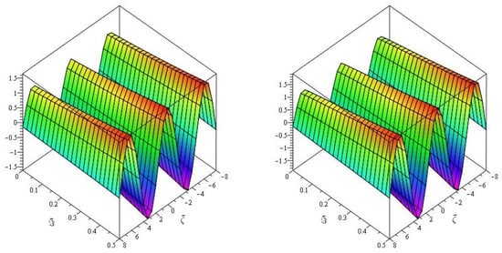
Figure 7. The first graph of analytical solution of $\beta =1$ and second is $\beta =0.8$ for Example 3.

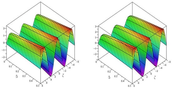
Figure 8. The first graph of analytical solution of $\beta =0.6$ and second is $\beta =0.4$ for Example 3.

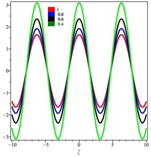
Figure 9. The different fractional-order of $\beta$ with respect to $\overline{\zeta }$ for Example 3.

Example 4.

Consider the fractional-order linear Swift–Hohenberg equation:

$$\frac{{\partial }^{\beta }\rho (\overline{\zeta },\overline{\Im })}{\partial {\overline{\Im }}^{\beta }}+(1-\vartheta )\rho (\overline{\zeta },\overline{\Im })+2\frac{{\partial }^2\rho (\overline{\zeta },\overline{\Im })}{\partial {\overline{\zeta }}^2}-\sigma \frac{{\partial }^3\rho (\overline{\zeta },\overline{\Im })}{\partial {\overline{\zeta }}^3}+\frac{{\partial }^4\rho (\overline{\zeta },\overline{\Im })}{\partial {\overline{\zeta }}^4}=0,0<\beta \le 1,\overline{\Im }>0,$$

(54)

with initial condition

$$\rho (\overline{\zeta },0)=e^{\overline{\zeta }}.$$

(55)

Now, by applying the Natural transform to Equation (54), we get

$$\mathcal{N}\left[\frac{{\partial }^{\beta }\rho (\overline{\zeta },\overline{\Im })}{\partial {\overline{\Im }}^{\beta }}\right]=-\mathcal{N}\left[(1-\vartheta )\rho (\overline{\zeta },\overline{\Im })+2\frac{{\partial }^2\rho (\overline{\zeta },\overline{\Im })}{\partial {\overline{\zeta }}^2}-\sigma \frac{{\partial }^3\rho (\overline{\zeta },\overline{\Im })}{\partial {\overline{\zeta }}^3}+\frac{{\partial }^4\rho (\overline{\zeta },\overline{\Im })}{\partial {\overline{\zeta }}^4}\right].$$

Applying the inverse Natural transformation

$$\rho (\overline{\zeta },\overline{\Im })={\mathcal{N}}^{-1}\left[\frac{{\mu }^2\rho (\overline{\zeta },0)}{s}-\frac{\mu (s+\beta (s-\mu \left)\right)}{s^2}\mathcal{N}\left\{(1-\vartheta )\rho (\overline{\zeta },\overline{\Im })+2\frac{{\partial }^2\rho (\overline{\zeta },\overline{\Im })}{\partial {\overline{\zeta }}^2}-\sigma \frac{{\partial }^3\rho (\overline{\zeta },\overline{\Im })}{\partial {\overline{\zeta }}^3}+\frac{{\partial }^4\rho (\overline{\zeta },\overline{\Im })}{\partial {\overline{\zeta }}^4}\right\}\right].$$

Using the ADT procedure, we get:

$${\rho }_0(\overline{\zeta },\overline{\Im })={\mathcal{N}}^{-1}\left[\frac{{\mu }^2\rho (\overline{\zeta },0)}{s^2}\right]={\mathcal{N}}^{-1}\left[\frac{{\mu }^2{e}^{\overline{\zeta }}}{s^2}\right]=e^{\overline{\zeta }}.$$

$${\rho }_{j+1}=-{\mathcal{N}}^{-1}\left[\frac{\mu (s+\beta (s-\mu \left)\right)}{s^2}\mathcal{N}\left\{(1-\vartheta ){\rho }_j(\overline{\zeta },\overline{\Im })+2\frac{{\partial }^2{\rho }_j(\overline{\zeta },\overline{\Im })}{\partial {\overline{\zeta }}^2}-\sigma \frac{{\partial }^3{\rho }_j(\overline{\zeta },\overline{\Im })}{\partial {\overline{\zeta }}^3}+\frac{{\partial }^4{\rho }_j(\overline{\zeta },\overline{\Im })}{\partial {\overline{\zeta }}^4}\right\}\right],j=0,1,2,\cdots$$

for $j=0$

$$\begin{array}{cc}\hfill & {\rho }_1(\overline{\zeta },\overline{\Im })=-{\mathcal{N}}^{-1}\left[\frac{\mu (s+\beta (s-\mu \left)\right)}{s^2}\mathcal{N}\left\{(1-\vartheta ){\rho }_0(\overline{\zeta },\overline{\Im })+2\frac{{\partial }^2{\rho }_0(\overline{\zeta },\overline{\Im })}{\partial {\overline{\zeta }}^2}-\sigma \frac{{\partial }^3{\rho }_0(\overline{\zeta },\overline{\Im })}{\partial {\overline{\zeta }}^3}+\frac{{\partial }^4{\rho }_0(\overline{\zeta },\overline{\Im })}{\partial {\overline{\zeta }}^4}\right\}\right],\hfill \\ \hfill & {\rho }_1(\overline{\zeta },\overline{\Im })=(\vartheta -4+\sigma )e^{\overline{\zeta }}(1-\beta +\beta \overline{\Im }).\hfill \end{array}$$

(56)

The subsequent terms read

$$\begin{array}{cc}\hfill & {\rho }_2(\overline{\zeta },\overline{\Im })=-{\mathcal{N}}^{-1}\left[\frac{\mu (s+\beta (s-\mu \left)\right)}{s^2}\mathcal{N}\left\{(1-\vartheta ){\rho }_1(\overline{\zeta },\overline{\Im })+2\frac{{\partial }^2{\rho }_1(\overline{\zeta },\overline{\Im })}{\partial {\overline{\zeta }}^2}-\sigma \frac{{\partial }^3{\rho }_1(\overline{\zeta },\overline{\Im })}{\partial {\overline{\zeta }}^3}+\frac{{\partial }^4{\rho }_1(\overline{\zeta },\overline{\Im })}{\partial {\overline{\zeta }}^4}\right\}\right],\hfill \\ \hfill & {\rho }_2(\overline{\zeta },\overline{\Im })={(\vartheta -4+\sigma )}^2{e}^{\overline{\zeta }}\frac{1}{2}\overline{\Im }(\beta \overline{\Im }+2-2\beta ),\hfill \\ \hfill & {\rho }_3(\overline{\zeta },\overline{\Im })=-{\mathcal{N}}^{-1}\left[\frac{\mu (s+\beta (s-\mu \left)\right)}{s^2}\mathcal{N}\left\{(1-\vartheta ){\rho }_2(\overline{\zeta },\overline{\Im })+2\frac{{\partial }^2{\rho }_2(\overline{\zeta },\overline{\Im })}{\partial {\overline{\zeta }}^2}-\sigma \frac{{\partial }^3{\rho }_2(\overline{\zeta },\overline{\Im })}{\partial {\overline{\zeta }}^3}+\frac{{\partial }^4{\rho }_2(\overline{\zeta },\overline{\Im })}{\partial {\overline{\zeta }}^4}\right\}\right],\hfill \\ \hfill & {\rho }_3(\overline{\zeta },\overline{\Im })={(\vartheta -4+\sigma )}^3{e}^{\overline{\zeta }}\frac{1}{3}{\overline{\Im }}^2(\beta \overline{\Im }+3-3\beta ),\hfill \\ \hfill & ⋮\hfill \end{array}$$

(57)

The NDM result for Example 4 is given by

$$\rho (\overline{\zeta },\overline{\Im })={\rho }_0(\overline{\zeta },\overline{\Im })+{\rho }_1(\overline{\zeta },\overline{\Im })+{\rho }_2(\overline{\zeta },\overline{\Im })+{\rho }_3(\overline{\zeta },\overline{\Im })+{\rho }_4(\overline{\zeta },\overline{\Im })\cdots .$$

$$\rho (\overline{\zeta },\overline{\Im })=e^{\overline{\zeta }}\left[1+(\vartheta -4)(1-\beta +\beta \overline{\Im })+{(\vartheta -4)}^2\frac{1}{2}\overline{\Im }(\beta \overline{\Im }+2-2\beta )+{(\vartheta -4)}^3\frac{1}{3}{\overline{\Im }}^2(\beta \overline{\Im }+3-3\beta )+\cdots \right].$$

when $\beta =1$, then the NDM result is

$$\rho (\overline{\zeta },\overline{\Im })=e^{\overline{\zeta }}\left[1+(\vartheta -4+\sigma )(1-\beta +\beta \overline{\Im })+{(\vartheta -4+\sigma )}^2\frac{1}{2}\overline{\Im }(\beta \overline{\Im }+2-2\beta )+{(\vartheta -4+\sigma )}^3\frac{1}{3}{\overline{\Im }}^2(\beta \overline{\Im }+3-3\beta )+\cdots \right].$$

(58)

The exact result reads

$$\rho (\overline{\zeta },\overline{\Im })={exp}^{\overline{\zeta }}{E}_{\beta }\left((\vartheta -4+\sigma ){\overline{\Im }}^{\beta }\right).$$

Figure 10, demonstrates the close agreement between the exact and approximate solutions, which is a fascinating amalgamation of Natural transform and Caputo–Fabrizio fractional derivative for real parts only. Furthermore, Figure 11, depicts the fractional order behaviour of the real part of $\rho (\overline{\zeta },\overline{\Im })$ when fractional order $\beta =0.6$ and $0.4$, respectively of Example 4.

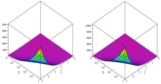
Figure 10. The first graph of analytical solution of $\beta =1$ and second is $\beta =0.8$ for Example 3.

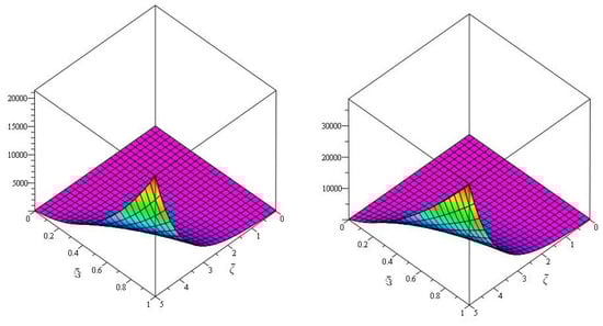
Figure 11. The first graph of analytical solution of $\beta =0.6$ and second is $\beta =0.4$ for Example 3.

Example 5.

Consider the fractional-order non-linear Swift–Hohenberg equation:

$$\frac{{\partial }^{\beta }\rho (\overline{\zeta },\overline{\Im })}{\partial {\overline{\Im }}^{\beta }}+(1-\vartheta )\rho (\overline{\zeta },\overline{\Im })+2\frac{{\partial }^2\rho (\overline{\zeta },\overline{\Im })}{\partial {\overline{\zeta }}^2}+\frac{{\partial }^4\rho (\overline{\zeta },\overline{\Im })}{\partial {\overline{\zeta }}^4}-{\rho }^2(\overline{\zeta },\overline{\Im })+{\left(\frac{\partial \rho (\overline{\zeta },\overline{\Im })}{\partial \overline{\zeta }}\right)}^2=0,0<\beta \le 1,\overline{\Im }>0,$$

(59)

with initial condition

$$\rho (\overline{\zeta },0)=e^{\overline{\zeta }}.$$

(60)

Using the Natural transformation to Equation (59), we get

$$\mathcal{N}\left[\frac{{\partial }^{\beta }\rho (\overline{\zeta },\overline{\Im })}{\partial {\overline{\Im }}^{\beta }}\right]=-\mathcal{N}\left[(1-\vartheta )\rho (\overline{\zeta },\overline{\Im })+2\frac{{\partial }^2\rho (\overline{\zeta },\overline{\Im })}{\partial {\overline{\zeta }}^2}+\frac{{\partial }^4\rho (\overline{\zeta },\overline{\Im })}{\partial {\overline{\zeta }}^4}-{\rho }^2(\overline{\zeta },\overline{\Im })+{\left(\frac{\partial \rho (\overline{\zeta },\overline{\Im })}{\partial \overline{\zeta }}\right)}^2\right].$$

Applying the inverse Natural transformation

$$\begin{array}{cc}\hfill \rho (\overline{\zeta },\overline{\Im })=& {\mathcal{N}}^{-1}\left[\frac{{\mu }^2\rho (\overline{\zeta },0)}{s^2}-\frac{\mu (s+\beta (s-\mu \left)\right)}{s^2}\mathcal{N}\left\{(1-\vartheta )\rho (\overline{\zeta },\overline{\Im })+2\frac{{\partial }^2\rho (\overline{\zeta },\overline{\Im })}{\partial {\overline{\zeta }}^2}+\frac{{\partial }^4\rho (\overline{\zeta },\overline{\Im })}{\partial {\overline{\zeta }}^4}\right.\right.\hfill \\ & \left.\left.-{\rho }^2(\overline{\zeta },\overline{\Im })+{\left(\frac{\partial \rho (\overline{\zeta },\overline{\Im })}{\partial \overline{\zeta }}\right)}^2\right\}\right].\hfill \end{array}$$

Using the ADT procedure, we get

$${\rho }_0(\overline{\zeta },\overline{\Im })={\mathcal{N}}^{-1}\left[\frac{{\mu }^2\rho (\overline{\zeta },0)}{s^2}\right]={\mathcal{N}}^{-1}\left[\frac{{\mu }^2{e}^{\overline{\zeta }}}{s^2}\right]=e^{\overline{\zeta }}.$$

$${\rho }_{j+1}=-{\mathcal{N}}^{-1}\left[\frac{\mu (s+\beta (s-\mu \left)\right)}{s^2}\mathcal{N}\left\{(1-\vartheta )\rho (\overline{\zeta },\overline{\Im })-2\frac{{\partial }^2\rho (\overline{\zeta },\overline{\Im })}{\partial {\overline{\zeta }}^2}-\frac{{\partial }^4\rho (\overline{\zeta },\overline{\Im })}{\partial {\overline{\zeta }}^4}+\sum _{m=0}^{\infty }{\mathcal{A}}_m-\sum _{m=0}^{\infty }{\mathcal{B}}_m\right\}\right],j=0,1,2,\cdots$$

The nonlinear term can be with the help of Adomian polynomials is expressed as,

$$\begin{array}{cc}\hfill & {\mathcal{A}}_0={\rho }_0^2,{\mathcal{A}}_1=2{\rho }_0{\rho }_1,\hfill \\ \hfill & {\mathcal{B}}_0={\left({\rho }_{0\overline{\zeta }}\right)}^2,{\mathcal{B}}_1=2{\rho }_{0\overline{\zeta }}{\rho }_{1\overline{\zeta }},\hfill \end{array}$$

for $j=0$

$$\begin{array}{cc}\hfill & {\rho }_1(\overline{\zeta },\overline{\Im })=-{\mathcal{N}}^{-1}\left[\frac{\mu (s+\beta (s-\mu \left)\right)}{s^2}\mathcal{N}\left\{(1-\vartheta ){\rho }_0(\overline{\zeta },\overline{\Im })+2\frac{{\partial }^2{\rho }_0(\overline{\zeta },\overline{\Im })}{\partial {\overline{\zeta }}^2}+\frac{{\partial }^4{\rho }_0(\overline{\zeta },\overline{\Im })}{\partial {\overline{\zeta }}^4}-{\rho }^2(\overline{\zeta },\overline{\Im })+{\left(\frac{\partial {\rho }_0(\overline{\zeta },\overline{\Im })}{\partial \overline{\zeta }}\right)}^2\right\}\right],\hfill \\ \hfill & {\rho }_1(\overline{\zeta },\overline{\Im })=(\vartheta -4)e^{\overline{\zeta }}(1-\beta +\beta \overline{\Im }).\hfill \end{array}$$

(61)

The subsequent terms read

$$\begin{array}{cc}\hfill & {\rho }_2(\overline{\zeta },\overline{\Im })={(\vartheta -4)}^2{e}^{\overline{\zeta }}\frac{1}{2}\overline{\Im }(\beta \overline{\Im }+2-2\beta ),\hfill \\ \hfill & {\rho }_3(\overline{\zeta },\overline{\Im })={(\vartheta -4)}^3{e}^{\overline{\zeta }}\frac{1}{3}{\overline{\Im }}^2(\beta \overline{\Im }+3-3\beta ),\hfill \\ \hfill & ⋮\hfill \end{array}$$

(62)

The NDM result for Example 5 is given by

$$\rho (\overline{\zeta },\overline{\Im })={\rho }_0(\overline{\zeta },\overline{\Im })+{\rho }_1(\overline{\zeta },\overline{\Im })+{\rho }_2(\overline{\zeta },\overline{\Im })+{\rho }_3(\overline{\zeta },\overline{\Im })+{\rho }_4(\overline{\zeta },\overline{\Im })\cdots .$$

$$\rho (\overline{\zeta },\overline{\Im })=e^{\overline{\zeta }}\left[1+(\vartheta -4)(1-\beta +\beta \overline{\Im })+{(\vartheta -4)}^2\frac{1}{2}\overline{\Im }(\beta \overline{\Im }+2-2\beta )+{(\vartheta -4)}^3\frac{1}{3}{\overline{\Im }}^2(\beta \overline{\Im }+3-3\beta )+\cdots \right].$$

The exact result reads

$$\rho (\overline{\zeta },\overline{\Im })=e^{\overline{\zeta }}{E}_{\beta }\left((\vartheta -4){\overline{\Im }}^{\beta }\right).$$

Example 6.

Consider the fractional-order non-linear Swift–Hohenberg equation:

$$\begin{array}{cc}\hfill \frac{{\partial }^{\beta }\rho (\overline{\zeta },\overline{\Im })}{\partial {\overline{\Im }}^{\beta }}& +(1-\vartheta )\rho (\overline{\zeta },\overline{\Im })+2\frac{{\partial }^2\rho (\overline{\zeta },\overline{\Im })}{\partial {\overline{\zeta }}^2}-\sigma \frac{{\partial }^3\rho (\overline{\zeta },\overline{\Im })}{\partial {\overline{\zeta }}^3}\hfill \\ \hfill & +\frac{{\partial }^4\rho (\overline{\zeta },\overline{\Im })}{\partial {\overline{\zeta }}^4}-{\rho }^2(\overline{\zeta },\overline{\Im })+{\left(\frac{\partial \rho (\overline{\zeta },\overline{\Im })}{\partial \overline{\zeta }}\right)}^2=0,0<\beta \le 1,\overline{\Im }>0,\hfill \end{array}$$

(63)

with initial condition

$$\rho (\overline{\zeta },0)=e^{\overline{\zeta }},$$

(64)

Now, by applying the Natural transformation to Equation (59), we get

$$\mathcal{N}\left[\frac{{\partial }^{\beta }\rho (\overline{\zeta },\overline{\Im })}{\partial {\overline{\Im }}^{\beta }}\right]=-\mathcal{N}\left[(1-\vartheta )\rho (\overline{\zeta },\overline{\Im })+2\frac{{\partial }^2\rho (\overline{\zeta },\overline{\Im })}{\partial {\overline{\zeta }}^2}-\sigma \frac{{\partial }^3\rho (\overline{\zeta },\overline{\Im })}{\partial {\overline{\zeta }}^3}+\frac{{\partial }^4\rho (\overline{\zeta },\overline{\Im })}{\partial {\overline{\zeta }}^4}-{\rho }^2(\overline{\zeta },\overline{\Im })+{\left(\frac{\partial \rho (\overline{\zeta },\overline{\Im })}{\partial \overline{\zeta }}\right)}^2\right],$$

Applying the inverse Natural transformation

$$\begin{array}{cc}\hfill \rho (\overline{\zeta },\overline{\Im })& ={\mathcal{N}}^{-1}\left[\frac{{\mu }^2\rho (\overline{\zeta },0)}{s^2}-\frac{\mu (s+\beta (s-\mu \left)\right)}{s^2}\mathcal{N}\left[(1-\vartheta )\rho (\overline{\zeta },\overline{\Im })+2\frac{{\partial }^2\rho (\overline{\zeta },\overline{\Im })}{\partial {\overline{\zeta }}^2}-\sigma \frac{{\partial }^3\rho (\overline{\zeta },\overline{\Im })}{\partial {\overline{\zeta }}^3}\right.\right.\hfill \\ & \left.\left.+\frac{{\partial }^4\rho (\overline{\zeta },\overline{\Im })}{\partial {\overline{\zeta }}^4}-{\rho }^2(\overline{\zeta },\overline{\Im })+{\left(\frac{\partial \rho (\overline{\zeta },\overline{\Im })}{\partial \overline{\zeta }}\right)}^2\right]\right].\hfill \end{array}$$

Using the ADT procedure, we get

$${\rho }_0(\overline{\zeta },\overline{\Im })={\mathcal{N}}^{-1}\left[\frac{{\mu }^2\rho (\overline{\zeta },0)}{s^2}\right]={\mathcal{N}}^{-1}\left[\frac{{\mu }^2{e}^{\overline{\zeta }}}{s^2}\right]=e^{\overline{\zeta }}.$$

$${\rho }_{j+1}=-{\mathcal{N}}^{-1}\left[\frac{\mu (s+\beta (s-\mu \left)\right)}{s^2}\mathcal{N}\left\{(1-\vartheta )\rho (\overline{\zeta },\overline{\Im })-2\frac{{\partial }^2\rho (\overline{\zeta },\overline{\Im })}{\partial {\overline{\zeta }}^2}+\sigma \frac{{\partial }^3\rho (\overline{\zeta },\overline{\Im })}{\partial {\overline{\zeta }}^3}-\frac{{\partial }^4\rho (\overline{\zeta },\overline{\Im })}{\partial {\overline{\zeta }}^4}+\sum _{m=0}^{\infty }{\mathcal{A}}_m-\sum _{m=0}^{\infty }{\mathcal{B}}_m\right\}\right].$$

The nonlinear term can be defined with the help of Adomian polynomials as

$$\begin{array}{cc}\hfill & {\mathcal{A}}_0={\rho }_0^2,{\mathcal{A}}_1=2{\rho }_0{\rho }_1,\hfill \\ \hfill & {\mathcal{B}}_0={\left({\rho }_{0\overline{\zeta }}\right)}^2,{\mathcal{B}}_1=2{\rho }_{0\overline{\zeta }}{\rho }_{1\overline{\zeta }},\hfill \end{array}$$

for $j=0$

$$\begin{array}{cc}\hfill {\rho }_1(\overline{\zeta },\overline{\Im })=& -{\mathcal{N}}^{-1}\left[\frac{\mu (s+\beta (s-\mu \left)\right)}{s^2}\mathcal{N}\left\{(1-\vartheta ){\rho }_0(\overline{\zeta },\overline{\Im })+2\frac{{\partial }^2{\rho }_0(\overline{\zeta },\overline{\Im })}{\partial {\overline{\zeta }}^2}-\sigma \frac{{\partial }^3{\rho }_0(\overline{\zeta },\overline{\Im })}{\partial {\overline{\zeta }}^3}\right.\right.\hfill \\ \hfill & \left.\left.+\frac{{\partial }^4{\rho }_0(\overline{\zeta },\overline{\Im })}{\partial {\overline{\zeta }}^4}-{\rho }_0^2(\overline{\zeta },\overline{\Im })+{\left(\frac{\partial {\rho }_0(\overline{\zeta },\overline{\Im })}{\partial \overline{\zeta }}\right)}^2\right\}\right]=(\vartheta -4+\sigma )e^{\overline{\zeta }}(1-\beta +\beta \overline{\Im }).\hfill \end{array}$$

(65)

The subsequent terms read

$$\begin{array}{cc}\hfill & {\rho }_2(\overline{\zeta },\overline{\Im })={(\vartheta -4+\sigma )}^2{e}^{\overline{\zeta }}\frac{1}{2}\overline{\Im }(\beta \overline{\Im }+2-2\beta ),\hfill \\ \hfill & {\rho }_3(\overline{\zeta },\overline{\Im })={(\vartheta -4+\sigma )}^3{e}^{\overline{\zeta }}\frac{1}{3}{\overline{\Im }}^2(\beta \overline{\Im }+3-3\beta ),\hfill \\ \hfill & ⋮\hfill \end{array}$$

(66)

The NDM result for Example 6 is given by

$$\rho (\overline{\zeta },\overline{\Im })={\rho }_0(\overline{\zeta },\overline{\Im })+{\rho }_1(\overline{\zeta },\overline{\Im })+{\rho }_2(\overline{\zeta },\overline{\Im })+{\rho }_3(\overline{\zeta },\overline{\Im })+{\rho }_4(\overline{\zeta },\overline{\Im })\cdots$$

$$\rho (\overline{\zeta },\overline{\Im })=e^{\overline{\zeta }}\left[1+(\vartheta -4+\sigma )(1-\beta +\beta \overline{\Im })+{(\vartheta -4+\sigma )}^2\frac{1}{2}\overline{\Im }(\beta \overline{\Im }+2-2\beta )+{(\vartheta -4+\sigma )}^3\frac{1}{3}{\overline{\Im }}^2(\beta \overline{\Im }+3-3\beta )+\cdots \right].$$

The exact result reads

$$\rho (\overline{\zeta },\overline{\Im })=e^{\overline{\zeta }}{E}_{\beta }\left((\vartheta -4+\sigma ){\overline{\Im }}^{\beta }\right).$$

6. Conclusions

In this investigation, a novel technique known as Natural decomposition has been devoted to obtain the fractional-order analytical result to Swift–Hohenberg equation. By applying the later technique, we studied a fractional-order (non)linear Swift–Hohenberg equation involving and excluding dispersive terms. We compared the solutions using figures for the various fractional-orders. After that, we studied the problem described above under Caputo–Fabrizio fractional-order derivative. The obtained solutions can be helpful for further analysis of the complicated nonlinear physical models. The calculations of this method are very simple and straightforward. Thus, we deduced that this method can be applied to solve different systems of nonlinear fractional-order partial differential equations. In addition, the suggested method can be used for solving many nonlinear evolution equations that govern the propagation of unmodulated and modulated structures in different plasma systems. For instance, this method can be employed for solving the family of fractional Kawahara-type equations that govern the propagation of strong nonlinear unmodulated structures in a plasma physics [32,33,34]. Finally, we can conclude the regarded technique is better and highly effective, and it can be utilized to study the various classes of nonlinear problems arisen in real life.

References

- Sabatier, J.A.T.M.J.; Agrawal, O.P.; Machado, J.T. Advances in Fractional Calculus; Springer: Dordrecht, The Netherlands, 2007; Volume 4. [Google Scholar]
- Atangana, A.; Baleanu, D. Caputo–Fabrizio derivative applied to groundwater flow within confined aquifer. J. Eng. Mech. 2017, 143, D4016005. [Google Scholar] [CrossRef]
- Aljahdaly, N.H.; Agarwal, R.P.; Botmart, T. The analysis of the fractional-order system of third-order KdV equation within different operators. Alex. Eng. J. 2022, 61, 11825–11834. [Google Scholar] [CrossRef]
- Mukhtar, S.; Noor, S. The Numerical Investigation of a Fractional-Order Multi-Dimensional Model of Navier-Stokes Equation via Novel Techniques. Symmetry 2022, 14, 1102. [Google Scholar] [CrossRef]
- Morales-Delgado, V.F.; Gómez-Aguilar, J.F.; Yépez-Martínez, H.; Baleanu, D.; Escobar-Jimenez, R.F.; Olivares-Peregrino, V.H. Laplace homotopy analysis method for solving linear partial differential equations using a fractional derivative with and without kernel singular. Adv. Differ. Equ. 2016, 2016, 164. [Google Scholar] [CrossRef]
- Li, Y.; Nohara, B.T.; Liao, S. Series solutions of coupled Van der Pol equation by means of homotopy analysis method. J. Math. Phys. 2010, 51, 063517. [Google Scholar] [CrossRef]
- Shah, R.; Khan, H.; Baleanu, D. Fractional Whitham-Broer-Kaup Equations within Modified Analytical Approaches. Axioms 2019, 8, 125. [Google Scholar] [CrossRef]
- El-Tantawy, S.A.; Shan, S.A.; Mustafa, N.; Alshehri, M.H.; Duraihem, F.Z.; Turki, N.B. Homotopy perturbation and Adomian decomposition methods for modeling the nonplanar structures in a bi-ion ionospheric superthermal plasma. Eur. Phys. J. Plus 2021, 136, 561. [Google Scholar] [CrossRef]
- Kashkari, B.S.; El-Tantawy, S.A.; Salas, A.H.; El-Sherif, L.S. Homotopy perturbation method for studying dissipative nonplanar solitons in an electronegative complex plasma. Chaos Solitons Fractals 2020, 130, 109457. [Google Scholar] [CrossRef]
- Alshehry, A.S.; Imran, M.; Weera, W. Fractional-View Analysis of Fokker-Planck Equations by ZZ Transform with Mittag-Leffler Kernel. Symmetry 2022, 14, 1513. [Google Scholar] [CrossRef]
- Wu, S. Nonlinear information data mining based on time series for fractional differential operators. Chaos Interdiscip. J. Nonlinear Sci. 2019, 29, 013114. [Google Scholar] [CrossRef]
- Lakshmikantham, V.; Vatsala, A.S. Basic theory of fractional differential equations. Nonlinear Anal. Theory Methods Appl. 2008, 69, 2677–2682. [Google Scholar] [CrossRef]
- Prakasha, D.G.; Veeresha, P.; Baskonus, H.M. Residual power series method for fractional Swift–Hohenberg equation. Fractal Fract. 2019, 3, 9. [Google Scholar] [CrossRef]
- Swift, J.; Hohenberg, P.C. Hydrodynamics fluctuations at the convective instability. Phys. Rev. A 1977, 15, 319–328. [Google Scholar] [CrossRef]
- Lega, L.; Moloney, J.V.; Newell, A.C. Swift–Hohenberg equation for lasers. Phys. Rev. Lett. 1994, 73, 2978–2981. [Google Scholar] [CrossRef]
- Pomeau, Y.; Zaleski, S. Dislocation motion in cellular structures. Phys. Rev. A 1983, 27, 2710–2726. [Google Scholar] [CrossRef]
- Peletier, L.A.; Rottschafer, V. Large time behaviour of solutions of the SwiftHohenberg equation. R. Acad. Sci. Paris Ser. I 2003, 336, 225–230. [Google Scholar] [CrossRef]
- Ahmadian, A.; Ismail, F.; Salahshour, S.; Baleanu, D.; Ghaemi, F. Uncertain viscoelastic models with fractional order: A new spectral tau method to study the numerical simulations of the solution. Commun. Nonlinear Sci. Numer. Simul. 2017, 53, 44–64. [Google Scholar] [CrossRef]
- Fife, P.C. Pattern formation in gradient systems. In Handbook of Dynamical Systems; Esevier: Amsterdam, The Netherlands, 2002; Volume 2, pp. 679–719. [Google Scholar]
- Hoyle, R.B. Pattern Formation; Cambridge University Press: Cambridge, UK, 2006. [Google Scholar]
- Ryabov, P.N.; Kudryashov, N.A. Nonlinear waves described by the generalized Swift–Hohenberg equation. J. Phys. Conf. Ser. 2017, 788, 012032. [Google Scholar] [CrossRef]
- Vishal, K.; Kumar, S.; Das, S. Application of homotopy analysis method for fractional Swift Hohenberg equation—Revisited. Appl. Math. Model. 2012, 36, 3630–3637. [Google Scholar] [CrossRef]
- Khan, N.A.; Khan, N.U.; Ayaz, M.; Mahmood, A. Analytical methods for solving the time-fractional Swift–Hohenberg (S-H) equation. Comput. Math. Appl. 2011, 61, 2181–2185. [Google Scholar] [CrossRef]
- Li, W.; Pang, Y. An iterative method for time-fractional Swift–Hohenberg equation. Adv. Math. Phys. 2018, 2018, 2405432. [Google Scholar] [CrossRef]
- Vishal, K.; Das, S.; Ong, S.H.; Ghosh, P. On the solutions of fractional Swift Hohenberg equation with dispersion. Appl. Math. Comput. 2013, 219, 5792–5801. [Google Scholar] [CrossRef]
- Rawashdeh, M.S.; Al-Jammal, H. New approximate solutions to fractional nonlinear systems of partial differential equations using the FNDM. Adv. Differ. Equ. 2016, 2016, 235. [Google Scholar] [CrossRef]
- Rawashdeh, M.S.; Al-Jammal, H. Numerical solutions for systems of nonlinear fractional ordinary differential equations using the FNDM. Mediterr. J. Math. 2016, 13, 4661–4677. [Google Scholar] [CrossRef]
- Rawashdeh, M.S. The fractional natural decomposition method: Theories and applications. Math. Methods Appl. Sci. 2017, 40, 2362–2376. [Google Scholar] [CrossRef]
- Aljahdaly, N.H.; Akgul, A.; Shah, R.; Mahariq, I.; Kafle, J. A comparative analysis of the fractional-order coupled Korteweg-De Vries equations with the Mittag-Leffler law. J. Math. 2022, 2022, 8876149. [Google Scholar] [CrossRef]
- Shah, N.A.; Hamed, Y.S.; Abualnaja, K.M.; Chung, J.D.; Shah, R.; Khan, A. A comparative analysis of fractional-order kaup-kupershmidt equation within different operators. Symmetry 2022, 14, 986. [Google Scholar] [CrossRef]
- Zhou, M.X.; Kanth, A.S.V.; Aruna, K.; Raghavendar, K.; Rezazadeh, H.; Inc, M.; Aly, A.A. Numerical solutions of time fractional Zakharov-Kuznetsov equation via natural transform decomposition method with nonsingular kernel derivatives. J. Funct. Spaces 2021, 2021, 9884027. [Google Scholar] [CrossRef]
- El-Tantawy, S.A.; Salas, A.H.; Alharthi, M.R. Novel analytical cnoidal and solitary wave solutions of the Extended Kawahara equation. Chaos Solitons Fractals 2021, 147, 110965. [Google Scholar] [CrossRef]
- El-Tantawy, S.A.; Salas, A.H.; Alharthi, M.R. On the dissipative extended Kawahara solitons and cnoidal waves in a collisional plasma: Novel analytical and numerical solutions. Phys. Fluids 2021, 33, 106101. [Google Scholar] [CrossRef]
- El-Tantawy, S.A.; Salas, A.H.; Alharthi, M.R. Novel anlytical solution to the damped Kawahara equation and its application for modeling the dissipative nonlinear structures in a fluid medium. J. Ocean Eng. Sci. 2021, 33, 106101. [Google Scholar] [CrossRef]
Publisher’s Note: MDPI stays neutral with regard to jurisdictional claims in published maps and institutional affiliations. |
© 2022 by the authors. Licensee MDPI, Basel, Switzerland. This article is an open access article distributed under the terms and conditions of the Creative Commons Attribution (CC BY) license (https://creativecommons.org/licenses/by/4.0/).