Finite Element Approximations to Caputo–Hadamard Time-Fractional Diffusion Equation with Application in Parameter Identification

Abstract

A finite element scheme for solving a two-timescale Hadamard time-fractional equation is discussed. We prove the error estimate without assuming the smoothness of the solution. In order to invert the fractional order, a finite-element Levenberg–Marquardt method is designed. Finally, we give corresponding numerical experiments to support the correctness of our analysis.

1. Introduction

Fractional differential equations have been shown to provide a competitive means in modeling long-time interactions, physics and engineering, see, for instance, [1,2,3,4,5,6,7,8,9,10,11,12,13,14,15,16,17]. Compared to classical integer-order differential equations, the fractional equations provide a more desired descriptions of the diffusion due to the nature of the fractional operators. In particular, time-fractional partial differential equations are typically applied to model subdiffusion phenomena.

In this paper, we study a two-timescale Hadamard time-fractional diffusion equation which may describe the superslow diffusion as

$$\begin{array}{cc}\hfill {\partial }_{t}u+\kappa \left(t\right){}_a^H{\mathcal{D}}_t^{\alpha }u-\Delta u=f(x,t),& (x,t)\in \Omega \times (a,T];\hfill \\ \hfill u(x,a^{+})=u_a\left(x\right),x\in \Omega ;u(x,t)=0,& (x,t)\in \partial \Omega \times [a,T].\hfill \end{array}$$

(1)

Here ${\partial }_{t}u$ denotes the first derivative with respect to time, $x:={(x_1,x_2,\cdots ,x_d)}^{\top }$ and the Hadamard fractional derivative is defined by [18,19,20]

$$\begin{array}{c}\hfill {}_a^H{\mathcal{D}}_t^{\alpha }f\left(t\right)=\frac{1}{\Gamma (1-\alpha )}{\int }_a^t{\left(log\frac{t}{s}\right)}^{-\alpha }{f}^{\prime }\left(s\right)ds\end{array}$$

This model can simulate strongly anomalous diffusion [21,22,23], which means the mean square displacement of the model has the following form

$$<u{\left(t\right)}^2>\propto {log}^{\mu }t,\mu >0.$$

(2)

An outline of our paper is as follows: We present some preliminaries and some notations in Section 2. In Section 3, we derive a finite element method for solving model problem (1) and present some numerical results to substantiate the mathematical and numerical analyses. In Section 4, we develop a finite-element Levenberg–Marquardt method to obtain the fractional order and give some numerical examples to show the utility of our method. We end this paper by giving a conclusion in the final section.

2. Preliminaries

We suppose that the domain $\Omega$ is a simply connected bounded domain and $\Omega \subset {\mathbb{R}}^d(d=1,2,3)$. We introduce the following notations and the corresponding norms:

$$\begin{array}{c}{\parallel w\parallel }_{C(\Omega )}:=\underset{t\in }{sup}{\left|w\left(t\right)\right|,\parallel w\parallel }_{{\mathcal{C}}^m\left(\mathrm{I}\right)}:=\underset{0\le n\le m}{max}{\parallel D^{n}w\parallel }_{C\left(\mathrm{I}\right)}.\end{array}$$

The Sobolev space ${\mathcal{H}}^r(\Omega )$ with fractional index r is defined in [24,25]. Let ${\dot{\mathcal{H}}}^2(\Omega ):={\mathcal{H}}^2(\Omega )\cap {\mathcal{H}}_0^1(\Omega )$ and ${\dot{\mathcal{H}}}^r(\Omega ):={\left[L^2(\Omega ),{\dot{\mathcal{H}}}^2(\Omega )\right]}_{r/2}$, $0\le r\le 2$, be the complex interpolation space [25]. Then, ${\dot{\mathcal{H}}}^0(\Omega )=L^2(\Omega )$ and ${\dot{\mathcal{H}}}^1(\Omega )={\mathcal{H}}_0^1(\Omega )$. The definition of the fractional Laplacian is given by [26,27]

$${(-\Delta )}^{s}w\left(x\right)=\frac{C(d,s)}{2}{\int }_{\Omega }\frac{2w\left(x\right)-w(x+y)-w(x-y)}{{\left|y\right|}^{n+2s}}dy,s\in (0,1),$$

(3)

where $C(d,s)$ is a dimensional constant. Let the operator $\mathcal{L}:=-\Delta$, then the solutions ${\left\{{\phi }_i\right\}}_{i=1}^{\infty }$ of the following problem

$$\begin{array}{cc}\hfill \mathcal{L}{\phi }_i\left(x\right)& ={\lambda }_i{\phi }_i\left(x\right),x\in \Omega ;\hfill \\ \hfill {\phi }_i\left(x\right)& =0,x\in \partial \Omega ;\hfill \end{array}$$

(4)

constitute a basis [26]. We give the definition of the fractional Sobolev spaces [10,28]

$${\check{\mathcal{H}}}^r(\Omega ):=\left\{w\in L^2(\Omega ):{\left|v\right|}_{{\check{\mathcal{H}}}^r}^2:=\left({(-\Delta )}^{r}w,w\right)=\sum _{i=1}^{\infty }{\lambda }_i^r{(w,{\phi }_i)}^2<\infty \right\}$$

and the corresponding norm

$${\parallel w\parallel }_{{\check{\mathcal{H}}}^r(\Omega )}:={\left({\parallel w\parallel }_{L^2(\Omega )}^2+{\left|w\right|}_{{\check{\mathcal{H}}}^{\gamma }(\Omega )}^2\right)}^{1/2}.$$

The space ${\check{\mathcal{H}}}^r(\Omega )\subset {\mathcal{H}}^r(\Omega )$ [10,24,28] and

$${\check{\mathcal{H}}}^r(\Omega )=\left\{w\in {\mathcal{H}}^r(\Omega ):{(-\Delta )}^{k}w\left(x\right)=0,x\in \partial \Omega ,k=0,1,\dots ,<r/2\right\}$$

Hence ${\left|w\right|}_{{\check{\mathcal{H}}}^r(\Omega )}$ and ${\left|w\right|}_{{\mathcal{H}}^r(\Omega )}$ are equivalent in ${\check{\mathcal{H}}}^r(\Omega )$.

We cite some theoretical results of problem (1) in [29].

Theorem 1.

Suppose $\kappa \left(t\right)\in C[a,T]$, $\left|\kappa \left(t\right)\right|\le {\kappa }^{*}$ for $t\in [0,T]$ and $\alpha \in (0,1)$. If $u_a\in {\check{\mathcal{H}}}^{r+2}(\Omega )$, $f\in H^{\nu }\left({\check{\mathcal{H}}}^r(\Omega )\right)$ with $r>d/2$ and $\nu >1/2$, then problem (1) has a solution u satisfying $u\in C^1([a,T];{\check{\mathcal{H}}}^r(\Omega ))$ and the following holds for $G=G(\alpha ,\parallel \kappa {\parallel }_{C[a,T]},T)$

$${\parallel u\parallel }_{C^1([a,T];{\check{\mathcal{H}}}^s(\Omega ))}\le G\left(\parallel u_a{\parallel }_{{\check{\mathcal{H}}}^{2+s}(\Omega )}+{\left|\right|f\left|\right|}_{{\mathcal{H}}^{\nu }\left({\check{\mathcal{H}}}^s(\Omega )\right)}\right),0\le s\le r.$$

Theorem 2.

Suppose $\kappa \left(t\right)\in C[a,T]$, $\left|\kappa \left(t\right)\right|\le {\kappa }^{*}$ for $t\in [0,T]$ and $\alpha \in (0,1)$. If $u_a\in {\check{\mathcal{H}}}^{4+s}(\Omega )$, $f\in {\mathcal{H}}^{\nu }\left({\check{\mathcal{H}}}^{2+s}(\Omega )\right)\cap {\mathcal{H}}^{1+\nu }\left({\check{\mathcal{H}}}^s(\Omega )\right)$ for some $s\ge 0$ and $\nu >1/2$, $u\in C^2((a,T];{\check{\mathcal{H}}}^s(\Omega ))$ and the following estimate holds

$${\parallel u\parallel }_{C^2((a,T];{\check{\mathcal{H}}}^s(\Omega ))}\le G{\left(log\frac{t}{a}\right)}^{-\alpha }\left(\parallel u_a{\parallel }_{{\check{\mathcal{H}}}^{4+s}(\Omega )}+{\parallel f\parallel }_{{\mathcal{H}}^{\nu }\left({\check{\mathcal{H}}}^{2+s}(\Omega )\right)}+{\parallel f\parallel }_{{\mathcal{H}}^{1+\nu }\left({\check{\mathcal{H}}}^s(\Omega )\right)}\right),$$

with $G=G\left({\alpha ,\parallel \kappa \parallel }_{C^1[a,T]},T\right)$.

3. Analysis of a Finite Element Scheme

In this section, we give a finite element method for solving (1) and analyze the convergence of the method.

Given an integer $N>0$. We discretize $[a,T]$ by $t_n:=a+n\Delta t$ for $0\le n\le N$ with $\Delta t:=\frac{T-a}{N}$. First, we discretize ${\partial }_{t}u$ at $t=t_n$ by

$$\begin{array}{cc}\hfill {\partial }_{t}u(x,t)& =\frac{u(x,t_n)-u(x,t_{n-1})}{\Delta t}+\frac{1}{\Delta t}{\int }_{t_{n-1}}^{t_n}{\partial }_{tt}u(x,t)(t-t_{n-1})dt\hfill \\ \hfill & =:{\delta }_{t_n}u(x,t_n)+E_n\left(x\right).\hfill \end{array}$$

(5)

Next, we discretize ${}_a^H{\mathcal{D}}_t^{\alpha }u(x,t)$ at time $t=t_n$ by

$$\begin{array}{cc}\hfill & {}_a^H{\mathcal{D}}_t^{\alpha }u(x,t_n)\hfill \\ \hfill & =\frac{1}{\Gamma (1-\alpha )}\sum _{k=1}^n\left[{\int }_{t_{k-1}}^{t_k}\frac{t_k{\delta }_{t_k}u(x,t)}{{(log{t}_n-logt)}^{\alpha }}\frac{dt}{t}+{\int }_{t_{k-1}}^{t_k}\frac{(t{\partial }_{t}u-t_k{\delta }_{t_k}u)(x,t)}{{(log{t}_n-logt)}^{\alpha }}\frac{dt}{t}\right]\hfill \\ \hfill & =:{\delta }_{t_n}^{\alpha }u(x,t_n)+R_n\left(x\right).\hfill \end{array}$$

(6)

where

$$\begin{array}{cc}\hfill {\delta }_{t_n}^{\alpha }& u(x,t_n)\hfill \\ \hfill & :=\frac{1}{\Gamma (2-\alpha )}\sum _{k=1}^n{t}_k\left[{(log{t}_n-log{t}_{k-1})}^{1-\alpha }-{(log{t}_n-log{t}_k)}^{1-\alpha }\right]{\delta }_{t_k}u(x,t_k)\hfill \\ \hfill & =\frac{1}{\Gamma (2-{\alpha }_l)}\sum _{k=1}^n{b}_{n,k}\left(u(x,t_k)-u(x,t_{k-1})\right),\hfill \end{array}$$

$$\begin{array}{cc}\hfill R_n& :=\sum _{k=1}^n{R}_{n,k}:=\frac{1}{\Gamma (1-\alpha )}\sum _{k=1}^n{\int }_{t_{k-1}}^{t_k}\frac{\left(t{\partial }_{t}u-t_k{\delta }_{t_k}u\right)(x,t)}{{(log{t}_n-logt)}^{\alpha }}\frac{dt}{t}\hfill \end{array}$$

The coefficients $b_{n,k}$ for $1\le k\le n\le N$ are given by

$$b_{n,k}:=t_k\frac{{(log{t}_n-log{t}_{k-1})}^{1-\alpha }-{(log{t}_n-log{t}_k)}^{1-\alpha }}{\Delta t},$$

which have the properties [30]

$$\begin{array}{c}{b}_{n,n}>b_{n,n-1}>\cdots >b_{n,k}>\dots b_{n,1}>0.\hfill \end{array}$$

In order to estimate the finite element error, we introduce the following Ritz projection ${\mathcal{P}}_h:{\mathcal{H}}_0^1(\Omega )\to S_h(\Omega )$ [31] and $S_h(\Omega )\subset {\mathcal{H}}_0^1(\Omega )$

$$\left(\nabla (\omega -{\mathcal{P}}_h\omega ),\nabla v\right)=0,\forall v\in S_h(\Omega ),\mathrm{for}\omega \in {\mathcal{H}}_0^1(\Omega )$$

and the corresponding error

$$\parallel \omega -{\mathcal{P}}_h\omega {\parallel }_{L^2(\Omega )}\le G{h}^2{\parallel \omega \parallel }_{{\mathcal{H}}^2(\Omega )},\forall \omega \in {\mathcal{H}}^2(\Omega )\cap {\mathcal{H}}_0^1(\Omega ).$$

(7)

Let $u_n:=u(x,t_n)$. We multiply Equation (1), incorporated with (5) and (6), by $w\in {\mathcal{H}}_0^1(\Omega )$. We give the weak form for (1) at $t=t_n$ for $n=1,\cdots ,N$

$$\begin{array}{cc}\hfill & \left({\delta }_{t_n}{u}_n,w\right)+\left(\nabla u_n,\nabla w\right)+\kappa \left(t_n\right)\left({\delta }_{t_n}^{\alpha }{u}_n,w\right)\hfill \\ \hfill & =(f(·,t_n),w)-k\left(t_n\right)\left(R_n,w\right)-(E_n,w).\hfill \end{array}$$

We throw away the local truncation errors to arrive at a finite element scheme for (1):

$$\begin{array}{cc}\hfill & \left({\delta }_{t_n}{u}_n,w\right)+\left(\nabla u_n,\nabla w\right)+\kappa \left(t_n\right)\left({\delta }_{t_n}^{\alpha }{u}_n,w\right)\hfill \\ \hfill & =(f(·,t_n),w)-k\left(t_n\right)\left(R_n,w\right)-(E_n,w),w\in S_h,n=1,\cdots ,N.\hfill \end{array}$$

(8)

3.1. Analysis of Truncation Errors

We bound the errors $E_n$ and $R_n$ defined in (5) and (6), respectively, in this subsection.

Theorem 3.

Let the assumptions of Theorem 2 be satisfied. Then, we have the estimates for $n=1,2,\dots ,N$

$$\begin{array}{c}\parallel E_n{\parallel }_{L^2(\Omega )}\le G{G}_0{n}^{-\alpha }{N}^{\alpha -1},{\parallel R_n\parallel }_{L^2(\Omega )}\le G{G}_0{n}^{-\alpha }{N}^{\alpha -1}.\hfill \end{array}$$

(9)

Here, $G_0=\parallel u_a{\parallel }_{{\check{\mathcal{H}}}^4}+{\parallel f\parallel }_{{\mathcal{H}}^{\gamma }\left({\check{\mathcal{H}}}^2(\Omega )\right)}+{\parallel f\parallel }_{{\mathcal{H}}^{1+\gamma }\left(L^2(\Omega )\right)}$ for some $\gamma >1/2$.

Proof of Theorem 3.

We use Theorem 2 to bound $E_n$ by

$$\begin{array}{cc}\hfill \parallel E_n{\parallel }_{L^2(\Omega )}& \le \frac{G{G}_0}{\Delta t}{\int }_{t_{n-1}}^{t_n}{\left(log\frac{t}{a}\right)}^{-\alpha }(t-t_{n-1})dt\le G{G}_0{\int }_{t_{n-1}}^{t_n}{\left(log\frac{t}{a}\right)}^{-\alpha }dt\hfill \\ \hfill & \le G{G}_{0}T{\int }_{t_{n-1}}^{t_n}{\left(log\frac{t}{a}\right)}^{-\alpha }\frac{dt}{t}=\frac{G{G}_{0}T}{1-\alpha }\left({(log\frac{t_n}{a})}^{1-\alpha }-{(log\frac{t_{n-1}}{a})}^{1-\alpha }\right)\hfill \\ \hfill & =\frac{G{G}_{0}T}{1-\alpha }\left[{\left(log(1+\frac{n(T-a)}{Na})\right)}^{1-\alpha }-{\left(log(1+\frac{(n-1)(T-a)}{Na})\right)}^{1-\alpha }\right],\hfill \end{array}$$

(10)

We use the Taylor expansion theorem

$$log(1+\theta )=\theta -\frac{{\theta }^2}{2!}+\frac{{\theta }^3}{3!}+\cdots ,$$

to estimate (10) by

$$\begin{array}{cc}\hfill \parallel E_n{\parallel }_{L^2(\Omega )}& \le \frac{G{G}_{0}T}{1-\alpha }\left[{\left(log(1+\frac{n(T-a)}{Na})\right)}^{1-\alpha }-{\left(log(1+\frac{(n-1)(T-a)}{Na})\right)}^{1-\alpha }\right]\hfill \\ \hfill & \le \frac{G{G}_{0}T}{1-\alpha }\left[{\left(\frac{n}{N}\right)}^{1-\alpha }-{\left(\frac{n-1}{N}\right)}^{1-\alpha }\right]\le \frac{G{G}_{0}T}{1-\alpha }{n}^{-\alpha }{N}^{\alpha -1}.\hfill \end{array}$$

Next, we bound $R_{n,1}$ in (5)

$$\begin{array}{cc}\hfill \parallel R_{n,1}{\parallel }_{L^2(\Omega )}& \le \parallel {\int }_a^{t_1}{(log{t}_n-logt)}^{-\alpha }\left[\parallel t{\partial }_t{u\parallel }_{L^2(\Omega )}+\frac{t_1}{\Delta t}{\int }_a^{t_1}{\parallel {\partial }_{t}u(·,s)\parallel }_{L^2(\Omega )}ds\right]\frac{dt}{t}\parallel \hfill \\ \hfill & \le G{G}_{0}T{\int }_a^{t_1}{(log{t}_n-logt)}^{-\alpha }\frac{dt}{t}=\frac{G{G}_{0}T}{1-\alpha }\left[{\left(log\left(\frac{t_n}{a}\right)\right)}^{1-\alpha }-{\left(log\left(\frac{t_n}{t_1}\right)\right)}^{1-\alpha }\right]\hfill \\ \hfill & \le \left\{\begin{array}{c}{\displaystyle {\displaystyle \frac{G{G}_{0}T}{1-\alpha }}{\left(log\left({\displaystyle \frac{t_1}{a}}\right)\right)}^{1-\alpha },n=1,}\hfill \\ {\displaystyle {\displaystyle \frac{G{G}_{0}T}{1-\alpha }}{\left(log\left({\displaystyle \frac{t_n}{t_1}}\right)\right)}^{-\alpha }\left(log{t}_1-loga\right)\le {\displaystyle \frac{G{G}_0{(n-1)}^{-\alpha }}{N^{1-\alpha }}},n>1.}\hfill \end{array}\right.\hfill \end{array}$$

We use the fact that for $t\in [t_{n-1},t_n]$

$$\begin{array}{cc}\hfill \parallel t{\partial }_{t}u-t_n{\delta }_{t_n}{u\parallel }_{L^2(\Omega )}& \le \parallel t{\partial }_{t}u-t_n{\partial }_t{u\parallel }_{L^2(\Omega )}+{\parallel t_n{\partial }_{t}u-t_n{\delta }_{t_n}u\parallel }_{L^2(\Omega )}\hfill \\ \hfill & \le |t-t_n|\parallel {\partial }_t{u\parallel }_{L^2(\Omega )}+t_n{\parallel {\partial }_{t}u-{\delta }_{t_n}u\parallel }_{L^2(\Omega )}\hfill \\ \hfill & \le \Delta tG{G}_0+G{G}_{0}T\Delta t{\parallel u_{tt}\parallel }_{L^2(\Omega )}\hfill \\ \hfill & \le G{G}_{0}T\Delta t{\left(log\left(\frac{t_{n-1}}{a}\right)\right)}^{-\alpha }\hfill \end{array}$$

to bound $R_{n,n}$ for $n\ge 2$ by

$$\begin{array}{cc}\hfill \parallel R_{n,n}{\parallel }_{L^2(\Omega )}& \le {G\parallel u\parallel }_{C^2([t_{n-1},t_n];L^2(\Omega ))}\Delta t{\int }_{t_{n-1}}^{t_n}{(log{t}_n-logt)}^{-\alpha }\frac{dt}{t}\hfill \\ \hfill & \le G{G}_0{\left(log\frac{t_{n-1}}{a}\right)}^{-\alpha }\Delta t{\left(log\frac{t_n}{t_{n-1}}\right)}^{1-\alpha }\hfill \\ \hfill & \le \frac{G{G}_0{(n-1)}^{-\alpha }}{N^{-\alpha }}\frac{1}{N^{2-\alpha }}\le \frac{G{G}_0{n}^{-\alpha }}{N^{2-\alpha -\alpha }}\le G{G}_0\frac{n^{-\alpha }}{N^{1-\alpha }}.\hfill \end{array}$$

We bound $R_n$ below (5) for $n\ge 3$ as follows

$$\begin{array}{cc}\hfill {\displaystyle \parallel \sum _{k=\lceil n/2\rceil +1}^{n-1}{R}_{n,k}{\parallel }_{L^2(\Omega )}}& {\displaystyle \le G\sum _{k=\lceil n/2\rceil +1}^{n-1}{\parallel u\parallel }_{C^2([t_{k-1},t_k];L_2)}\Delta t{\int }_{t_{k-1}}^{t_k}{(log{t}_n-logt)}^{-\alpha }\frac{dt}{t}}\hfill \\ \hfill & {\displaystyle \le G{G}_0{\left(log{\displaystyle \frac{t_{\lceil n/2\rceil }}{a}}\right)}^{-\alpha }\Delta t{\int }_{t_{\lceil n/2\rceil }}^{t_{n-1}}{(log{t}_n-logt)}^{-\alpha }{\displaystyle \frac{dt}{t}}}\hfill \\ \hfill & \le G{G}_0{\left(log{\displaystyle \frac{t_n}{a}}\right)}^{-\alpha }\Delta t{\left(log{\displaystyle \frac{t_n}{a}}\right)}^{1-\alpha }\hfill \\ \hfill & \le G{G}_0{\left({\displaystyle \frac{n}{N}}\right)}^{-\alpha }{\displaystyle \frac{1}{N}}{\left({\displaystyle \frac{n}{N}}\right)}^{1-\alpha }\le {\displaystyle \frac{G{G}_0}{n}}{\left({\displaystyle \frac{n}{N}}\right)}^{2-\alpha -\alpha },\hfill \end{array}$$

$$\begin{array}{cc}\hfill {\displaystyle \parallel \sum _{k=2}^{\lceil n/2\rceil }{R}_{n,k}{\parallel }_{L^2(\Omega )}}& {\displaystyle \le G\sum _{k=2}^{\lceil n/2\rceil }{\parallel u\parallel }_{C^2([t_{k-1},t_k];L^2(\Omega ))}\Delta t{\int }_{t_{k-1}}^{t_k}{(log{t}_n-logt)}^{-\alpha }{\displaystyle \frac{dt}{t}}}\hfill \\ \hfill & {\displaystyle \le G{G}_0\sum _{k=2}^{\lceil n/2\rceil }{\left(log{\displaystyle \frac{t_k}{a}}\right)}^{-\alpha }\Delta t{(log{\displaystyle \frac{t_n}{t_{k-1}}})}^{1-\alpha }-{(log{\displaystyle \frac{t_n}{t_k}})}^{1-\alpha })}\hfill \\ \hfill & {\displaystyle \le G{G}_0\sum _{k=2}^{\lceil n/2\rceil }{\left(log{\displaystyle \frac{t_k}{a}}\right)}^{-\alpha }\Delta t{(log{\displaystyle \frac{t_n}{t_k}})}^{-\alpha }(log{\displaystyle \frac{t_k}{t_{k-1}}})}\hfill \\ \hfill & {\displaystyle \le G{G}_0\sum _{k=2}^{\lceil n/2\rceil }{\displaystyle \frac{k^{-\alpha }{n}^{-\alpha }}{N^{2-\alpha -\alpha }}}\le {\displaystyle \frac{G{G}_0}{n}}{\left({\displaystyle \frac{n}{N}}\right)}^{2-\alpha -\alpha }.}\hfill \end{array}$$

Furthermore, we incorporate the estimates above to derive

$$\frac{G{G}_0}{n}{\left(\frac{n}{N}\right)}^{2-\alpha -\alpha }=G{G}_0\frac{n^{-\alpha }}{N^{1-\alpha }}\frac{n^{1-\alpha }}{N^{1-\alpha }}\le G{G}_0\frac{n^{-\alpha }}{N^{1-\alpha }}$$

to obtain the estimate in (9).    □

Theorem 4.

Let $\eta (x,t):=(I-{\mathcal{P}}_h)u(x,t)$. Suppose that the assumptions of Theorem 2 are satisfied, then we have

$$\begin{array}{c}\hfill \parallel {\delta }_{t_n}{\eta }_n{\parallel }_{L^2(\Omega )}+\parallel {\delta }_{t_n}^{\alpha }{\eta }_n{\parallel }_{L^2(\Omega )}\le G{G}_0{h}^2,1\le n\le N.\end{array}$$

Proof of Theorem 4.

We apply (7) to obtain

$$\parallel {\delta }_{t_n}{\eta }_n{\parallel }_{L^2(\Omega )}=\frac{1}{\Delta t}\parallel (I-{\mathcal{P}}_h){\int }_{t_{n-1}}^{t_n}{\partial }_{t}u(x,t)dt{\parallel }_{L^2(\Omega )}\le G{h}^2{\parallel u\parallel }_{C^1([a,T];{\mathcal{H}}^2(\Omega ))},$$

$$\begin{array}{cc}\hfill \parallel {\delta }_{t_n}^{\alpha }{\eta }_n{\parallel }_{L^2(\Omega )}& =\frac{1}{\Gamma (2-\alpha )}\parallel \sum _{k=1}^n{b}_{n,k}(I-{\mathcal{P}}_h){\int }_{t_{n-1}}^{t_n}{\partial }_{t}u(x,t)dt{\parallel }_{L^2(\Omega )}\hfill \\ \hfill & \le G\Delta t{h}^2{\parallel u\parallel }_{C^1([a,T];{\mathcal{H}}^2(\Omega ))}\sum _{k=1}^n{b}_{n,k}\le G{h}^2{\parallel u\parallel }_{C^1([a,T];{\mathcal{H}}^2(\Omega ))}.\hfill \end{array}$$

   □

3.2. Analysis of the Finite Element Method

We give the following error estimate of the finite element method (8), which could be proved by similar techniques as in Theorem 4.3 from [17], and interested readers can see the proof for more details.

Theorem 5.

Let the assumptions of Theorem 2 be satisfied, then we have the following results

$$\parallel u_h{-u\parallel }_{L^{\infty }(a,T;L^2(\Omega ))}:=\underset{1\le n\le N}{max}{\parallel u_{h,n}-u_n\parallel }_{L^{\infty }\left(L^2(\Omega )\right)}\le G{G}_0\left(\Delta t+h^2\right).$$

3.3. Numerical Experiments of the Finite Element Method

We give some numerical examples to justify our numerical analysis above.

Example 1.

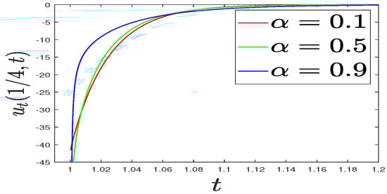
Let $\Omega =(0,1)$, $[a,T]=[1,1.2]$, $\kappa \left(t\right)=1$, $u_a\left(x\right)=sin\left(2\pi x\right)$ and $f(x,t)=0$, and select the numerical solution $\widehat{u}$ with $N=2^{10}$ and $h=1/32$ to be a reference solution. We plot the first-order time difference quotient ${\delta }_{t_n}{u}_{h,n}(1/4,t_n)$ in Figure 1. It is clear that the temporal derivative of the solution exhibits a singular behavior near the initial time, which gets stronger as α increases. These findings numerically satisfy Theorem 2.

Figure 1. Plots of ${\delta }_{t_n}{u}_{h,n}(\frac{1}{4},t_n)$: $\alpha =0.1,0.5,0.9$.

Example 2.

Let $={(0,1)}^2$, $[a,T]=[1,2]$, $u_a\left(x\right)=0$ and $\kappa \left(t\right)=1$. The exact solution to problem (1) is chosen to be $u={(logt)}^{2-\alpha }sin\left(2\pi x\right)sin\left(2\pi y\right)$ and f is calculated accordingly. We measure the convergence rates κ (temporal rate) and γ (spatial rate) by

$$\underset{1\le n\le N}{max}{\parallel u_n-u_{h,n}\parallel }_{L^2(\Omega )}\le Q(N^{-r_t}+M^{-r_s}).$$

The numerical results listed in Table 1 and Table 2 show that the finite element method retains a first-order accuracy in time and a second-order accuracy in space as proved in Theorem 5.

Table 1. Temporal convergence orders under different $\alpha$.

	$\alpha =\mathbf{0}.\mathbf{1}$		$\alpha =\mathbf{0}.\mathbf{5}$		$\alpha =\mathbf{0}.\mathbf{9}$
$N$	$M={\mathbf{2}}^{\mathbf{10}}$	$r_t$	$M={\mathbf{2}}^{\mathbf{10}}$	$r_t$	$M={\mathbf{2}}^{\mathbf{10}}$	$r_t$
32	4.61 $\times {10}^{-5}$		2.12 $\times {10}^{-5}$		8.64 $\times {10}^{-5}$
64	2.27 $\times {10}^{-5}$	1.02	1.11 $\times {10}^{-5}$	0.94	4.19 $\times {10}^{-5}$	1.04
128	1.13 $\times {10}^{-5}$	1.01	5.79 $\times {10}^{-6}$	0.94	2.07 $\times {10}^{-5}$	1.02
256	5.64 $\times {10}^{-6}$	1.00	2.97 $\times {10}^{-6}$	0.97	1.03 $\times {10}^{-5}$	1.01

Table 2. Spatial convergence orders under different $\alpha$.

	$\alpha =\mathbf{0}.\mathbf{1}$		$\alpha =\mathbf{0}.\mathbf{5}$		$\alpha =\mathbf{0}.\mathbf{9}$
$M$	$N={\mathbf{2}}^{\mathbf{12}}$	$r_s$	$N={\mathbf{2}}^{\mathbf{12}}$	$r_s$	$N={\mathbf{2}}^{\mathbf{12}}$	$r_s$
8	7.54 $\times {10}^{-4}$		1.55 $\times {10}^{-3}$		2.00 $\times {10}^{-3}$
16	1.93 $\times {10}^{-4}$	1.97	2.69 $\times {10}^{-4}$	1.97	5.11 $\times {10}^{-4}$	1.97
32	4.85 $\times {10}^{-5}$	1.99	6.77 $\times {10}^{-5}$	1.99	1.28 $\times {10}^{-4}$	2.00
64	1.22 $\times {10}^{-5}$	2.00	1.69 $\times {10}^{-5}$	2.00	3.10 $\times {10}^{-5}$	2.04

4. An Inversion Algorithm to Evaluate the Fractional Order $\alpha$

In many practical scenario problems, the fractional order $\alpha$ in model problem (1) is not clear. Therefore, we must use physical experiments to obtain the data.

4.1. L–M Regularization Method

We discuss an algorithm to simulate the fractional order $\alpha$ with the help of the finite element method (8) as follows: given the observation data ${\left\{{\theta }_i\right\}}_{i=1}^N$, the goal of the parameter identification of $\alpha$ is to find ${\alpha }_{inv}$ satisfying

$${\alpha }_{inv}=arg\underset{\alpha \in (0,1)}{min}\mathcal{F}\left(\alpha \right):=\frac{1}{2}\sum _{i=1}^N{\left(u(x_i,T;\alpha )-{\theta }_i\right)}^2.$$

(11)

In order to solve minimization problem (11), one can use an iterative algorithm such as Newton’s method. We used the first and second derivatives of the function $\mathcal{F}\left(\alpha \right)$ for minimizing (11)

$${\alpha }_{k+1}={\alpha }_k-\frac{{\mathcal{F}}^{{}^{\prime }}\left({\alpha }_k\right)}{{\mathcal{F}}^{{}^{\prime \prime }}\left({\alpha }_k\right)},$$

(12)

Here, k represents the kth iteration. Actually, relation (12) is equivalent to solving

$${\alpha }_{k+1}={\alpha }_k-{\left({\mathrm{J}}_k^{\top }{\mathrm{J}}_k\right)}^{-1}{\mathrm{J}}_k^{\top }{\mathrm{r}}_k,$$

(13)

where $r_k={(r_1,r_2,\cdots ,r_N)}^{\top }$ and $r_i=u(x_i,T;\alpha )-{\theta }_i$

$${\mathrm{J}}_k={\left(\frac{\partial u\left(x_1,T;\alpha \right)}{\partial \alpha },\cdots ,\frac{\partial u\left(x_N,T;\alpha \right)}{\partial \alpha }\right)}^{\top }\in {\mathbb{R}}^N.$$

(14)

We note that, in order to calculate the derivative $\frac{\partial u\left(x_i,T;\alpha \right)}{\partial \alpha }$, we can use the finite difference approximation

$$\frac{u(x_i,T;\alpha +\delta )-u(x_i,T;\alpha )}{\delta }$$

with a small $\delta$ to approximate the derivatives. However, the Newton method may sometimes fail to work due to ${\mathrm{J}}_k^{\top }{\mathrm{J}}_k\approx 0$. Usually, for dealing with this problem, we can apply the Levenberg–Marquardt algorithm to minimize (11) by

$${\alpha }_{k+1}={\alpha }_k-{\left({\mathrm{J}}_k^{\top }{\mathrm{J}}_k+{\gamma }_k\right)}^{-1}{\mathrm{J}}_k^{\top }{\mathrm{r}}_k,$$

(15)

where ${\gamma }_k$ is a positive penalty parameter. Thus, we give the program in Algorithm 1.

Algorithm 1:(A Levenberg–Marquardt Algorithm): Given the initial data, the boundary information and the observation data $\theta$.

1: For an initial guess ${\alpha }_0$ and $\rho \in (0,1)$, $\sigma \in (0,\frac{1}{2})$, ${\gamma }_0>0$ and a $\delta \ll 1$ . 2: for$k=1,\cdots , \mathit{Iterations}$ do 3:    Solve model problem (1) corresponding to ${\alpha }_k$ and ${\alpha }_k+\delta$, respectively, to get $u_r(·,T;{\alpha }_k)$ and $u_r(·,T;{\alpha }_k+\delta )$. 4:    Use formula (14) to calculate Jacobian ${\mathrm{J}}_k$ and ${\mathrm{J}}_k^{\top }{\mathrm{r}}_k$ and update the search direction $d_k:=-{\left({\mathrm{J}}_k^{\top }{\mathrm{J}}_k+{\gamma }_k\right)}^{-1}{\mathrm{J}}_k^{\top }{r}_k$. 5:    Identify the search step ${\rho }^m$ by the following Armijo rule: $$\mathcal{F}\left({\alpha }_k+{\rho }^m{d}_k\right)\le \mathcal{F}\left({\alpha }_k\right)+\sigma {\rho }^m{d}_k{\mathrm{J}}_k^{\top }{\mathrm{r}}_k.$$ 6:    If $\left|{\rho }^m{d}_k\right|\le \mathit{tolerance}$, then stop and let ${\alpha }_{inv}:={\alpha }_k$. Otherwise update ${\alpha }_{k+1}:={\alpha }_k+{\rho }^m{d}_k,{\gamma }_{k+1}:={\gamma }_k/2$, and go to Step 3. 7: end for

4.2. Numerical Experiment of the Finite Element Levenberg–Marquardt Method

Next, we ran some numerical examples to test the utility of the inverse method in model problem (1). Let ${\alpha }^{*}$ be the true order of model (1). Let ${\alpha }_0$ be an initial guess for the optimization, ${\alpha }_{inv}$ be the approximation order and “Iter” be the number of iterations. We took the observation data $\theta$ to be the exact solution of the problem (1) at T with fractional order ${\alpha }^{*}$.

Test 1.

In this test, we considered the data for the uncontaminated case.

Let$\kappa \left(t\right)=1$, the exact solution can be chosen as

$$u(x,t)={(logt)}^{2-\alpha }sin\left(2\pi x\right),$$

and the right-hand side can be computed accordingly. In Algorithm 1, we set$\rho =0.75,$$\sigma =0.25,$$\delta ={10}^{-4}$and the tolerance as${10}^{-10}$. We chose$N=M=100$in the finite element method with different initial guesses${\alpha }_0\in (0,1)$in the LM algorithm. We present the output${\alpha }_{inv}$and approximation error$|{\alpha }_{inv}-{\alpha }^{*}|$and we also give the total number of iterations inTable 3.

Table 3. Numerical observation of different ${\alpha }^{*}=0.3,0.6,0.9$ with different initial guesses ${\alpha }_0=0.2,0.5,0.8$ in Test 1.

${\alpha }^{*}$	${\alpha }_0$	${\alpha }_{inv}$	$\left|{\alpha }^{*}-{\alpha }_{inv}\right|$	Iter.
	$0.2$	2.9997 $\times {10}^{-1}$	3.4048 $\times {10}^{-5}$	11
$0.3$	$0.5$	2.9997 $\times {10}^{-1}$	3.3971 $\times {10}^{-5}$	11
	$0.8$	2.9997 $\times {10}^{-1}$	3.3984 $\times {10}^{-5}$	12
	$0.2$	5.9995 $\times {10}^{-1}$	5.1359 $\times {10}^{-5}$	12
$0.6$	$0.5$	5.9995 $\times {10}^{-1}$	5.1364 $\times {10}^{-5}$	11
	$0.8$	5.9995 $\times {10}^{-1}$	5.1287 $\times {10}^{-5}$	11
$0.9$	$0.2$	8.9994 $\times {10}^{-1}$	5.8136 $\times {10}^{-5}$	12
	$0.5$	8.9994 $\times {10}^{-1}$	5.8134 $\times {10}^{-5}$	12
	$0.8$	8.9994 $\times {10}^{-1}$	5.8135 $\times {10}^{-5}$	11

In Figure 2, Figure 3 and Figure 4, we plotted the variation of the errors and the cost functions with the number of iterations. From the figures, we can see that the proposed finite element LM method achieved a desired approximation ${\alpha }^{*}$ for different initial guesses.

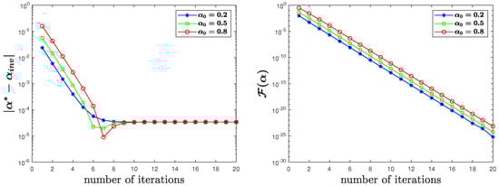
Figure 2. ${\alpha }^{*}=0.3$ for uncontaminated observation data in Test 1.

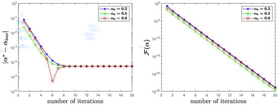
Figure 3. ${\alpha }^{*}=0.6$ for uncontaminated observation data in Test 1.

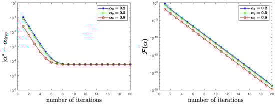
Figure 4. ${\alpha }^{*}=0.9$ for uncontaminated observation data in Test 1.

Test 2.

Because there may be noise in real problems, we tested cases in which the data were contaminated as follows:

$${\theta }^{ϵ}\left(x_i\right)=\theta \left(x_i\right)\left(1+ϵ\%·\mathit{randn}\left(\mathit{i}\right)\right),i=1,\cdots ,M.$$

(16)

where$ϵ$represents the degree of noise,$\mathit{randn}$denotes the random noise generated by the Gaussian distribution. The exact solution, initial condition and source term in this Test were the same as those in Test 1. We listed the numerical results in Table 4.

Table 4. Numerical results of different ${\alpha }^{*}=0.75$ with $ϵ\%$-degree noise-contaminated data in Test 2.

$ϵ\%$	${\alpha }_0$	${\alpha }_{\mathit{i}\mathit{n}\mathit{v}}$	$\left|{\alpha }^{*}-{\alpha }_{\mathit{i}\mathit{n}\mathit{v}}\right|$	Iter.
	$0.2$	7.4999 $\times {10}^{-1}$	1.1803 $\times {10}^{-5}$	12
$0.01$	$0.5$	7.4992 $\times {10}^{-1}$	7.6152 $\times {10}^{-5}$	12
	$0.8$	7.4967 $\times {10}^{-1}$	3.3354 $\times {10}^{-4}$	12
	$0.2$	7.5078 $\times {10}^{-1}$	7.8329 $\times {10}^{-4}$	12
$0.1$	$0.5$	7.5104 $\times {10}^{-1}$	1.0446 $\times {10}^{-3}$	12
	$0.8$	7.5257 $\times {10}^{-1}$	2.5709 $\times {10}^{-3}$	12
1	$0.2$	7.3639 $\times {10}^{-1}$	1.3607 $\times {10}^{-2}$	12
	$0.5$	7.4047 $\times {10}^{-1}$	9.5338 $\times {10}^{-3}$	12
	$0.8$	7.4961 $\times {10}^{-1}$	3.9271 $\times {10}^{-4}$	12

In Figure 5, Figure 6 and Figure 7, we also present the variation of errors and values of the cost function with iterations under different degrees of the noise. From the figures, we can see that our algorithm can obtain satisfactory results with a smaller number of iterations.

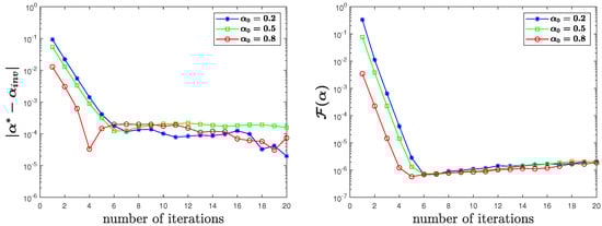
Figure 5. ${\alpha }^{*}=0.75$ for contaminated observation data with $0.01\%$ of noise in Test 2.

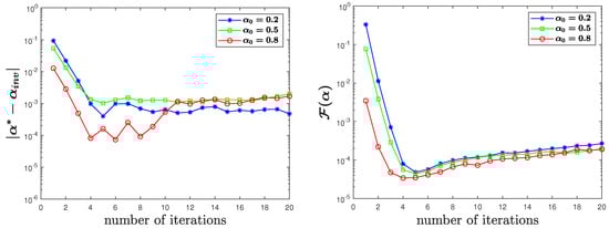
Figure 6. ${\alpha }^{*}=0.75$ for contaminated observation data with $0.1\%$ of noise in Test 2.

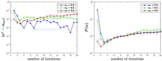
Figure 7. ${\alpha }^{*}=0.75$ for contaminated observation data with $1\%$ of noise in Test 2.

Test 3.

For the next test, we considered the two-dimensional case. Let$\kappa \left(t\right)=1$, the exact solution was chosen to be

$$u(x,y,t)={(logt)}^{2-\alpha }sin\left(2\pi x\right)sin\left(2\pi y\right),$$

and the right-hand side can be computed accordingly. The other data were the same as in Test 1. We chose$N=100$ and $h_x=h_y=1/100$ in the finite element method with different initial guesses ${\alpha }_0\in (0,1)$ in the LM algorithm. We present the numerical results in Table 5.

Table 5. Numerical results of different ${\alpha }^{*}=0.3,0.6,0.9$ with different initial guesses ${\alpha }_0=0.2,0.5,0.8$ in Test 3.

${\alpha }^{*}$	${\alpha }_0$	${\alpha }_{inv}$	$\left|{\alpha }^{*}-{\alpha }_{\mathit{i}\mathit{n}\mathit{v}}\right|$	Iter.
	$0.2$	3.008 $\times {10}^{-1}$	8.4911 $\times {10}^{-4}$	11
$0.3$	$0.5$	3.008 $\times {10}^{-1}$	8.4911 $\times {10}^{-4}$	11
	$0.8$	3.008 $\times {10}^{-1}$	8.4911 $\times {10}^{-4}$	12
	$0.2$	6.008 $\times {10}^{-1}$	8.3445 $\times {10}^{-4}$	12
$0.6$	$0.5$	6.008 $\times {10}^{-1}$	8.3445 $\times {10}^{-4}$	11
	$0.8$	6.008 $\times {10}^{-1}$	8.3445 $\times {10}^{-4}$	11
$0.9$	$0.2$	9.008 $\times {10}^{-1}$	8.3297 $\times {10}^{-4}$	12
	$0.5$	9.008 $\times {10}^{-1}$	8.3297 $\times {10}^{-4}$	12
	$0.8$	9.008 $\times {10}^{-1}$	8.3297 $\times {10}^{-4}$	11

We also plotted the change of parameter errors and values of the cost function with iterations in Figure 8, Figure 9 and Figure 10 and observed that the optimization process took only a few iterations to reach the tolerance.

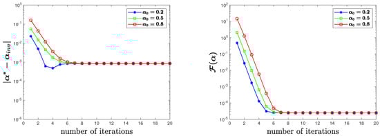
Figure 8. ${\alpha }^{*}=0.3$ for uncontaminated observation data in Test 3.

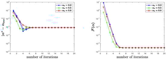
Figure 9. ${\alpha }^{*}=0.6$ for uncontaminated observation data in Test 3.

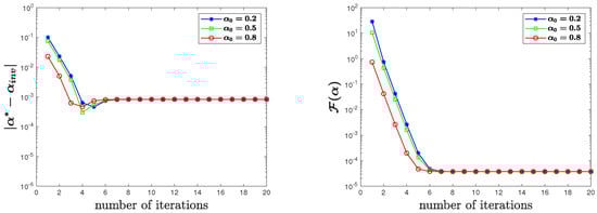
Figure 10. ${\alpha }^{*}=0.9$ for uncontaminated observation data in Test 3.

Test 4.

We also considered two-dimensional cases in which the data had a small random perturbation as follows:

$${\theta }^{ϵ}(x_i,y_j)=\theta (x_i,y_j)\left(1+ϵ\%·\mathit{randn}(\mathit{i},\mathit{j})\right),i,j=1,\cdots ,M.$$

(17)

The exact solution, initial condition and source term in this Test were the same as those in Test 3. The numerical results are listed inTable 6.

Table 6. Numerical observation of different ${\alpha }^{*}=0.75$ with data contaminated with $ϵ\%$ of noise in Test 4.

$ϵ\%$	${\alpha }_0$	${\alpha }_{inv}$	$\left|{\alpha }^{*}-{\alpha }_{\mathit{i}\mathit{n}\mathit{v}}\right|$	Iter.
	$0.2$	7.5085 $\times {10}^{-1}$	8.5595 $\times {10}^{-4}$	12
$0.01$	$0.5$	7.5082 $\times {10}^{-1}$	8.2265 $\times {10}^{-4}$	12
	$0.8$	7.5081 $\times {10}^{-1}$	8.1000 $\times {10}^{-4}$	12
	$0.2$	7.5089 $\times {10}^{-1}$	8.9797 $\times {10}^{-4}$	12
$0.1$	$0.5$	7.5076 $\times {10}^{-1}$	7.6190 $\times {10}^{-4}$	12
	$0.8$	7.5102 $\times {10}^{-1}$	1.0166 $\times {10}^{-3}$	12
1	$0.2$	7.5415 $\times {10}^{-1}$	4.1538 $\times {10}^{-3}$	12
	$0.5$	7.4991 $\times {10}^{-1}$	8.5762 $\times {10}^{-5}$	12
	$0.8$	7.5305 $\times {10}^{-1}$	3.0522 $\times {10}^{-3}$	12

From Figure 11, Figure 12 and Figure 13, we can see that when the observation data g are contaminated by random noise, the algorithm can still output satisfactory results in the two-dimensional case.

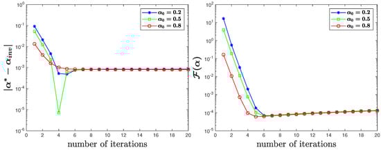
Figure 11. ${\alpha }^{*}=0.75$ for true data with $0.01\%$ of noise in Test 4.

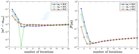
Figure 12. ${\alpha }^{*}=0.75$ for true data with $0.1\%$ of noise in Test 4.

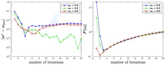
Figure 13. ${\alpha }^{*}=0.75$ for true data with $1\%$ of noise in Test 4.

5. Conclusions

We developed a finite element scheme for the numerical solution of two-timescale fractional diffusion Equation (1) involving a so-called Hadamard time-fractional derivative. We also proved the optimal convergence order of the error estimates of the finite element scheme to (1) without smooth assumptions on the true solution. Then, we presented several numerical examples to substantiate the mathematical and numerical analyses. We accordingly developed a finite element Levenberg–Marquardt algorithm to simulate the fractional order. In the near future, we will consider the variable-order case of the model problem (1).

References

- Atangana, A. On the stability and convergence of the time-fractional variable order telegraph equation. J. Comput. Phys. 2015, 293, 104–114. [Google Scholar] [CrossRef]
- Bai, X.; Rui, H. A second-order space-time accurate scheme for Maxwell’s equations in a Cole–Cole dispersive medium. Eng. Comput. 2022, 1, 1–20. [Google Scholar] [CrossRef]
- Bai, X.; Huang, J.; Rui, H.; Wang, S. Numerical simulation for 2D/3D time fractional Maxwell’s system based on a fast second-order FDTD algorithm. J. Comput. Appl. Math. 2022, 416, 114590. [Google Scholar] [CrossRef]
- Ma, J.; Gao, F.; Du, N. Stabilizer-free weak Galerkin finite element method with second-order accuracy in time for the time fractional diffusion equation. J. Comput. Appl. Math. 2022, 414, 114407. [Google Scholar] [CrossRef]
- Gu, X.; Sun, H.; Zhao, Y.; Zheng, X. An implicit difference scheme for time-fractional diffusion equations with a time-invariant type variable order. Appl. Math. Lett. 2021, 120, 107270. [Google Scholar] [CrossRef]
- Gu, X.; Wu, S. A parallel-in-time iterative algorithm for Volterra partial integro-differential problems with weakly singular kernel. J. Comput. Phys. 2020, 417, 109576. [Google Scholar] [CrossRef]
- Jia, J.; Wang, H. A preconditioned fast finite volume scheme for a fractional differential equation discretized on a locally refined composite mesh. J. Comput. Phys. 2015, 299, 842–862. [Google Scholar] [CrossRef]
- Jia, J.; Wang, H. A fast finite volume method on locally refined meshes for fractional diffusion equations. East Asian J. Appl. Math. 2019, 9, 755–779. [Google Scholar]
- Liu, Z.; Li, X.; Zhang, X. A fast high-order compact difference method for the fractal mobile/immobile transport equation. Int. J. Comput. Math. 2020, 97, 1860–1883. [Google Scholar] [CrossRef]
- Luchko, Y. Initial-boundary-value problems for the one-dimensional time-fractional diffusion equation. Fract. Calc. Appl. Anal. 2012, 15, 141–160. [Google Scholar] [CrossRef]
- Metzler, R.; Klafter, J. The random walk’s guide to anomalous diffusion: A fractional dynamics approach. Phys. Rep. 2000, 339, 1–77. [Google Scholar] [CrossRef]
- Schumer, R.; Benson, D.A.; Meerschaert, M.M.; Baeumer, B. Fractal mobile/immobile solute transport. Water Resour. Res. 2003, 39, 1–12. [Google Scholar] [CrossRef]
- Zheng, X.; Wang, H. An error estimate of a numerical approximation to a hidden-Memory variable-order space-time fractional diffusion equation. SIAM J. Numer. Anal. 2020, 58, 2492–2514. [Google Scholar] [CrossRef]
- Zheng, X.; Wang, H. A hidden-memory variable-order fractional optimal control model: Analysis and approximation. SIAM J. Control Optim. 2021, 59, 1851–1880. [Google Scholar] [CrossRef]
- Zheng, X. Logarithmic transformation between (variable-order) Caputo and Caputo-Hadamard fractional problems and applications. Appl. Math. Lett. 2021, 121, 107366. [Google Scholar] [CrossRef]
- Zheng, X.; Wang, H. Optimal-order error estimates of finite element approximations to variable-order time-fractional diffusion equations without regularity assumptions of the true solutions. IMA J. Numer. Anal. 2021, 41, 1522–1545. [Google Scholar] [CrossRef]
- Yang, Z.; Zheng, X.; Wang, H. A variably distributed-order time-fractional diffusion equation: Analysis and approximation. Comput. Methods Appl. Mech. Eng. 2020, 367, 113118. [Google Scholar] [CrossRef]
- Kilbas, A.A.; Srivastava, H.M.; Trujillo, J.J. Theory and Applications of Fractional Differential Equations; Elsevier: Amsterdam, The Netherlands, 2006; Volume 204. [Google Scholar]
- Ma, L.; Li, C. On Hadamard fractional calculus. Fractals 2017, 25, 1750033. [Google Scholar] [CrossRef]
- Hadamard, J. Essai sur l’étude des fonctions, données par leure développement de Taylor. J. Pure Appl. Math. 1892, 4, 101–186. [Google Scholar]
- Denisov, S.I.; Kantz, H. Continuous-time random walk theory of superslow diffusion. Europhys. Lett. 2010, 92, 30001. [Google Scholar] [CrossRef]
- Dräger, J.; Klafter, J. Strong anomaly in diffusion generated by iterated maps. Phys. Rev. Lett. 2000, 84, 5998. [Google Scholar] [CrossRef] [PubMed]
- Yang, Z.; Zheng, X.; Wang, H. Well-posedness and regularity of Caputo—Hadamard fractional stochastic differential equations. Z. Angew. Math. Phys. 2021, 72, 141. [Google Scholar] [CrossRef]
- Adams, R.A.; Fournier, J.J.F. Sobolev Spaces; Elsevier: San Diego, CA, USA, 2003. [Google Scholar]
- Bennett, C.; Sharpley, R.C. Interpolation of Operators; Academic Press: Orlando, FL, USA, 1988. [Google Scholar]
- Evans, L.C. Partial Differential Equations; Graduate Studies in Mathematics, V 19; American Mathematical Society: Providence, RI, USA, 1998. [Google Scholar]
- Servadei, R.; Valdinoci, E. On the spectrum of two different fractional operators. Proc. R. Soc. Edinb. Sect. A. 2014, 144, 831–855. [Google Scholar] [CrossRef]
- Sakamoto, K.; Yamamoto, M. Initial value/boundary value problems for fractional diffusion-wave equations and applications to some inverse problems. J. Math. Anal. Appl. 2011, 382, 426–447. [Google Scholar] [CrossRef]
- Yang, Z.; Zheng, X.; Wang, H. Well-posedness and regularity of Caputo-Hadamard time-fractional diffusion equations. Fractals 2022, 30, 2250005. [Google Scholar] [CrossRef]
- Li, C.; Li, Z.; Wang, Z. Mathematical analysis and the local discontinuous Galerkin method for Caputo—Hadamard fractional partial differential equation. J. Sci. Comput. 2020, 85, 1–27. [Google Scholar] [CrossRef]
- Wheeler, M.F. A priori L2 error estimates for Galerkin approximations to parabolic partial differential equations. SIAM Numer Anal. 1973, 10, 723–759. [Google Scholar] [CrossRef]
Publisher’s Note: MDPI stays neutral with regard to jurisdictional claims in published maps and institutional affiliations. |
© 2022 by the authors. Licensee MDPI, Basel, Switzerland. This article is an open access article distributed under the terms and conditions of the Creative Commons Attribution (CC BY) license (https://creativecommons.org/licenses/by/4.0/).