Sampled-Data Based Fault-Tolerant Control Design for Uncertain CE151 Helicopter System with Random Delays: Takagi-Sugeno Fuzzy Approach

Abstract

This study inspects the issue of robust reliable sampled data control (SDC) for a class of Takagi-Sugeno (TS) fuzzy CE151 Helicopter systems with time-varying delays and linear fractional uncertainties. Specifically, both the variation range and the distribution probability of the time delay are considered in the control input. The essential aspect of the suggested results in this study is that the time variable delay in the control input is dependent not only on the bound but also on the distribution probability of the time delay. The prime intent of this study is to enhance a state feedback reliable sampled-data controller. By constructing an appropriate Lyapunov-Krasovskii functional (LKF) and employing a linear matrix inequalities (LMIs) approach, a new set of delay-dependent necessary conditions is obtained to ensure the asymptotic stabilisation of a TS fuzzy CE151 Helicopter system with a prescribed mixed H_∞ and passivity (MH_∞P) performance index. The acquired results are expressed as LMIs, which are easily addressed using standard optimization algorithms. In addition, an exemplary scenario based on the CE151 helicopter model is presented to demonstrate the less conservative nature of the obtained results as well as the application of the recommended unique design approaches.

1. Introduction

In recent years, the fuzzy systems technique has become a famous and effective tool for analyzing and synthesising complex nonlinear systems. Among the numerous fuzzy modelling strategies, the Takagi-Sugeno (TS) fuzzy system [1,2,3], in which a linear system is used as the consequent component of a fuzzy rule, has piqued the interest of control theory and provides a simple and effective solution to dealing with complicated nonlinear control systems. Li et al. [3] investigated the topic of constructing fuzzy observer-based controllers for nonlinear networked control systems With a limited number of communication channels and parameter uncertainty. Tsai [4] demonstrated asymptotic stability for a category of TS fuzzy uncertain neutral systems using homogeneous polynomials and Polya’s theorem in terms of an LMI.

The assessment of the stability of TS fuzzy systems is one of the most critical topics. Many recent studies [5,6,7] have reported a great number of results for the Lyapunov stability analysis with various forms of control of TS fuzzy system utilising the LMI approach. Zhang et al. [7] used the LKF to offer innovative stability and stabilisation requirements for T-S fuzzy systems with less conservative LMI conditions. Yang et al. [8] use a delay-partitioning technique in conjunction with the free matrix based integral inequality to enhance the stability requirements of T-S fuzzy uncertain systems along with interval time delay.

Besides that, the SDC is a useful and practical technique for implementing numerous complicated control systems, and it has been applied in a wide range of scientific and technical disciplines [9]. Following then, the analysis of SDC systems that may have been characterized by TS fuzzy models has been extensively documented from across literature, for example, see [10]. Jiang [11] investigates the SDC of fuzzy control design strategy for TS design fuzzy systems with parameter uncertainties and LMI. Using the input delay approach, Liu and Zhou [12] proposed a problem of finite-time SDC for switching T-S fuzzy systems. Ge and Han [10] examined distributed asynchronous sampled-data H∞ filtering across a sensor network for a Markovian jump system.

It should be highlighted, however, that the time delay phenomenon occurs often in several practical systems and is widely recognized as a cause of instability [9,13,14]. More specifically, in dynamical systems, time delay oftenly appears to exist in a random pattern, implying that even some values of the time varying delay are indeed extremely large, but the probability of the delay attempting to capture such values is indeed very tiny, and considering the time delay’s range varying data can only lead to less conservative results [11,15]. Statistical approaches, for instance the Bernoulli and Poisson distributions, may also be used to derive their probabilistic properties. As a result, the random delay impact must be considered while studying time-varying dynamical system models [5,9]. Sakthivel et al. [5] explored dependable robust stabilisation for a category of TS fuzzy uncertain systems having time-delays, where the delay component is considered to be randomized and parameter uncertainties are accounted for using a linear fractional transformation form.

In addition, failures of control components such as sensors and actuators are common in realistic dynamical systems [2,16]. However, when a failure occurs, the traditional controller becomes conservative and may fail to meet certain control performance indices [15]. On the other hand, the reliable control maintains an acceptable stability performance for the closed-loop systems in the case of actuator or sensor failures [16,17]. Wei et al. [18] recently developed the resilient and reliable H_∞ static output control for nonlinear TS fuzzy discrete-time affine systems with actuator faults and parameter uncertainties, using the Markov chain to characterise the actuator-fault behaviours. Du et al. [15] addressed the issue of H_∞ reliable control for uncertain neural networks with varied time delays. Hu et al. [17] analyze the mode-dependent average dwell-time solution to the dependable guaranteed-cost control issue for a category of switched linear delta operator systems.

As previously noted, uncertainty is a source of performance loss in TS fuzzy systems. Because of modelling errors and changing environments, the description of fuzzy systems necessarily includes uncertainties, which may impact the performance and stability of fuzzy systems. A specific category of uncertainty in linear fractional transformation (LFT) has been established to cope with uncertainty in system dynamics, since it may contain norm-bounded uncertainties, as an example [5,19,20]. Sakthivel et al. [5] recently proposed the problem of resilient H_∞ reliable performance for fuzzy systems with LFT and random delays. Feng and Lam [19] devised the integral partitioning strategy to robust stabilisation utilising a distributed time delay system for LFT uncertain distributed time delay systems. To the extent of the researcher’s knowledge, no study on the sampled data reliable stabilization problem for a class of robust TS fuzzy CE150 Helicopter systems with random delays, LFT uncertainties and a mixed H_∞ and passivity approach has been discussed in the current literature.

The key advantage of this study is the establishment of a state feedback robust reliable SDC for a class of TS fuzzy CE150 helicopter systems with a MH_∞P performance level $\gamma >0$ as a consequence of the foregoing discussion. We acquire a novel set of necessary conditions for the delay-dependent robust H∞ reliable SDC design using the LKF in conjunction with the LMI approach, which makes sure the robust asymptotic stability of the regarded TS fuzzy system and also outcomes in the delay-dependent robust H_∞ reliable SDC design with random delay. The findings may also be be used to the robust stabilization of uncertain random delayed TS fuzzy CE151 Helicopter systems with LFT using a known and unknown reliable sampled robust control. The following are the features of this paper’s contribution.

*

A novel reliable SDC state feedback control strategy is considered for the uncertain TS fuzzy CE151 Helicopter systems with time-varying delays.

*

The effects of variation range and probability distribution of time-delays are also explored in the proposed study. Additionally, the uncertainties in the system are assumed to be in the form of LFT.

*

The main objective of this paper is to design a reliable SDC controller such that the resulting closed loop form of the system is robustly asymptotically stable with a desired MH_∞P disturbance attenuation level $\gamma >0.$

*

A robust reliable SDC MH_∞P controller is designed for attaining the needed result based on a proper Lyapunov-Krasovskii functional and LMI approach. The resultant results are expressed in terms of LMI, which is easily computed to use the MATLAB-LMI toolbox.

Finally, a numerical example based on the CE151 Helicopter model is used to demonstrate the efficacy and utility of the suggested technique.

2. System Description and Problem Formulation

In this work, we will look at the CE151 helicopter model, which is available from Humusoft Ltd. The system is made up of a body that houses two propellers powered by direct current motors and a huge support. The human body has two degrees of freedom. The body’s position angles (both horizontal and vertical) are adjusted according to the rotation of the propellers. A body’s axes of rotation are perpendicular to one another. Both points of view are taken into account. A servomotor moves a small weight along the helicopter’s primary horizontal axis, adjusting the helicopter’s centre of gravity. As shown in the picture, the mathematical model of the whole helicopter system is a conventional MIMO $2\times 2$ system with significant cross couplings. In this situation, the horizontal body position angle is fixed, and the helicopter is only examined in vertical position [6] for the sake of this research. Figure 1 depicts a silhouette of the CE151 helicopter model.

The helicopter’s dynamics in elevation may be described, as follows, using the following equation:

$$\begin{array}{ccc}\hfill I\ddot{\psi }& =& \tau -{\tau }_f-{\tau }_m\hfill \end{array}$$

(1)

where I is the helicopter body’s rotating moment of inertia around its horizontal axis, $\tau$ denotes the elevation driving torque, ${\tau }_f$ represents the friction torque, ${\tau }_m$ is the gravity torque and $\psi$ is the angle of elevation. The elevation driving torque is controlled by the delay in the motor-propeller process. $\psi =0$ indicates that the helicopter’s body is oriented downward, while $\psi =\frac{\pi }{2}\left({90}^{\circ }\right)$ indicates that the helicopter’s body is positioned horizontally. The initial condition of the body’s resting potential is $\psi =\frac{\pi }{4}\left({45}^{\circ }\right).$ The following are real relationships:

$$\begin{array}{ccc}\hfill {\tau }_f& =& B_{\psi }\dot{\psi }\hfill \end{array}$$

(2)

$$\begin{array}{ccc}\hfill {\tau }_m& =& mglsin\psi \stackrel{\Delta }{=}{\tau }_{g}sin\psi \hfill \end{array}$$

(3)

where $B_{\psi }$ symbolises the friction constant, m the helicopter’s mass, g the gravitational constant and l the distance between the helicopter’s body’s centre of gravity and the supported point. The dynamics of the motor-propeller are supposed to obey a set of laws.

$$\begin{array}{ccc}\hfill \tau & =& a{u}_d^2+b{u}_d\hfill \\ \hfill T^2{\ddot{u}}_d+2T{\dot{u}}_d+u_d& =& u\hfill \end{array}$$

(4)

where $u_d$ is the armature voltage u denotes the control input and $a,b$ and T are some constant scalars. All the constant scalars are identified as follows; $I=2.64\times {10}^{-3},B_{\psi }=5.43\times {10}^{-3},$${\tau }_g=7.66\times {10}^{-2},a=0.109,b=2.76\times {10}^{-2},T=0.2$. However, these parameters may have some identification errors. Now, define a new state vector $x\left(t\right)=\left[\begin{array}{cccc}\psi & u_d& \dot{\psi }& {\dot{u}}_d\end{array}\right]$ and by introducing an input disturbance signal $w\left(t\right)$, LFT and reliable control with output $z\left(t\right)$ signal into account, then the uncertain TS fuzzy helicopter system (1) could be highlighted as,

Plant Ruleη:

IF $\left\{{\theta }_1\left(t\right)\mathrm{is}{M}_1^{\eta }\right\}$, $\left\{{\theta }_2\left(t\right)\mathrm{is}{M}_2^{\eta }\right\}$,…, $\left\{{\theta }_p\left(t\right)\mathrm{is}{M}_p^{\eta }\right\}$THEN

$$\begin{array}{c}\hfill \begin{array}{ccc}\dot{x}\left(t\right)\hfill & =\hfill & (A_{\eta }+H_{\eta }{\Delta }_{\eta }\left(t\right)E_{1\eta })x\left(t\right)+B_{\eta }{u}^f\left(t\right)+C_{\eta }w\left(t\right)\hfill \\ z\left(t\right)\hfill & =\hfill & D_{\eta }x\left(t\right)\hfill \end{array}\end{array}$$

(5)

where,

$$\begin{array}{ccc}\hfill A_{\eta }& =& \left[\begin{array}{cccc}0& 0& 1& 0\\ 0& 0& 0& 1\\ -\frac{{\tau }_{g}cos{\overline{\psi }}_{\eta }}{I}& \frac{2a{\overline{u}}_{d\eta }+b}{I}& -\frac{B_{\psi }}{I}& 0\\ 0& -\frac{1}{T^2}& 0& -\frac{2}{T}\end{array}\right],B_{\eta }={\left[\begin{array}{cccc}0& 0& 0& \frac{1}{T^2}\end{array}\right]}^T,C_{\eta }=I,\hfill \end{array}$$

where, $M_j^{\eta },(j=1,2,\dots ,p,\eta =1,2,\dots ,r)$ are fuzzy sets, ${\left\{{\theta }_1\left(t\right),{\theta }_2\left(t\right),\dots ,{\theta }_p\left(t\right)\right\}}^T$ are the vectors of the premise variables; r represents the quantity of IF-THEN rules; $D_{\eta },E_{\eta },H_{\eta }$ and $E_{1\eta }$ are known constant matrices of suitable dimensions.

The linear fractional form, which may incorporate the norm bounded uncertainty as a special instance, is described and demonstrated to be effective in [21]. Admissibility is defined as the set of uncertainty parameters ${\Delta }_{\eta }\left(t\right)$ that fulfill the constraint ${\Delta }_{\eta }\left(t\right)={\left[I-F_{\eta }\left(t\right)J\right]}^{-1}{F}_{\eta }\left(t\right),$ where J is also a recognized matrix fulfilling $I-J{J}^T>0$ and $F\left(t\right)$ is a time-varying undetermined matrix with Lebesgue measurable elements limited by $F_{\eta }^T\left(t\right)F_{\eta }\left(t\right)\le I$ ([19,21,22]).

The normalised membership function of the inferred fuzzy set ${\beta }_{\eta }\left(\xi \left(t\right)\right)$ is denoted by the notation ${\lambda }_{\eta }\left(\xi \left(t\right)\right)$ in this example. An assumption regarding the defuzzified helicopter system is as demonstrated below:

$$\begin{array}{c}\hfill \begin{array}{c}\dot{x}\left(t\right)={\displaystyle \sum _{\eta =1}^r}{\lambda }_{\eta }\left(\xi \left(t\right)\right)\left\{(A_{\eta }+H_{\eta }{\Delta }_{\eta }\left(t\right)E_{1\eta })x\left(t\right)+B_{\eta }{u}^f\left(t\right)+C_{\eta }w\left(t\right)\right\},\hfill \\ z\left(t\right)={\displaystyle \sum _{\eta =1}^r}{\lambda }_{\eta }\left(\xi \left(t\right)\right)\left\{D_{\eta }x\left(t\right)\right\},\hfill \end{array}\end{array}$$

(6)

where ${\lambda }_{\eta }\left(\xi \left(t\right)\right)=\frac{{\beta }_{\eta }\left(\xi \left(t\right)\right)}{{\displaystyle \sum _{\eta =1}^r}{\beta }_{\eta }\left(\xi \left(t\right)\right)}$ with ${\beta }_{\eta }\left(\xi \left(t\right)\right)={\displaystyle \prod _{i=1}^p}{M}_i^{\eta }\left({\xi }_i\left(t\right)\right)$ in which $M_i^{\eta }\left({\xi }_i\left(t\right)\right)$ is the grade of the membership function of ${\xi }_i\left(t\right)$ in $M_i^{\eta }$. Furthermore, we suppose ${\beta }_{\eta }\left(\xi \left(t\right)\right)\ge 0$, $\eta =1,2,\dots ,r$, ${\displaystyle \sum _{\eta =1}^r}{\beta }_{\eta }\left(\xi \left(t\right)\right)>0$, and ${\lambda }_{\eta }\left(\xi \left(t\right)\right)$ satisfy ${\lambda }_{\eta }\left(\xi \left(t\right)\right)\ge 0$, $\eta =1,2,\dots ,r$, ${\displaystyle \sum _{\eta =1}^r}{\lambda }_{\eta }\left(\xi \left(t\right)\right)=1$ for any $\xi \left(t\right)$.

The fundamental aim of this research is to create a control rule with the minimum possible $H_{\infty }$ performance index to ensure robust stability for the closed loop TS fuzzy helicopter system. To do this, we categorize actuator failures as follows:

$$\begin{array}{c}\hfill u^f\left(t\right)=G_{\eta }u\left(t\right),\end{array}$$

(7)

where $G_{\eta }$ is the actuator failure matrix, as defined in [5].

$$\begin{array}{c}\hfill G_{\eta }=\mathrm{d}\mathrm{i}\mathrm{a}\mathrm{g}\left\{g_{1\eta },g_{2\eta },\cdots ,g_{m\eta }\right\},0\le {\underline{g}}_{k\eta }\le g_{k\eta }\le {\overline{g}}_{k\eta }\le 1,\end{array}$$

(8)

where ${\underline{g}}_{k\eta }$ and ${\overline{g}}_{k\eta },\eta =1,2,\cdots ,r,k=1,2,\cdots ,m$ are provided with constants. In addition, we provide $G_{0\eta }=\mathrm{diag}\left\{g_{10\eta },g_{20\eta },\cdots ,g_{m0\eta }\right\}$, $g_{k0\eta }=\frac{{\overline{g}}_{k\eta }+{\underline{g}}_{k\eta }}{2}$, $G_{1\eta }=diag$$\left\{g_{11\eta },g_{21\eta },\cdots ,g_{m1\eta }\right\}$, $g_{k1\eta }=\frac{{\overline{g}}_{k\eta }-{\underline{g}}_{k\eta }}{2}$. Then the matrix $G_{\eta }$ can be written as

$$\begin{array}{ccc}\hfill G_{\eta }& =& G_{0\eta }+{\Delta }_{\eta }=G_{0\eta }+\mathrm{d}\mathrm{i}\mathrm{a}\mathrm{g}\left\{{\theta }_{1\eta },\cdots ,{\theta }_{m\eta }\right\},\hfill \\ \hfill \left|{\theta }_{k\eta }\right|& \le & g_{k1\eta },(k=1,\cdots ,m,\eta =1,\cdots ,r).\hfill \end{array}$$

(9)

 Remark 1. 

In (8), parameters ${\underline{g}}_{k\eta }$ and ${\overline{g}}_{k\eta }$ characterize the admissible failures of the signal from the controller. Obviously, when ${\underline{g}}_{k\eta }={\overline{g}}_{k\eta }=0$, denotes that the actuator completely fails (case of the outage). When $0\le {\underline{g}}_{k\eta }<{\overline{g}}_{k\eta }\le 1$, it corresponds to the case of partial failure. If ${\underline{g}}_{k\eta }={\overline{g}}_{k\eta }=1$, then the actuator is normal.

In this work, we examine the SDC input provided by a variable time delay as shown below.

$$\begin{array}{ccc}\hfill u\left(t\right)& =& u_d\left(t_k\right)=u_d(t-(t-t_k))=u_d(t-\tau \left(t\right)),t_k\le t\le t_{k+1},\tau \left(t\right)=t-t_k,\hfill \end{array}$$

(10)

where $u_d$ represent the discrete-time control signal, and the time varying delay $0\le \tau \left(t\right)=t-t_k$ is piecewise linear with the derivative $\dot{\tau }\left(t\right)=1,fort\ne t_k,$$t_k$ denote the sampling instant satisfying $0<t_1<t_2<\cdots <t_k<\cdots$. Specify the sampling interval $h_k=t_{k+1}-t_k,$ that can vary but is perpetually bounded. Afterwards, we have $\tau \left(t\right)\le t_{k+1}-t_k=h_k\le h$ for all $t_k$, where h represent the maximum upper bound of the sampling interval $h_k$.

In this study, we selected the SDC input in the approach

$$\begin{array}{ccc}\hfill u\left(t\right)& =& Kx\left(t_k\right).\hfill \end{array}$$

(11)

A piecewise control rule, as defined in (10), is a continuous time control with a time variable piecewise continuous delay $\tau \left(t\right)=t-t_k.$ As a response, we require the following state feedback controller design:

$$\begin{array}{ccc}\hfill u\left(t\right)& =& Kx(t-\tau (t\left)\right).\hfill \end{array}$$

(12)

This accompanying is the definition of the fuzzy control rule:

Control Rule η:

IF $\left\{{\theta }_1\left(t\right)\mathrm{is}{M}_1^{\eta }\right\}$, $\left\{{\theta }_2\left(t\right)\mathrm{is}{M}_2^{\eta }\right\}$,…, $\left\{{\theta }_p\left(t\right)\mathrm{is}{M}_p^{\eta }\right\}$ THEN

$$\begin{array}{c}\hfill u\left(t\right)=K_{\eta }x(t-\tau \left(t\right)),\end{array}$$

(13)

The following is a brief description of the entire fuzzy controller:

$$\begin{array}{c}\hfill u\left(t\right)={\displaystyle \sum _{\eta =1}^r}{\lambda }_{\eta }\left(\xi \left(t\right)\right)K_{\eta }x(t-\tau \left(t\right)),\end{array}$$

(14)

where $K_{\eta }(\eta =1,2,\cdots ,r)$ represents the control gains. When $u^f\left(t\right)$ is replaced for $u\left(t\right)$ in (6), and (14) and (7) are taken into consideration, the resultant closed-loop fuzzy systems are as described in the following:

$$\begin{array}{c}\hfill \begin{array}{ccc}\dot{x}\left(t\right)\hfill & =\hfill & {\displaystyle \sum _{\eta =1}^r}{\displaystyle \sum _{j=1}^r}{\lambda }_{\eta }\left(\xi \left(t\right)\right){\lambda }_j\left(\xi \left(t\right)\right)\left\{(A_{\eta }+H_{\eta }{\Delta }_{\eta }\left(t\right)E_{1\eta })x\left(t\right)+B_{\eta }{G}_{\eta }{K}_{\eta }x(t-\tau \left(t\right))+C_{\eta }w\left(t\right)\right\}.\hfill \end{array}\end{array}$$

(15)

Time delay was considered to be random in the systems that came before it, as well as satisfying the following assumptions:

 Assumption 1 

([5]). If $\tau \left(t\right)$ recognizes values in $[0:{\tau }_0]$ or $({\tau }_0:\overline{\tau }]$ and $Prob\{\tau \left(t\right)\in [0:{\tau }_0]\}={\delta }_0$ or $Prob\{\tau \left(t\right)\in ({\tau }_0:\overline{\tau }]\}=1-{\delta }_0,$ where ${\tau }_0$ and $\overline{\tau },$ then the time-varying delay $\tau \left(t\right)$ is restricted in such a manner that $0\le \tau \left(t\right)\le \overline{\tau }$ and its probability distribution can be observed, then the time-varying. It should be noted that, although some delay values are quite large in reality, the probabilities of such delays occuring are extremely minimal in practise. Given this, a scalar ${\tau }_0$ that fulfils the constraint $0\le {\tau }_0<\overline{\tau }$ is included in this section.

To describe a method for deriving the probability distribution of a time-varying delay, and the following set of functions is used to represent that probability distribution.

$$\begin{array}{c}\hfill {\mathcal{D}}_1=\left\{t|\tau \left(t\right)\in [0:{\tau }_0]\right\} \mathrm{a}\mathrm{n}\mathrm{d} {\mathcal{D}}_2=\left\{t|\tau \left(t\right)\in ({\tau }_0:\overline{\tau }]\right\}.\end{array}$$

(16)

In addition, we create two mapping functions, which are listed below:

$$\begin{array}{c}\hfill {\tau }_1\left(t\right)=\left\{\begin{array}{c}\tau \left(t\right),t\in {\mathcal{D}}_1\hfill \\ {\overline{\tau }}_1,t\in {\mathcal{D}}_2,\hfill \end{array}\right.\mathrm{a}\mathrm{n}\mathrm{d} {\tau }_2\left(t\right)=\left\{\begin{array}{c}\tau \left(t\right),t\in {\mathcal{D}}_2\hfill \\ {\overline{\tau }}_2,t\in {\mathcal{D}}_1.\hfill \end{array}\right.\end{array}$$

(17)

where ${\overline{\tau }}_1=[0:{\tau }_0]$ and ${\overline{\tau }}_2=({\tau }_0:\overline{\tau }]$.

 Assumption 2 

([5]). Furthermore, the time-varying delays ${\tau }_1\left(t\right)$ and ${\tau }_2\left(t\right)$ fulfilling the condition

$$\begin{array}{c}\hfill \begin{array}{c}0\le {\tau }_1\left(t\right)\le {\tau }_0,{\dot{\tau }}_1\left(t\right)=1,{\tau }_0<{\tau }_2\left(t\right)\le \overline{\tau },{\dot{\tau }}_2\left(t\right)=1.\hfill \end{array}\end{array}$$

(18)

The positive constants ${\tau }_0$ and $\overline{\tau }$ are both used in this equation. Further detail on the probability distribution delay issue can be found in the paper [5], which can be found here.

Further, as a result of (16) that ${\mathcal{D}}_1\cup {\mathcal{D}}_2={\mathbb{Z}}_{\ge 0},{\mathcal{D}}_1\cap {\mathcal{D}}_2=\Phi$, where $\Phi$ denote the empty set. It is simple to verify that $t\in {\mathcal{D}}_1$ implies the event $\tau \left(t\right)\in [0,{\tau }_0]$ occurs and $t\in {\mathcal{D}}_2$ implies the event $\tau \left(t\right)\in ({\tau }_0,\overline{\tau }]$ occurs.

Define a Bernoulli distributed stochastic variable

$$\begin{array}{c}\hfill \delta \left(t\right)=\left\{\begin{array}{c}1,t\in {\mathcal{D}}_1\hfill \\ 0,t\in {\mathcal{D}}_2.\hfill \end{array}\right.\end{array}$$

(19)

 Remark 2 

([5]). The variable $\delta \left(t\right)$ is Bernoulli distributed white sequences with $Prob\left\{\delta \right(t)=1\}=Prob\left\{\tau \right(t)\in [0$, ${\tau }_0\left]\right\}=\mathbb{E}\left[\delta \left(t\right)\right]={\delta }_0$ and $Prob\{\delta \left(t\right)=0\}=Prob\{\tau \left(t\right)\in ({\tau }_0$, $\overline{\tau }\left]\right\}=1-\mathbb{E}\left[\delta \left(t\right)\right]=1-{\delta }_0$. Moreover, it is easy to observe that $\mathbb{E}[\delta \left(t\right)-{\delta }_0]=0,\mathbb{E}\left[{(\delta \left(t\right)-{\delta }_0)}^2\right]={\delta }_0(1-{\delta }_0)$, where $0\le {\delta }_0\le 1$.

The TS fuzzy uncertain helicopter system (15) may be expressed in the following way by incorporating the random delay.

$$\begin{array}{c}\hfill \begin{array}{ccc}\dot{x}\left(t\right)\hfill & =\hfill & {\displaystyle \sum _{\eta =1}^r}{\displaystyle \sum _{j=1}^r}{\lambda }_{\eta }\left(\xi \left(t\right)\right){\lambda }_j\left(\xi \left(t\right)\right)\{(A_{\eta }+H_{\eta }{\Delta }_{\eta }\left(t\right)E_{1\eta })x\left(t\right)+\delta \left(t\right)B_{\eta }{G}_{\eta }{K}_{\eta }x(t-{\tau }_1\left(t\right))\hfill \\ & & +(1-\delta \left(t\right))B_{\eta }{G}_{\eta }{K}_{\eta }x(t-{\tau }_2\left(t\right))+C_{\eta }w\left(t\right)\}.\hfill \end{array}\end{array}$$

(20)

The definitions listed below are required to demonstrate our key findings.

 Definition 1 

([23]). If the system (20) is robustly asymptotically stable with a specific disturbance attenuation level $\gamma >0$ and the output $z\left(t\right)$ with zero initial condition fulfills, the system is robustly asymptotically stable

$$\begin{array}{c}\hfill {\int }_0^t(-{\gamma }^{-1}\beta z^T\left(s\right)z\left(s\right)+2(1-\beta )z^T\left(s\right)w\left(s\right))ds\ge -\gamma {\int }_0^t{w}^T\left(s\right)w\left(s\right)ds\end{array}$$

(21)

for all $t>0$ and any non-zero $w\left(t\right)\in L_2[0,\infty ]$, where $\beta \in [0,1]$ is perhaps a weighting parameter that specifies the trade-off between $H_{\infty }$ and passivity performances.

 Remark 3. 

Mixed H_∞ and passivity performance is a special case of dissipativity, which is first proposed in [24]. In Definition 1, β takes values on [0,1]. If β = 1, (21) reduces to the H_∞ performance; and if β = 0, (21) reduces to the passivity condition.

 Lemma 1 

([5]). Given adequate dimension matrices $\mathrm{\Pi }={\mathrm{\Pi }}^T$, S and N, the inequality

$$\begin{array}{c}\hfill \mathrm{\Pi }+S\Delta \left(t\right)N+N^T\Delta {\left(t\right)}^T{S}^T<0\end{array}$$

valid for $F\left(t\right)$ in such a way that $F^T\left(t\right)F\left(t\right)\le I$ if and only if some of $ϵ>0$,

$$\begin{array}{c}\hfill \left[\begin{array}{ccc}\mathrm{\Pi }& S& ϵN^T\\ S^T& -ϵI& ϵJ^T\\ ϵN& ϵJ& -ϵI\end{array}\right]<0.\end{array}$$

3. Main Results

We construct a state-feedback reliable SDC based on the LKF algorithm in this section, which ensures that the closed-loop TS fuzzy helicopter system with time-varying input random delay is asymptotically stable. We start by explaining the asymptotic stabilization of a TS fuzzy helicopter system without uncertainty using a reliable SDC with a MH_∞P performance attenuation level. As in the scenario, we utilize the TS fuzzy helicopter system in its nominal form, as follows;

$$\begin{array}{c}\hfill \begin{array}{ccc}\dot{x}\left(t\right)\hfill & =\hfill & {\displaystyle \sum _{\eta =1}^r}{\displaystyle \sum _{j=1}^r}{\lambda }_{\eta }\left(\xi \left(t\right)\right){\lambda }_j\left(\xi \left(t\right)\right)\{A_{\eta }x\left(t\right)+\delta \left(t\right)B_{\eta }{G}_{\eta }{K}_{\eta }x(t-{\tau }_1\left(t\right))\hfill \\ & & +(1-\delta \left(t\right))B_{\eta }{G}_{\eta }{K}_{\eta }x(t-{\tau }_2\left(t\right))+C_{\eta }w\left(t\right)\}.\hfill \end{array}\end{array}$$

(22)

Furthermore, this result is extended for the TS fuzzy uncertain helicopter system (20) with random input delay.

 Theorem 1. 

For given parameters ${\tau }_0,\overline{\tau },\beta ,\lambda$ and ${\delta }_0$ with known actuator failure matrix $G_{\eta }$, then the TS fuzzy helicopter system with random delay (22) is asymptotically stable with the MH_∞P performance $\gamma >0,$ if there exist symmetric matrices $X,{\tilde{Q}}_i,{\tilde{R}}_i,{\tilde{S}}_i,{\tilde{T}}_i,i=1,2,3$ and appropriate dimensioned matrices $Y_{\eta }$, such that the following LMIs applicable for $\eta ,j=1,2,\cdots ,r$;

$$\begin{array}{c}\hfill {\tilde{\mathrm{\Pi }}}_{\eta j}=\left[\begin{array}{cc}{\tilde{\mathrm{\Pi }}}_{(m,n)\eta j}& {\tilde{\mathrm{\Pi }}}_1^T\\ *& -\gamma \end{array}\right],m,n=1,2,\cdots ,12\end{array}$$

(23)

with

$$\begin{array}{ccc}\hfill {\mathrm{\Pi }}_{(1,1)\eta j}& =& {\tilde{Q}}_1+{\tilde{Q}}_2+{\tilde{Q}}_3+{\tau }_0{\tilde{R}}_1+(\overline{\tau }-{\tau }_0){\tilde{R}}_2+\overline{\tau }{\tilde{R}}_3-\frac{1}{{\tau }_0}{\tilde{S}}_1-\frac{1}{\overline{\tau }}{\tilde{S}}_3-2{\tilde{T}}_1-2\frac{\overline{\tau }-{\tau }_0}{\overline{\tau }+{\tau }_0}{\tilde{T}}_2-2{\tilde{T}}_3,\hfill \\ \hfill {\mathrm{\Pi }}_{(1,3)\eta j}& =& \frac{1}{{\tau }_0}{\tilde{S}}_1,{\mathrm{\Pi }}_{(1,4)\eta j}=\frac{1}{\overline{\tau }}{\tilde{S}}_3,{\mathrm{\Pi }}_{(1,6)\eta j}=2X+X{A}_{\eta }^T{\lambda }^T,{\mathrm{\Pi }}_{(1,7)\eta j}=\frac{2}{{\tau }_0}{\tilde{T}}_1,{\mathrm{\Pi }}_{(1,8)\eta j}=\frac{2}{{\tau }_0}{\tilde{T}}_1,\hfill \\ \hfill {\mathrm{\Pi }}_{(1,9)\eta j}& =& \frac{2}{(\overline{\tau }+{\tau }_0)}{\tilde{T}}_2+\frac{2}{\overline{\tau }}{\tilde{T}}_3,{\mathrm{\Pi }}_{(1,10)\eta j}=\frac{2}{(\overline{\tau }+{\tau }_0)}{\tilde{T}}_2,{\mathrm{\Pi }}_{(1,11)\eta j}=\frac{2}{\overline{\tau }}{\tilde{T}}_3,\hfill \\ \hfill {\mathrm{\Pi }}_{(1,12)\eta j}& =& -2(1-\beta )X{D}_{\eta }^T,{\mathrm{\Pi }}_{(2,2)\eta j}=-{\tilde{Q}}_1-{\tilde{Q}}_3-\frac{2}{{\tau }_0}{S}_1-\frac{2}{(\overline{\tau }-{\tau }_0)}{\tilde{S}}_2,{\mathrm{\Pi }}_{(2,3)\eta j}=\frac{1}{{\tau }_0}{\tilde{S}}_1,\hfill \\ \hfill {\mathrm{\Pi }}_{(2,4)\eta j}& =& \frac{1}{(\overline{\tau }-{\tau }_0)}{\tilde{S}}_2,{\mathrm{\Pi }}_{(2,6)\eta j}={\delta }_0{Y}_{\eta }^T{G}_{\eta }^T{B}_{\eta }^T\lambda ,{\mathrm{\Pi }}_{(3,3)\eta j}=-\frac{2}{{\tau }_0}{\tilde{S}}_1,{\mathrm{\Pi }}_{(3,6)\eta j}=(1-{\delta }_0)Y_{\eta }^T{G}_{\eta }^T{B}_{\eta }^T{\lambda }^T,\hfill \\ \hfill {\mathrm{\Pi }}_{(4,4)\eta j}& =& -\frac{2}{(\overline{\tau }-{\tau }_0)}({\tilde{S}}_2+{\tilde{S}}_3),{\mathrm{\Pi }}_{(4,5)\eta j}=\frac{2}{(\overline{\tau }-{\tau }_0)}({\tilde{S}}_2+{\tilde{S}}_3),{\mathrm{\Pi }}_{(5,5)\eta j}=-Q_2-\frac{1}{(\overline{\tau }-{\tau }_0)}({\tilde{S}}_2+{\tilde{S}}_3),\hfill \\ \hfill {\mathrm{\Pi }}_{(6,6)\eta j}& =& {\tau }_0{\tilde{S}}_1+(\overline{\tau }-{\tau }_0){\tilde{S}}_2+\overline{\tau }{\tilde{S}}_3-\lambda X,{\mathrm{\Pi }}_{(6,12)\eta j}=\lambda C_{\eta },{\mathrm{\Pi }}_{(7,7)\eta j}=-\frac{1}{{\tau }_0}{\tilde{R}}_1-\frac{2}{{\tau }_0^2}{\tilde{T}}_1,\hfill \\ \hfill {\mathrm{\Pi }}_{(7,8)\eta j}& =& -\frac{2}{{\tau }_0^2}{\tilde{T}}_1,{\mathrm{\Pi }}_{(8,8)\eta j}=-\frac{1}{{\tau }_0}{\tilde{R}}_1-\frac{2}{{\tau }_0^2}{\tilde{T}}_1,{\mathrm{\Pi }}_{(9,9)\eta j}=-\frac{1}{(\overline{\tau }-{\tau }_0)}({\tilde{R}}_2+{\tilde{R}}_3)-\frac{2}{({\overline{\tau }}^2-{\tau }_0^2)}{\tilde{T}}_2-\frac{2}{{\overline{\tau }}^2}{\tilde{T}}_3,\hfill \\ \hfill {\mathrm{\Pi }}_{(9,10)\eta j}& =& -\frac{2}{({\overline{\tau }}^2-{\tau }_0^2)}{\tilde{T}}_2,{\mathrm{\Pi }}_{(9,11)\eta j}=-\frac{1}{{\overline{\tau }}^2}{\tilde{T}}_3,{\mathrm{\Pi }}_{(10,10)\eta j}=-\frac{1}{(\overline{\tau }-{\tau }_0)}{\tilde{R}}_2-\frac{2}{({\overline{\tau }}^2-{\tau }_0^2)}{\tilde{T}}_2,\hfill \\ \hfill {\mathrm{\Pi }}_{(11,11)\eta j}& =& -\frac{1}{\overline{\tau }}{\tilde{R}}_3-\frac{2}{{\overline{\tau }}^2}{\tilde{T}}_3,{\mathrm{\Pi }}_{(12,12)\eta j}=-\gamma ,{\mathrm{\Pi }}_1=\left[\begin{array}{cc}\sqrt{\beta }X{D}_{\eta }& 0_{10n}\end{array}\right].\hfill \end{array}$$

All of the other parameters are set to zero. When applied to this situation, $K_{\eta }=Y_{\eta }{X}^{-1}$ yields the controller gain matrix (7).

 Proof. 

The following LKF for the nominal helicopter system (22) is constructed in order to get the desired result:

$$\begin{array}{ccc}\hfill V(t,x(t\left)\right)& =& \sum _{i=1}^6{V}_i(t,x\left(t\right)),\hfill \end{array}$$

(24)

where

$$\begin{array}{ccc}\hfill V_1(t,x\left(t\right))& =& x^T\left(t\right)Px\left(t\right),\hfill \end{array}$$

$$\begin{array}{ccc}\hfill V_2(t,x\left(t\right))& =& {\int }_{t-{\tau }_0}^t{x}^T\left(s\right)Q_{1}x\left(s\right)ds,\hfill \\ \hfill V_3(t,x\left(t\right))& =& {\int }_{t-\overline{\tau }}^t{x}^T\left(s\right)Q_{2}x\left(s\right)ds+{\int }_{t-{\tau }_0}^t{x}^T\left(s\right)Q_{3}x\left(s\right)ds,\hfill \\ \hfill V_4(t,x\left(t\right))& =& {\int }_{-{\tau }_0}^0{\int }_{t+\theta }^t{x}^T\left(s\right)R_{1}x\left(s\right)dsd\theta +{\int }_{-\overline{\tau }}^{-{\tau }_0}{\int }_{t+\theta }^t{x}^T\left(s\right)R_{2}x\left(s\right)dsd\theta \hfill \\ & & +{\int }_{-\overline{\tau }}^0{\int }_{t+\theta }^t{x}^T\left(s\right)R_{3}x\left(s\right)dsd\theta ,\hfill \\ \hfill V_5(t,x\left(t\right))& =& {\int }_{-{\tau }_0}^0{\int }_{t+\theta }^t{\dot{x}}^T\left(s\right)S_1\dot{x}\left(s\right)dsd\theta +{\int }_{-\overline{\tau }}^{-{\tau }_0}{\int }_{t+\theta }^t{\dot{x}}^T\left(s\right)S_2\dot{x}\left(s\right)dsd\theta \hfill \\ & & +{\int }_{-\overline{\tau }}^0{\int }_{t+\theta }^t{\dot{x}}^T\left(s\right)S_3\dot{x}\left(s\right)dsd\theta ,\hfill \\ \hfill V_6(t,x\left(t\right))& =& {\int }_{-{\tau }_0}^0{\int }_{\theta }^0{\int }_{t+\lambda }^t{\dot{x}}^T\left(s\right)T_1\dot{x}\left(s\right)dsd\theta d\lambda +{\int }_{-\overline{\tau }}^{-{\tau }_0}{\int }_{\theta }^0{\int }_{t+\lambda }^t{\dot{x}}^T\left(s\right)T_2\dot{x}\left(s\right)dsd\theta d\lambda \hfill \\ & & +{\int }_{-\overline{\tau }}^0{\int }_{\theta }^0{\int }_{t+\lambda }^t{\dot{x}}^T\left(s\right)T_3\dot{x}\left(s\right)dsd\theta d\lambda .\hfill \end{array}$$

Calculating the derivatives $\dot{V}(t,x\left(t\right))$ along with the trajectories of system (22), we are able to acquire

$$\begin{array}{ccc}\hfill {\dot{V}}_1(t,x\left(t\right))& =& 2x^T\left(t\right)P\dot{x}\left(t\right)\hfill \end{array}$$

(25)

$$\begin{array}{ccc}\hfill {\dot{V}}_2(t,x\left(t\right))& =& x^T\left(t\right)Q_{1}x\left(t\right)-x^T(t-{\tau }_0)Q_{1}x(t-{\tau }_0)\hfill \\ \hfill {\dot{V}}_3(t,x\left(t\right))& =& x^T\left(t\right)\left(Q_2+Q_3\right)x\left(t\right)-x^T(t-\overline{\tau })Q_{2}x(t-\overline{\tau })\hfill \end{array}$$

(26)

$$\begin{array}{ccc}& & -x^T(t-{\tau }_0)Q_{3}x(t-{\tau }_0)\hfill \\ \hfill {\dot{V}}_4(t,x\left(t\right))& =& x^T\left(t\right)\left({\tau }_0{R}_1+(\overline{\tau }-{\tau }_0)R_2+\overline{\tau }{R}_3\right)x\left(t\right)-{\int }_{t-{\tau }_0}^t{x}^T\left(s\right)R_{1}x\left(s\right)ds\hfill \end{array}$$

(27)

$$\begin{array}{ccc}& & -{\int }_{t-\overline{\tau }}^{t-{\tau }_0}{x}^T\left(s\right)R_{2}x\left(s\right)ds-{\int }_{t-\overline{\tau }}^t{x}^T\left(s\right)R_{3}x\left(s\right)ds\hfill \\ \hfill {\dot{V}}_5(t,x\left(t\right))& =& {\dot{x}}^T\left(t\right)\left({\tau }_0{S}_1+(\overline{\tau }-{\tau }_0)S_2+\overline{\tau }{S}_3\right)\dot{x}\left(t\right)-{\int }_{t-{\tau }_0}^t{\dot{x}}^T\left(s\right)S_1\dot{x}\left(s\right)ds\hfill \end{array}$$

(28)

$$\begin{array}{ccc}& & -{\int }_{t-\overline{\tau }}^{t-{\tau }_0}{\dot{x}}^T\left(s\right)S_2\dot{x}\left(s\right)ds-{\int }_{t-\overline{\tau }}^t{\dot{x}}^T\left(s\right)S_3\dot{x}\left(s\right)ds\hfill \\ \hfill {\dot{V}}_6(t,x\left(t\right))& =& {\dot{x}}^T\left(t\right)\left(\frac{{\tau }_0^2}{2}{T}_1+\frac{{\overline{\tau }}^2-{\tau }_0^2}{2}{T}_2+\frac{{\overline{\tau }}^2}{2}{T}_3\right)\dot{x}\left(t\right)-{\int }_{-{\tau }_0}^0{\int }_{t+\theta }^t{\dot{x}}^T\left(s\right)T_1\dot{x}\left(s\right)dsd\theta \hfill \end{array}$$

(29)

$$\begin{array}{ccc}& & -{\int }_{-\overline{\tau }}^{-{\tau }_0}{\int }_{t+\theta }^t{\dot{x}}^T\left(s\right)T_2\dot{x}\left(s\right)dsd\theta -{\int }_{-\overline{\tau }}^0{\int }_{t+\theta }^t{\dot{x}}^T\left(s\right)T_3\dot{x}\left(s\right)dsd\theta \hfill \end{array}$$

(30)

When Equations (24)–(30) have been used together, the LKF time derivative may be expressed as,

$$\begin{array}{ccc}\hfill \dot{V}(t,x\left(t\right))& \le & 2x^T\left(t\right)P\dot{x}\left(t\right)+x^T\left(t\right)\left(Q_1+Q_2+Q_3+{\tau }_0{R}_1+(\overline{\tau }-{\tau }_0)R_2+\overline{\tau }{R}_3\right)x\left(t\right)\hfill \\ & & +{\dot{x}}^T\left(t\right)\left({\tau }_0{S}_1+(\overline{\tau }-{\tau }_0)S_2+\overline{\tau }{S}_3+\frac{{\tau }_0^2}{2}{T}_1+\frac{{\overline{\tau }}^2-{\tau }_0^2}{2}{T}_2+\frac{{\overline{\tau }}^2}{2}{T}_3\right)\dot{x}\left(t\right)\hfill \\ & & -x^T(t-{\tau }_0)\left(Q_1+Q_3\right)x(t-{\tau }_0)-x^T(t-\overline{\tau })Q_{2}x(t-\overline{\tau })-{\int }_{t-{\tau }_0}^t{x}^T\left(s\right)R_{1}x\left(s\right)ds\hfill \\ & & -{\int }_{t-\overline{\tau }}^{t-{\tau }_0}{x}^T\left(s\right)R_{2}x\left(s\right)ds-{\int }_{t-\overline{\tau }}^t{x}^T\left(s\right)R_{3}x\left(s\right)ds-{\int }_{t-{\tau }_0}^t{\dot{x}}^T\left(s\right)S_1\dot{x}\left(s\right)ds\hfill \\ & & -{\int }_{t-\overline{\tau }}^{t-{\tau }_0}{\dot{x}}^T\left(s\right)S_2\dot{x}\left(s\right)ds-{\int }_{t-\overline{\tau }}^t{\dot{x}}^T\left(s\right)S_3\dot{x}\left(s\right)ds-{\int }_{-{\tau }_0}^0{\int }_{t+\theta }^t{\dot{x}}^T\left(s\right)T_1\dot{x}\left(s\right)dsd\theta \hfill \\ & & -{\int }_{-\overline{\tau }}^{-{\tau }_0}{\int }_{t+\theta }^t{\dot{x}}^T\left(s\right)T_2\dot{x}\left(s\right)dsd\theta -{\int }_{-\overline{\tau }}^0{\int }_{t+\theta }^t{\dot{x}}^T\left(s\right)T_3\dot{x}\left(s\right)dsd\theta \hfill \end{array}$$

(31)

The aforementioned integrations in (31) may be expressed as utilizing the time varying delay explicited in (18).

$$\begin{array}{ccc}\hfill -{\int }_{t-{\tau }_0}^t{x}^T\left(s\right)R_{1}x\left(s\right)ds& =& -{\int }_{t-{\tau }_0}^{t-{\tau }_1\left(t\right)}{x}^T\left(s\right)R_{1}x\left(s\right)ds-{\int }_{t-{\tau }_1\left(t\right)}^t{x}^T\left(s\right)R_{1}x\left(s\right)ds\hfill \end{array}$$

(32)

$$\begin{array}{ccc}\hfill -{\int }_{t-\overline{\tau }}^{t-{\tau }_0}{x}^T\left(s\right)R_{2}x\left(s\right)ds& =& -{\int }_{t-\overline{\tau }}^{t-{\tau }_2\left(t\right)}{x}^T\left(s\right)R_{2}x\left(s\right)ds-{\int }_{t-{\tau }_2\left(t\right)}^{t-{\tau }_0}{x}^T\left(s\right)R_{2}x\left(s\right)ds\hfill \end{array}$$

(33)

$$\begin{array}{ccc}\hfill -{\int }_{t-\overline{\tau }}^t{x}^T\left(s\right)R_{3}x\left(s\right)ds& =& -{\int }_{t-\overline{\tau }}^{t-{\tau }_2\left(t\right)}{x}^T\left(s\right)R_{3}x\left(s\right)ds-{\int }_{t-{\tau }_2\left(t\right)}^t{x}^T\left(s\right)R_{3}x\left(s\right)ds\hfill \end{array}$$

(34)

$$\begin{array}{ccc}\hfill -{\int }_{t-{\tau }_0}^t{\dot{x}}^T\left(s\right)S_1\dot{x}\left(s\right)ds& =& -{\int }_{t-{\tau }_0}^{t-{\tau }_1\left(t\right)}{\dot{x}}^T\left(s\right)S_1\dot{x}\left(s\right)ds-{\int }_{t-{\tau }_1\left(t\right)}^t{\dot{x}}^T\left(s\right)S_1\dot{x}\left(s\right)ds\hfill \end{array}$$

(35)

$$\begin{array}{ccc}\hfill -{\int }_{t-\overline{\tau }}^{t-{\tau }_0}{\dot{x}}^T\left(s\right)S_2\dot{x}\left(s\right)ds& =& -{\int }_{t-\overline{\tau }}^{t-{\tau }_2\left(t\right)}{\dot{x}}^T\left(s\right)S_2\dot{x}\left(s\right)ds-{\int }_{t-{\tau }_2\left(t\right)}^{t-{\tau }_0}{\dot{x}}^T\left(s\right)S_2\dot{x}\left(s\right)ds\hfill \end{array}$$

(36)

$$\begin{array}{ccc}\hfill -{\int }_{t-\overline{\tau }}^t{\dot{x}}^T\left(s\right)S_3\dot{x}\left(s\right)ds& =& -{\int }_{t-\overline{\tau }}^{t-{\tau }_2\left(t\right)}{\dot{x}}^T\left(s\right)S_3\dot{x}\left(s\right)ds-{\int }_{t-{\tau }_2\left(t\right)}^t{\dot{x}}^T\left(s\right)S_3\dot{x}\left(s\right)ds\hfill \end{array}$$

(37)

To create the following inequality, we may obtain it by applying Lemma 2.4 in [16] to each integral in the previous equations.

$$\begin{array}{cc}\hfill -{\int }_{t-{\tau }_0}^{t-{\tau }_1\left(t\right)}{x}^T\left(s\right)R_{1}x\left(s\right)ds& \le -\frac{1}{{\tau }_0}{\left[{\int }_{t-{\tau }_0}^{t-{\tau }_1\left(t\right)}x\left(s\right)ds\right]}^T{R}_1\left[{\int }_{t-{\tau }_0}^{t-{\tau }_1\left(t\right)}x\left(s\right)ds\right]\hfill \end{array}$$

(38)

$$\begin{array}{cc}\hfill -{\int }_{t-{\tau }_1\left(t\right)}^t{x}^T\left(s\right)R_{1}x\left(s\right)ds& \le -\frac{1}{{\tau }_0}{\left[{\int }_{t-{\tau }_1\left(t\right)}^{t}x\left(s\right)ds\right]}^T{R}_1\left[{\int }_{t-{\tau }_1\left(t\right)}^{t}x\left(s\right)ds\right]\hfill \end{array}$$

(39)

$$\begin{array}{cc}\hfill -{\int }_{t-\overline{\tau }}^{t-{\tau }_2\left(t\right)}{x}^T\left(s\right)R_{2}x\left(s\right)ds& \le -\frac{1}{\overline{\tau }-{\tau }_0}{\left[{\int }_{t-\overline{\tau }}^{t-{\tau }_2\left(t\right)}x\left(s\right)ds\right]}^T{R}_2\left[{\int }_{t-\overline{\tau }}^{t-{\tau }_2\left(t\right)}x\left(s\right)ds\right]\hfill \end{array}$$

(40)

$$\begin{array}{cc}\hfill -{\int }_{t-{\tau }_2\left(t\right)}^{t-{\tau }_0}{x}^T\left(s\right)R_{2}x\left(s\right)ds& \le -\frac{1}{\overline{\tau }-{\tau }_0}{\left[{\int }_{t-{\tau }_2\left(t\right)}^{t-{\tau }_0}x\left(s\right)ds\right]}^T{R}_2\left[{\int }_{t-{\tau }_2\left(t\right)}^{t-{\tau }_0}x\left(s\right)ds\right]\hfill \end{array}$$

(41)

$$\begin{array}{cc}\hfill -{\int }_{t-\overline{\tau }}^{t-{\tau }_2\left(t\right)}{x}^T\left(s\right)R_{3}x\left(s\right)ds& \le -\frac{1}{\overline{\tau }-{\tau }_0}{\left[{\int }_{t-\overline{\tau }}^{t-{\tau }_2\left(t\right)}x\left(s\right)ds\right]}^T{R}_3\left[{\int }_{t-\overline{\tau }}^{t-{\tau }_2\left(t\right)}x\left(s\right)ds\right]\hfill \end{array}$$

(42)

$$\begin{array}{cc}\hfill -{\int }_{t-{\tau }_2\left(t\right)}^t{x}^T\left(s\right)R_{3}x\left(s\right)ds& \le -\frac{1}{\overline{\tau }}{\left[{\int }_{t-{\tau }_2\left(t\right)}^{t}x\left(s\right)ds\right]}^T{R}_3\left[{\int }_{t-{\tau }_2\left(t\right)}^{t}x\left(s\right)ds\right]\hfill \\ \hfill -{\int }_{t-{\tau }_0}^{t-{\tau }_1\left(t\right)}{\dot{x}}^T\left(s\right)S_1\dot{x}\left(s\right)ds& \le -\frac{1}{{\tau }_0}{\left[{\int }_{t-{\tau }_0}^{t-{\tau }_1\left(t\right)}\dot{x}\left(s\right)ds\right]}^T{S}_1\left[{\int }_{t-{\tau }_0}^{t-{\tau }_1\left(t\right)}\dot{x}\left(s\right)ds\right]\hfill \end{array}$$

(43)

$$\begin{array}{cc}\hfill & \le -\frac{1}{{\tau }_0}{\left[x(t-{\tau }_1\left(t\right))-x(t-{\tau }_0)\right]}^T{S}_1\left[x(t-{\tau }_1\left(t\right))-x(t-{\tau }_0)\right]\hfill \\ \hfill -{\int }_{t-{\tau }_1\left(t\right)}^t{\dot{x}}^T\left(s\right)S_1\dot{x}\left(s\right)ds& \le -\frac{1}{{\tau }_0}{\left[{\int }_{t-{\tau }_1\left(t\right)}^t\dot{x}\left(s\right)ds\right]}^T{S}_1\left[{\int }_{t-{\tau }_1\left(t\right)}^t\dot{x}\left(s\right)ds\right]\hfill \end{array}$$

(44)

$$\begin{array}{cc}\hfill & \le -\frac{1}{{\tau }_0}{\left[x\left(t\right)-x(t-{\tau }_1\left(t\right))\right]}^T{S}_1\left[x\left(t\right)-x(t-{\tau }_1\left(t\right))\right]\hfill \\ \hfill -{\int }_{t-\overline{\tau }}^{t-{\tau }_2\left(t\right)}{\dot{x}}^T\left(s\right)S_2\dot{x}\left(s\right)ds& \le -\frac{1}{\overline{\tau }-{\tau }_o}{\left[{\int }_{t-\overline{\tau }}^{t-{\tau }_2\left(t\right)}\dot{x}\left(s\right)ds\right]}^T{S}_2\left[{\int }_{t-\overline{\tau }}^{t-{\tau }_2\left(t\right)}\dot{x}\left(s\right)ds\right]\hfill \end{array}$$

(45)

$$\begin{array}{cc}\hfill & \le -\frac{1}{\overline{\tau }-{\tau }_0}{\left[x(t-{\tau }_2\left(t\right))-x(t-\overline{\tau })\right]}^T{S}_2\left[x(t-{\tau }_2\left(t\right))-x(t-\overline{\tau })\right]\hfill \\ \hfill -{\int }_{t-{\tau }_2\left(t\right)}^{t-{\tau }_0}{\dot{x}}^T\left(s\right)S_2\dot{x}\left(s\right)ds& \le -\frac{1}{\overline{\tau }-{\tau }_0}{\left[{\int }_{t-{\tau }_2\left(t\right)}^{t-{\tau }_0}\dot{x}\left(s\right)ds\right]}^T{S}_2\left[{\int }_{t-{\tau }_2\left(t\right)}^{t-{\tau }_0}\dot{x}\left(s\right)ds\right]\hfill \end{array}$$

(46)

$$\begin{array}{cc}\hfill & \le -\frac{1}{\overline{\tau }-{\tau }_0}{\left[x(t-{\tau }_0)-x(t-{\tau }_2\left(t\right))\right]}^T{S}_2\left[x(t-{\tau }_0)-x(t-{\tau }_2\left(t\right))\right]\hfill \\ \hfill -{\int }_{t-\overline{\tau }}^{t-{\tau }_2\left(t\right)}{\dot{x}}^T\left(s\right)S_3\dot{x}\left(s\right)ds& \le -\frac{1}{\overline{\tau }-{\tau }_0}{\left[{\int }_{t-\overline{\tau }}^{t-{\tau }_2\left(t\right)}\dot{x}\left(s\right)ds\right]}^T{S}_3\left[{\int }_{t-\overline{\tau }}^{t-{\tau }_2\left(t\right)}\dot{x}\left(s\right)ds\right]\hfill \end{array}$$

(47)

$$\begin{array}{cc}\hfill & \le -\frac{1}{\overline{\tau }-{\tau }_0}{\left[x(t-{\tau }_2\left(t\right))-x(t-\overline{\tau })\right]}^T{S}_3\left[x(t-{\tau }_2\left(t\right))-x(t-\overline{\tau })\right]\hfill \\ \hfill -{\int }_{t-{\tau }_2\left(t\right)}^t{\dot{x}}^T\left(s\right)S_3\dot{x}\left(s\right)ds& \le -\frac{1}{\overline{\tau }}{\left[{\int }_{t-{\tau }_2\left(t\right)}^t\dot{x}\left(s\right)ds\right]}^T{S}_3\left[{\int }_{t-{\tau }_2\left(t\right)}^t\dot{x}\left(s\right)ds\right]\hfill \end{array}$$

(48)

$$\begin{array}{cc}\hfill & \le -\frac{1}{\overline{\tau }}{\left[x\left(t\right)-x(t-{\tau }_2\left(t\right))\right]}^T{S}_3\left[x\left(t\right)-x(t-{\tau }_2\left(t\right))\right]\hfill \\ \hfill -{\int }_{-{\tau }_0}^0{\int }_{t+\theta }^t{\dot{x}}^T\left(s\right)T_1\dot{x}\left(s\right)dsd\theta & \le \frac{-2}{{\tau }_0^2}{\left[{\int }_{-{\tau }_0}^0{\int }_{t+\theta }^t\dot{x}\left(s\right)dsd\theta \right]}^T{T}_1\left[{\int }_{-{\tau }_0}^0{\int }_{t+\theta }^t\dot{x}\left(s\right)dsd\theta \right]\hfill \end{array}$$

(49)

$$\begin{array}{cc}\hfill & \le {\alpha }_2^T\left(t\right)\left[\begin{array}{ccc}-2T_1& \frac{4}{{\tau }_0}{T}_1& \frac{4}{{\tau }_0}{T}_1\\ *& -\frac{2}{{\tau }_0^2}{T}_1& -\frac{4}{{\tau }_0^2}{T}_1\\ *& *& -\frac{2}{{\tau }_0^2}{T}_1\end{array}\right]{\alpha }_2\left(t\right)\hfill \end{array}$$

(50)

$$\begin{array}{cc}\hfill -{\int }_{-\overline{\tau }}^{-{\tau }_0}{\int }_{t+\theta }^t{\dot{x}}^T\left(s\right)T_2\dot{x}\left(s\right)dsd\theta & \le \frac{-2}{{\overline{\tau }}^2-{\tau }_0^2}{\left[{\int }_{-\overline{\tau }}^{-{\tau }_0}{\int }_{t+\theta }^t\dot{x}\left(s\right)dsd\theta \right]}^T{T}_2\left[{\int }_{-\overline{\tau }}^{-{\tau }_0}{\int }_{t+\theta }^t\dot{x}\left(s\right)dsd\theta \right]\hfill \\ \hfill & \le {\alpha }_3^T\left(t\right)\left[\begin{array}{ccc}-2\frac{\overline{\tau }-{\tau }_0}{\overline{\tau }+{\tau }_0}{T}_2& \frac{4}{\overline{\tau }+{\tau }_0}{T}_2& \frac{4}{\overline{\tau }+{\tau }_0}{T}_2\\ *& -\frac{2}{{\overline{\tau }}^2-{\tau }_0^2}{T}_2& -\frac{4}{{\overline{\tau }}^2-{\tau }_0^2}{T}_2\\ *& *& -\frac{2}{{\overline{\tau }}^2-{\tau }_0^2}{T}_2\end{array}\right]{\alpha }_3\left(t\right)\hfill \end{array}$$

(51)

$$\begin{array}{cc}\hfill -{\int }_{-\overline{\tau }}^0{\int }_{t+\theta }^t{\dot{x}}^T\left(s\right)T_3\dot{x}\left(s\right)dsd\theta & \le \frac{-2}{{\overline{\tau }}^2}{\left[{\int }_{-\overline{\tau }}^0{\int }_{t+\theta }^t\dot{x}\left(s\right)dsd\theta \right]}^T{T}_3\left[{\int }_{-\overline{\tau }}^0{\int }_{t+\theta }^t\dot{x}\left(s\right)dsd\theta \right]\hfill \\ \hfill & \le {\alpha }_4^T\left(t\right)\left[\begin{array}{ccc}-2T_3& \frac{4}{\overline{\tau }}{T}_3& \frac{4}{\overline{\tau }}{T}_3\\ *& -\frac{2}{{\overline{\tau }}^2}{T}_3& -\frac{4}{{\overline{\tau }}^2}{T}_3\\ *& *& -\frac{2}{{\overline{\tau }}^2}{T}_3\end{array}\right]{\alpha }_4\left(t\right)\hfill \end{array}$$

(52)

where

${\alpha }_2^T\left(t\right)=\left[x^T\left(t\right){\int }_{t-{\tau }_0}^{t-{\tau }_1\left(t\right)}{x}^T\left(s\right)ds{\int }_{t-{\tau }_1\left(t\right)}^t{x}^T\left(s\right)ds\right],{\alpha }_3^T\left(t\right)=\left[x^T\left(t\right){\int }_{t-\overline{\tau }}^{t-{\tau }_2\left(t\right)}{x}^T\left(s\right)ds{\int }_{t-{\tau }_2\left(t\right)}^{t-{\tau }_0}{x}^T\left(s\right)ds\right],{\alpha }_4^T\left(t\right)=\left[x^T\left(t\right){\int }_{t-\overline{\tau }}^{t-{\tau }_2\left(t\right)}{x}^T\left(s\right)ds{\int }_{t-{\tau }_2\left(t\right)}^t{x}^T\left(s\right)ds\right]$. In contrast, the following inequalities hold for any matrices $P_1$ of acceptable dimensions:

$$\begin{array}{ccc}\hfill \sum _{\eta =1}^r\sum _{j=1}^r{\lambda }_{\eta }\left(\xi \left(t\right)\right){\lambda }_j\left(\xi \left(t\right)\right)\left\{2{\dot{x}}^T\left(t\right)P_1\right[A_{\eta }x\left(t\right)+{\delta }_0{B}_{\eta }{G}_{\eta }{K}_{\eta }x(t-{\tau }_1\left(t\right))& & \hfill \\ \hfill +(1-{\delta }_0)B_{\eta }{G}_{\eta }{K}_{\eta }x(t-{\tau }_2\left(t\right))+C_{\eta }w\left(t\right)-\dot{x}\left(t\right)\left]\right\}& =& 0.\hfill \end{array}$$

(53)

Combing (31)–(53), we obtain

$$\begin{array}{cc}\hfill \dot{V}(t,x\left(t\right))& \le 2x^T\left(t\right)P\dot{x}\left(t\right)+x^T\left(t\right)\left(Q_1+Q_2+Q_3+{\tau }_0{R}_1+(\overline{\tau }-{\tau }_0)R_2+\overline{\tau }{R}_3\right)x\left(t\right)\\ & +{\dot{x}}^T\left(t\right)\left({\tau }_0{S}_1+(\overline{\tau }-{\tau }_0)S_2+\overline{\tau }{S}_3+\frac{{\tau }_0^2}{2}{T}_1+\frac{{\overline{\tau }}^2-{\tau }_0^2}{2}{T}_2+\frac{{\overline{\tau }}^2}{2}{T}_3\right)\dot{x}\left(t\right)\\ & -x^T(t-{\tau }_0)\left(Q_1+Q_3\right)x(t-{\tau }_0)-x^T(t-\overline{\tau })Q_{2}x(t-\overline{\tau })-\frac{1}{{\tau }_0}{\left[{\int }_{t-{\tau }_0}^{t-{\tau }_1\left(t\right)}x\left(s\right)ds\right]}^T\\ & \times R_1\left[{\int }_{t-{\tau }_0}^{t-{\tau }_1\left(t\right)}x\left(s\right)ds\right]-\frac{1}{{\tau }_0}{\left[{\int }_{t-{\tau }_1\left(t\right)}^{t}x\left(s\right)ds\right]}^T{R}_1\left[{\int }_{t-{\tau }_1\left(t\right)}^{t}x\left(s\right)ds\right]\\ & -\frac{1}{\overline{\tau }-{\tau }_0}{\left[{\int }_{t-\overline{\tau }}^{t-{\tau }_2\left(t\right)}x\left(s\right)ds\right]}^T{R}_2\left[{\int }_{t-\overline{\tau }}^{t-{\tau }_2\left(t\right)}x\left(s\right)ds\right]-\frac{1}{\overline{\tau }-{\tau }_0}{\left[{\int }_{t-{\tau }_2\left(t\right)}^{t-{\tau }_0}x\left(s\right)ds\right]}^T{R}_2\\ & \times \left[{\int }_{t-{\tau }_2\left(t\right)}^{t-{\tau }_0}x\left(s\right)ds\right]-\frac{1}{\overline{\tau }-{\tau }_0}{\left[{\int }_{t-\overline{\tau }}^{t-{\tau }_2\left(t\right)}x\left(s\right)ds\right]}^T{R}_3\left[{\int }_{t-\overline{\tau }}^{t-{\tau }_2\left(t\right)}x\left(s\right)ds\right]\\ & -\frac{1}{\overline{\tau }}{\left[{\int }_{t-{\tau }_2\left(t\right)}^{t}x\left(s\right)ds\right]}^T{R}_3\left[{\int }_{t-{\tau }_2\left(t\right)}^{t}x\left(s\right)ds\right]-\frac{1}{{\tau }_0}{\left[x(t-{\tau }_1\left(t\right))-x(t-{\tau }_0)\right]}^T\end{array}$$

$$\begin{array}{ccc}& & \times S_1\left[x(t-{\tau }_1\left(t\right))-x(t-{\tau }_0)\right]-\frac{1}{{\tau }_0}{\left[x\left(t\right)-x(t-{\tau }_1\left(t\right))\right]}^T{S}_1\left[x\left(t\right)-x(t-{\tau }_1\left(t\right))\right]\hfill \\ & & -\frac{1}{\overline{\tau }-{\tau }_0}{\left[x(t-{\tau }_2\left(t\right))-x(t-\overline{\tau })\right]}^T{S}_2\left[x(t-{\tau }_2\left(t\right))-x(t-\overline{\tau })\right]\hfill \\ & & -\frac{1}{\overline{\tau }-{\tau }_0}{\left[x(t-{\tau }_0)-x(t-{\tau }_2\left(t\right))\right]}^T{S}_2\left[x(t-{\tau }_0)-x(t-{\tau }_2\left(t\right))\right]\hfill \\ & & -\frac{1}{\overline{\tau }-{\tau }_0}{\left[x(t-{\tau }_2\left(t\right))-x(t-\overline{\tau })\right]}^T{S}_3\left[x(t-{\tau }_2\left(t\right))-x(t-\overline{\tau })\right]\hfill \\ & & -\frac{1}{\overline{\tau }}{\left[x\left(t\right)-x(t-{\tau }_2\left(t\right))\right]}^T{S}_3\left[x\left(t\right)-x(t-{\tau }_2\left(t\right))\right]\hfill \\ & & +{\alpha }_2^T\left(t\right)\left[\begin{array}{ccc}-2T_1& \frac{4}{{\tau }_0}{T}_1& \frac{4}{{\tau }_0}{T}_1\\ *& -\frac{2}{{\tau }_0^2}{T}_1& -\frac{4}{{\tau }_0^2}{T}_1\\ *& *& -\frac{2}{{\tau }_0^2}{T}_1\end{array}\right]{\alpha }_2\left(t\right)\hfill \\ & & +{\alpha }_3^T\left(t\right)\left[\begin{array}{ccc}-2\frac{(\overline{\tau }-{\tau }_0)}{\overline{\tau }+{\tau }_0}{T}_2& \frac{4}{\overline{\tau }+{\tau }_0}{T}_2& \frac{4}{\overline{\tau }+{\tau }_0}{T}_2\\ *& -\frac{2}{{\overline{\tau }}^2-{\tau }_0^2}{T}_2& -\frac{4}{{\overline{\tau }}^2-{\tau }_0^2}{T}_2\\ *& *& -\frac{2}{{\overline{\tau }}^2-{\tau }_0^2}{T}_2\end{array}\right]{\alpha }_3\left(t\right)\hfill \\ & & +{\alpha }_4^T\left(t\right)\left[\begin{array}{ccc}-2T_3& \frac{4}{\overline{\tau }}{T}_3& \frac{4}{\overline{\tau }}{T}_3\\ *& -\frac{2}{{\overline{\tau }}^2}{T}_3& -\frac{4}{{\overline{\tau }}^2}{T}_3\\ *& *& -\frac{2}{{\overline{\tau }}^2}{T}_3\end{array}\right]{\alpha }_4\left(t\right)\hfill \end{array}$$

(54)

To investigate the system’s MH_∞P performance, we promote the following connection:

$$\begin{array}{c}\hfill J\left(t\right)={\int }_0^t\left({\gamma }^{-1}\beta z^T\left(s\right)z\left(s\right)-2(1-\beta )z^T\left(s\right)w\left(s\right)-\gamma w^T\left(s\right)w\left(s\right)\right)ds\end{array}$$

(55)

It follows from (54), using Definition 1 and Lemma 2.2 in [20], under we have the zero initial condition $V\left(0\right)=0$ and $V(\infty )\ge 0$, it is simple to see that

$$\begin{array}{ccc}\hfill J\left(t\right)& \le & \sum _{\eta =1}^r\sum _{j=1}^r{\lambda }_{\eta }\left(\xi \left(t\right)\right){\lambda }_j\left(\xi \left(t\right)\right){\int }_0^t({\gamma }^{-1}\beta z^T\left(s\right)z\left(s\right)-2(1-\beta )z^T\left(s\right)w\left(s\right)\hfill \\ & & -\gamma w^T\left(s\right)w\left(s\right)+\dot{V}(s,x\left(s\right)))ds\hfill \\ & \le & \sum _{\eta =1}^r\sum _{j=1}^r{\lambda }_{\eta }\left(\xi \left(t\right)\right){\lambda }_j\left(\xi \left(t\right)\right){\int }_0^{\infty }{\zeta }^T\left(s\right){\mathrm{\Pi }}_{\eta j}\zeta \left(s\right)ds\hfill \end{array}$$

(56)

where

$$\begin{array}{ccc}\hfill {\zeta }^T\left(t\right)& =& [x^T\left(t\right)x^T(t-{\tau }_0)x^T(t-{\tau }_1\left(t\right))x^T(t-{\tau }_2\left(t\right))x^T(t-\overline{\tau }){\dot{x}}^T\left(t\right){\int }_{t-{\tau }_0}^{t-{\tau }_1\left(t\right)}{x}^T\left(s\right)ds\hfill \\ & & {\int }_{t-{\tau }_1\left(t\right)}^t{x}^T\left(s\right)ds{\int }_{t-\overline{\tau }}^{t-{\tau }_2\left(t\right)}{x}^T\left(s\right)ds{\int }_{t-{\tau }_2\left(t\right)}^{t-{\tau }_0}{x}^T\left(s\right)ds{\int }_{t-{\tau }_2\left(t\right)}^t{x}^T\left(s\right)ds{w}^T\left(t\right)]\hfill \end{array}$$

and

$$\begin{array}{c}\hfill {\mathrm{\Pi }}_{\eta j}=\left[\begin{array}{cc}{\mathrm{\Pi }}_{(m,n)\eta j}& {\mathrm{\Pi }}_1^T\\ *& -\gamma \end{array}\right],m,n=1,2,\cdots ,12\end{array}$$

(57)

with

$$\begin{array}{ccc}\hfill {\mathrm{\Pi }}_{(1,1)\eta j}& =& Q_1+Q_2+Q_3+{\tau }_0{R}_1+(\overline{\tau }-{\tau }_0)R_2+\overline{\tau }{R}_3-\frac{1}{{\tau }_0}{S}_1-\frac{1}{\overline{\tau }}{S}_3-2T_1-2\frac{\overline{\tau }-{\tau }_0}{\overline{\tau }+{\tau }_0}{T}_2-2T_3,\hfill \\ \hfill {\mathrm{\Pi }}_{(1,3)\eta j}& =& \frac{1}{{\tau }_0}{S}_1,{\mathrm{\Pi }}_{(1,4)\eta j}=\frac{1}{\overline{\tau }}{S}_3,{\mathrm{\Pi }}_{(1,6)\eta j}=2P+A_{\eta }^T{P}_1^T,{\mathrm{\Pi }}_{(1,7)\eta j}=\frac{2}{{\tau }_0}{T}_1,{\mathrm{\Pi }}_{(1,8)\eta j}=\frac{2}{{\tau }_0}{T}_1,\hfill \\ \hfill {\mathrm{\Pi }}_{(1,9)\eta j}& =& \frac{2}{(\overline{\tau }+{\tau }_0)}{T}_2+\frac{2}{\overline{\tau }}{T}_3,{\mathrm{\Pi }}_{(1,10)\eta j}=\frac{2}{(\overline{\tau }+{\tau }_0)}{T}_2,{\mathrm{\Pi }}_{(1,11)\eta j}=\frac{2}{\overline{\tau }}{T}_3,{\mathrm{\Pi }}_{(1,12)\eta j}=-2(1-\beta )D_{\eta }^T,\hfill \\ \hfill {\mathrm{\Pi }}_{(2,2)\eta j}& =& -Q_1-Q_3-\frac{2}{{\tau }_0}{S}_1-\frac{2}{(\overline{\tau }-{\tau }_0)}{S}_2,{\mathrm{\Pi }}_{(2,3)\eta j}=\frac{1}{{\tau }_0}{S}_1,{\mathrm{\Pi }}_{(2,4)\eta j}=\frac{1}{(\overline{\tau }-{\tau }_0)}{S}_2,\hfill \\ \hfill {\mathrm{\Pi }}_{(2,6)\eta j}& =& {\delta }_0{K}_{\eta }^T{G}_{\eta }^T{B}_{\eta }^T{P}_1^T,{\mathrm{\Pi }}_{(3,3)\eta j}=-\frac{2}{{\tau }_0}{S}_1,{\mathrm{\Pi }}_{(3,6)\eta j}=(1-{\delta }_0)K_{\eta }^T{G}_{\eta }^T{B}_{\eta }^T{P}_1^T,\hfill \\ \hfill {\mathrm{\Pi }}_{(4,4)\eta j}& =& -\frac{2}{(\overline{\tau }-{\tau }_0)}(S_2+S_3),{\mathrm{\Pi }}_{(4,5)\eta j}=\frac{2}{(\overline{\tau }-{\tau }_0)}(S_2+S_3),{\mathrm{\Pi }}_{(5,5)\eta j}=-Q_2-\frac{1}{(\overline{\tau }-{\tau }_0)}(S_2+S_3),\hfill \\ \hfill {\mathrm{\Pi }}_{(6,6)\eta j}& =& {\tau }_0{S}_1+(\overline{\tau }-{\tau }_0)S_2+\overline{\tau }{S}_3-P_1,{\mathrm{\Pi }}_{(6,12)\eta j}=P_1{C}_{\eta },{\mathrm{\Pi }}_{(7,7)\eta j}=-\frac{1}{{\tau }_0}{R}_1-\frac{2}{{\tau }_0^2}{T}_1,\hfill \\ \hfill {\mathrm{\Pi }}_{(7,8)\eta j}& =& -\frac{2}{{\tau }_0^2}{T}_1,{\mathrm{\Pi }}_{(8,8)\eta j}=-\frac{1}{{\tau }_0}{R}_1-\frac{2}{{\tau }_0^2}{T}_1,{\mathrm{\Pi }}_{(9,9)\eta j}=-\frac{1}{(\overline{\tau }-{\tau }_0)}(R_2+R_3)-\frac{2}{({\overline{\tau }}^2-{\tau }_0^2)}{T}_2-\frac{2}{{\overline{\tau }}^2}{T}_3,\hfill \\ \hfill {\mathrm{\Pi }}_{(9,10)\eta j}& =& -\frac{2}{({\overline{\tau }}^2-{\tau }_0^2)}{T}_2,{\mathrm{\Pi }}_{(9,11)\eta j}=-\frac{1}{{\overline{\tau }}^2}{T}_3,{\mathrm{\Pi }}_{(10,10)\eta j}=-\frac{1}{(\overline{\tau }-{\tau }_0)}{R}_2-\frac{2}{({\overline{\tau }}^2-{\tau }_0^2)}{T}_2,\hfill \\ \hfill {\mathrm{\Pi }}_{(11,11)\eta j}& =& -\frac{1}{\overline{\tau }}{R}_3-\frac{2}{{\overline{\tau }}^2}{T}_3,{\mathrm{\Pi }}_{(12,12)\eta j}=-\gamma ,{\mathrm{\Pi }}_1=\left[\begin{array}{cc}\sqrt{\beta }{D}_{\eta }& 0_{10n}\end{array}\right].\hfill \end{array}$$

In order to create a feedback control gain matrix from the sampled reliable data, take $P_1=\lambda P$, where $\lambda$ represent the designing parameter, let $T=\mathrm{d}\mathrm{i}\mathrm{a}\mathrm{g}\left\{X,\dots ,X\right\}\in {\mathbb{R}}^{11\times 11}.$ Pre- and post- multiplying (57) by $\mathrm{d}\mathrm{i}\mathrm{a}\mathrm{g}\left\{T,I,I\right\}$,where $X=P^{-1}$ and assuming ${\tilde{Q}}_i=X{Q}_{i}X,{\tilde{R}}_i=X{R}_{i}X,{\tilde{S}}_i=X{S}_{i}X,{\tilde{T}}_i=X{T}_{i}X,i=1,2,3$ and $Y_{\eta }=K_{\eta }X$, we are able to receive LMI (23).

In the view of LMI (23), if $\tilde{\mathrm{\Pi }}<0$ then we can obtain $J\left(t\right)\le 0$, that is

$$\begin{array}{ccc}\hfill {\int }_0^t\left({\gamma }^{-1}\beta z^T\left(s\right)z\left(s\right)-2(1-\beta )z^T\left(s\right)w\left(s\right)-\gamma w^T\left(s\right)w\left(s\right)\right)ds& \le & 0,\hfill \\ \hfill {\int }_0^t\left(-{\gamma }^{-1}\beta z^T\left(s\right)z\left(s\right)+2(1-\beta )z^T\left(s\right)w\left(s\right)\right)ds& \ge & -\gamma {\int }_0^t{w}^T\left(s\right)w\left(s\right)ds.\hfill \end{array}$$

(58)

Definition 1 leads to the conclusion that the TS fuzzy helicopter system (22) with a known actuator failure matrix $G_{\eta }$ is asymptotically stable with a given MH_∞P level $\gamma >0.$ The proof has been finished. □

The robust reliable SDC for the TS fuzzy helicopter system (20) with LFT uncertainty and MH_∞P performance is developed in this work based on the result of Theorem 1. Whenever the actuator failure matrix $G_{\eta }$ is known, a set of suitable conditions for the robust asymptotic stabilization of a closed loop uncertain TS fuzzy system may be derived (20).

 Theorem 2. 

For given parameters ${\tau }_0,\overline{\tau },\beta ,\lambda$ and ${\delta }_0$ with known actuator failure matrix $G_{\eta }$, then the TS fuzzy uncertain helicopter system with random delay (22) is robustly asymptotically stable with the MH_∞P performance $\gamma >0,$ if there exist symmetric matrices $X,{\tilde{Q}}_i,{\tilde{R}}_i,{\tilde{S}}_i,{\tilde{T}}_i,i=1,2,3,$ appropriate dimensioned matrices $Y_{\eta }$ and and the scaler ${ϵ}_1$, such that the following LMIs applicable for $\eta ,j=1,2,\cdots ,r$;

$$\begin{array}{ccc}\hfill & & \tilde{\Theta }=\left[\begin{array}{ccc}{\tilde{\mathrm{\Pi }}}_{\eta j}& {\tilde{\Theta }}_1^T& {\tilde{\Theta }}_2^T\\ *& -{ϵ}_1& {ϵ}_{1}J\\ *& *& -{ϵ}_1\end{array}\right]<0,\hfill \\ \hfill {\tilde{\Theta }}_1& =& \left[\begin{array}{ccc}{0}_{5n}& {ϵ}_1\lambda H_{\eta }& 0_{7n}\end{array}\right],{\tilde{\Theta }}_2=\left[\begin{array}{cc}{E}_{1\eta }{X}^T& 0_{12n}\end{array}\right]\hfill \end{array}$$

(59)

All of the other parameters are defined as in Theorem 1. When applied to this situation, $K_{\eta }=Y_{\eta }{X}^{-1}$ yields the controller gain matrix (7).

 Proof. 

The proof of the Theorem 2 follows directly from Theorem 1 by substituting $A_{\eta }$ with $(A_{\eta }+H_{\eta }{\Delta }_{\eta }\left(t\right)E_{1\eta })$, and by using Lemma 1 in the resultant inequality, we may achieve the LMI (59). □

Furthermore, we construct the robust reliable SDC whenever the actuator failure matrix $G_{\eta }$ is unknown but fulfill the constraints in (8)–(9). The suggested controller is constructed through the Theorem 3 by utilizing the requirements specified in Theorem 2.

 Theorem 3. 

For given parameters ${\tau }_0,\overline{\tau },\beta ,\lambda$ and ${\delta }_0$ with an unknown actuator failure matrix $G_{\eta }$, then the TS fuzzy uncertain helicopter system with random delay (22) is robustly asymptotically stable with the MH_∞P performance $\gamma >0,$ if there exist symmetric matrices $X,{\tilde{Q}}_i,{\tilde{R}}_i,{\tilde{S}}_i,{\tilde{T}}_i,i=1,2,3,$ appropriate dimensioned matrices $Y_{\eta }$ and and the scalers ${ϵ}_i,i=1,2,3$, such that the following LMIs applicable for $\eta ,j=1,2,\cdots ,r$;

$$\begin{array}{ccc}\hfill \Omega & =& \left[\begin{array}{cc}{\tilde{\Theta }}_1& B\\ *& -\widetilde{ϵ}I\end{array}\right]<0,\hfill \\ \hfill B& =& \left[\begin{array}{cccc}{\overline{B}}^T& {\overline{Y}}_1^T& {\overline{B}}^T& {\overline{Y}}_2^T\end{array}\right],\widetilde{ϵ}=diag\left\{\begin{array}{cccc}{ϵ}_2& {ϵ}_2& {ϵ}_3& {ϵ}_3\end{array}\right\},\hfill \end{array}$$

(60)

and each of the remaining parameters are specified, as in Theorem 2.

 Proof. 

Whether the actuator failure matrix $G_{\eta }$ is unknown, the LMI criteria in (59) for the construction of the suggested controller may be derived using (9)

$$\begin{array}{ccc}\hfill \Omega & =& {\tilde{\Theta }}_1+{\overline{Y}}_1^T\Delta \overline{B}+{\overline{Y}}_2^T\Delta \overline{B}\hfill \end{array}$$

(61)

where $\overline{B}=\left[0_{5n}\lambda G_{1\eta }^T{B}_{\eta }^T{0}_{9n}\right],{\overline{Y}}_1=\left[0_{2n}{\delta }_0{Y}_{\eta }{0}_{12n}\right],{\overline{Y}}_2=\left[0_{3n}(1-{\delta }_0)Y_{\eta }{0}_{11n}\right]$ and ${\tilde{\Theta }}_1$ is obtained by replacing $G_{\eta }$ by $G_{0\eta }$ in $\tilde{\Theta }$. Further, it follows from Lemma 1 and (61) that

$$\begin{array}{ccc}\hfill \Omega & =& {\tilde{\Theta }}_1+{ϵ}_2{\overline{B}}^T{G}_1^2\overline{B}+{ϵ}_2^{-1}{\overline{Y}}_1^T{\overline{Y}}_1+{ϵ}_3{\overline{B}}^T{G}_1^2\overline{B}+{ϵ}_3^{-1}{\overline{Y}}_2^T{\overline{Y}}_2\hfill \end{array}$$

(62)

We can show from Lemma 2.2 in [20] that (62) is the same as LMI by applying it (60). As a consequence, the fuzzy uncertain system with random delay (20) exhibits the robustly asymptotically stable behavior. The evidence has now been collected to its logical conclusion. □

 Remark 4. 

It is worth pointing out that a novel design approach to the reliable SDC state feedback control problem for uncertain TS fuzzy CE151 Helicopter systems under the probability distribution of time-varying delays is proposed in this paper. So far, many interesting and important results have been reported in the literature based on the SDC scheme for dynamical control systems [4,6,12,25]. Specifically, the proposed results unify the $H_{\infty }$, passivity, and $M{H}_{\infty }P$ performance in a single framework. Additionally, the effects of both variation range and probability distribution of time-delays are taken into consideration in the proposed problem. Moreover, the uncertainties in the system are assumed to be in the form of linear fractional transformation. However, the reliable sampled-data $M{H}_{\infty }P$-based control design for the TS fuzzy CE151 helicopter system has not been discussed yet for the aforementioned works. Based on this scenario, in this paper, the problem of sampled-data reliable $M{H}_{\infty }P$-based control design is addressed for a class uncertain TS fuzzy CE151 helicopter system subject to random time-varying delays and linear fractional transformation uncertainties, which makes the advantages of the present work from the previous works.

 Remark 5. 

In the absence of disturbance input, LFT, random delay and reliable, then the sampled data stabilization of the TS fuzzy helicopter system (20) can indeed be represented as

$$\begin{array}{c}\hfill \begin{array}{ccc}\dot{x}\left(t\right)\hfill & =\hfill & {\displaystyle \sum _{\eta =1}^r}{\displaystyle \sum _{j=1}^r}{\lambda }_{\eta }\left(\xi \left(t\right)\right){\lambda }_j\left(\xi \left(t\right)\right)\left\{A_{\eta }x\left(t\right)+B_{\eta }{K}_{\eta }x(t-\tau \left(t\right))\right\}.\hfill \end{array}\end{array}$$

(63)

To demonstrate the proposed theory’s decreased conservatism, we will provide the following corollary for the sampled data stabilization of the TS fuzzy helicopter system (63) based on Theorem 1.

Now, by using the LKF candidate, we may obtain the delay-dependent sufficient conditions for obtaining the required result

$$\begin{array}{ccc}\hfill V(t,x(t\left)\right)& =& \sum _{i=1}^3{V}_i(t,x\left(t\right)),\hfill \end{array}$$

(64)

where

$$\begin{array}{ccc}\hfill V_1(t,x\left(t\right))& =& x^T\left(t\right)Px\left(t\right),\hfill \\ \hfill V_2(t,x\left(t\right))& =& {\int }_{t-\tau }^t{x}^T\left(s\right)Qx\left(s\right)ds,\hfill \\ \hfill V_3(t,x\left(t\right))& =& {\int }_{-\tau }^0{\int }_{t+\theta }^t{x}^T\left(s\right)Rx\left(s\right)dsd\theta +{\int }_{-\tau }^0{\int }_{t+\theta }^t{\dot{x}}^T\left(s\right)S\dot{x}dsd\theta ,\hfill \end{array}$$

 Corollary 1. 

The TS fuzzy helicopter system (63) is asymptotically stable, if there exist symmetric matrices $X,\tilde{Q},\tilde{R},U>0$ and appropriate dimensioned matrices $Y_{\eta }$ such that the preceding LMI holds true for $\eta ,j=1,2,\cdots ,r$;

$$\begin{array}{ccc}& & \left[\begin{array}{cc}{\tilde{\Theta }}_{(m,n)\eta j}& {\mathrm{\Xi }}_1^T\\ *& -\tau U\end{array}\right]<0,m=n=1,2,\cdots ,5,\hfill \\ \hfill \end{array}$$

(65)

where

$$\begin{array}{ccc}\hfill {\tilde{\Theta }}_{(1,1)\eta j}& =& 2A_{\eta }X+\tilde{Q}+\tau \tilde{R}+\frac{1}{\tau }(U-2X),{\tilde{\Theta }}_{(1,2)\eta j}=2B_{\eta }{Y}_{\eta }-\frac{2}{\tau }(U-2X),\hfill \\ \hfill {\tilde{\Theta }}_{(2,2)\eta j}& =& \frac{2}{\tau }(U-2X),{\tilde{\Theta }}_{(2,3)\eta j}=-\frac{2}{\tau }(U-2X),{\tilde{\Theta }}_{(3,3)\eta j}=-\tilde{Q}+\frac{1}{\tau }(U-2X),\hfill \\ \hfill {\tilde{\Theta }}_{(4,4)\eta j}& =& -\frac{1}{\tau }\tilde{R},{\tilde{\Theta }}_{(5,5)\eta j}=-\frac{1}{\tau }\tilde{R},{\Xi }_1=\left[\begin{array}{ccc}\tau A_{\eta }{X}^T& \tau B_{\eta }Y& 0_{3n}\end{array}\right]\hfill \end{array}$$

and all of the other parameters are zero. When applied to this situation, $K_{\eta }=Y_{\eta }{X}^{-1}$ yields the controller gain matrix (14).

4. Simulation Results

In this section, we will provide an exemplary case with a simulation study to indicate the applicability and efficacy of the suggested reliable SDC. We use the CE151 helicopter model characteristics from [6] to offer a realistic simulation framework and to establish the efficacy of the suggested control legislation. To demonstrate the result, we will look at three cases: Case 1 is concerned with the outcome for such a nominal case (22) (there is no uncertainty in the system) whenever the actuator fault matrix is known, whereas Cases 2 and 3 are concerned with the robust reliable SDC design for the uncertain helicopter system (20) with LFT and both known and unknown actuator fault matrix, respectively. In all circumstances, a MH_∞P performance level with a randomly occurring time delay is used.

The helicopter system’s mathematical model is nonlinear, and it may be characterised by the following TS fuzzy uncertain system with three linearized rules and fuzzy IF-THEN rules;

Plant Rule 1: IF ${\theta }_1\left(t\right)$ is $M_1^1$, THEN

$$\begin{array}{ccc}\hfill \dot{x}\left(t\right)& =& (A_1+H_{1}F\left(t\right)E_{11})x\left(t\right)+B_1{u}^f\left(t\right)+C_{1}w\left(t\right)\hfill \end{array}$$

Plant Rule 2: IF ${\theta }_2\left(t\right)$ is $M_2^2$, THEN

$$\begin{array}{ccc}\hfill \dot{x}\left(t\right)& =& (A_2+H_{2}F\left(t\right)E_{12})x\left(t\right)+B_2{u}^f\left(t\right)+C_{2}w\left(t\right)\hfill \end{array}$$

Plant Rule 3: IF ${\theta }_3\left(t\right)$ is $M_3^3$, THEN

$$\begin{array}{ccc}\hfill \dot{x}\left(t\right)& =& (A_3+H_{3}F\left(t\right)E_{13})x\left(t\right)+B_3{u}^f\left(t\right)+C_{3}w\left(t\right)\hfill \end{array}$$

where,

$$\begin{array}{ccc}\hfill A_1& =& \left[\begin{array}{cccc}0& 0& 1& 0\\ 0& 0& 0& 1\\ -5.0384& 69.4880& -2.0568& 0\\ 0& -25& 0& -10\end{array}\right],A_2=\left[\begin{array}{cccc}0& 0& 1& 0\\ 0& 0& 0& 1\\ 0& 70.0082& -2.0568& 0\\ 0& -25& 0& -10\end{array}\right],\hfill \\ \hfill A_3& =& \left[\begin{array}{cccc}0& 0& 1& 0\\ 0& 0& 0& 1\\ 5.0384& 69.4880& -2.0568& 0\\ 0& -25& 0& -10\end{array}\right],B_1=B_2=B_3={\left[\begin{array}{cccc}0& 0& 0& 25\end{array}\right]}^T,\hfill \\ \hfill C_1& =& C_2=C_3=I,D_1=D_2=D_3={\left[\begin{array}{cccc}1& 0& 0& 0\end{array}\right]}^T,\hfill \\ \hfill H_1& =& H_2=H_3={\left[\begin{array}{cccc}0& 0& 0.5& 0\end{array}\right]}^T,\hfill \\ \hfill E_{11}& =& E_{13}=\left[\begin{array}{cccc}0.1& 0.2& 0.2& 0\end{array}\right],E_{12}=\left[\begin{array}{cccc}0.2& 0.4& 0.4& 0\end{array}\right],\overline{\psi }=80*\frac{\pi }{180},\hfill \\ \hfill \overline{\psi }& =& 90*\frac{\pi }{180},\overline{\psi }=100*\frac{\pi }{180},{\overline{u}}_{d1}=0.7149,{\overline{u}}_{d2}=0.7212,{\overline{u}}_{d3}=0.7149\hfill \end{array}$$

 Case 1. 

For the nominal model, the time-varying delays satisfying ${\tau }_1\left(t\right)=0.01+0.01sin\left(\frac{\pi t}{2}\right)$, ${\tau }_2\left(t\right)=0.04+0.03sin\left(\frac{\pi t}{2}\right)$ with the given values ${\tau }_0=0.01,\beta =0.7,{\lambda }_1=0.2878,{\delta }_0=0.4$ and the actuator failure matrix $G_1=G_2=0.7$, We can acquire feasible solutions that are not presented here owing to the page limitation by solving the LMI in Theorem 1.

Table 1. Maximum allowable $\overline{\tau }$ for various of $\gamma$ and $\beta$ values in Case 1.

$\mathit{\gamma }$	0.1	0.15	0.2	0.25	0.3	0.35	0.4
$\beta =0$	0.0127	0.017	0.021	0.025	0.030	0.034	0.037
$\beta =0.7$	0.0249	0.034	0.039	0.042	0.043	0.045	0.046
$\beta =1$	0.0243	0.029	0.033	0.036	0.038	0.040	0.042

shows the computed upper bound of time delay $\overline{\tau }$ for various values of mixture $H_{\infty }$ and the passivity performance index $\gamma$ and $\beta .$ Table 1 shows that the upper bound $\overline{\tau }$ grows when the $H_{\infty }$ performance level $\gamma$ increases. Furthermore, according to Table 1, the MH_∞P performance is better than $H_{\infty }$ and passivity performance.

Table 2. Minimum $\gamma$ for various of $\overline{\tau }$ and $\beta$ values in Case 1.

$\overline{\mathit{\tau }}$	0.03	0.04	0.05
$\beta =0$	0.5628	0.6635	1.0328
$\beta =0.7$	0.3592	0.4734	0.9256
$\beta =1$	0.4101	0.6218	1.0578

also contains additional computational findings, including the minimum guaranteed MH_∞P performance $\gamma$ for various upper limit $\overline{\tau }$ and $\beta$ values.

Moreover, we would want to design the proposed controller gain in (7) to ensure that the system (22) is asymptotically stable with the MH_∞P performance level. In this situation, if we choose three distinct values of $\beta$ for $\gamma =0.4$ in Table 1, the associated gain matrices are just as shown in:

Rule 1: $H_{\infty }$ case—when $\beta =0$, the corresponding gain matrices are

$$\begin{array}{ccc}\hfill K_1& =& \left[\begin{array}{cccc}-0.0616& 0.6251& 0.0707& 0.5366\end{array}\right],K_2=\left[\begin{array}{cccc}-0.1513& 0.6186& 0.0709& 0.5366\end{array}\right],\hfill \\ \hfill K_3& =& \left[\begin{array}{cccc}-0.2542& 0.6275& 0.0717& 0.5367\end{array}\right].\hfill \end{array}$$

Rule 2: Passivity case—when $\beta =1$ the corresponding gain matrices are

$$\begin{array}{ccc}\hfill K_1& =& \left[\begin{array}{cccc}-0.3549& -4.9552& -0.2561& -0.4179\end{array}\right],K_2=\left[\begin{array}{cccc}-0.6025& -4.7936& -0.2453& -0.4035\end{array}\right],\hfill \\ \hfill K_3& =& \left[\begin{array}{cccc}-0.9016& -4.9077& -0.2534& -0.4142\end{array}\right].\hfill \end{array}$$

Rule 3: MH_∞P case—when $\beta =0.7$ the corresponding gain matrices are

$$\begin{array}{ccc}{K}_1& =& \left[\begin{array}{cccc}0.0334& -2.8486& -0.0999& -0.2810\end{array}\right],K_2=\left[\begin{array}{cccc}-0.1092& -2.7326& -0.0947& -0.2695\end{array}\right],\hfill \\ \hfill K_3& =& \left[\begin{array}{cccc}-0.2648& -2.8372& -0.0994& -0.2801\end{array}\right].\hfill \end{array}$$

(66)

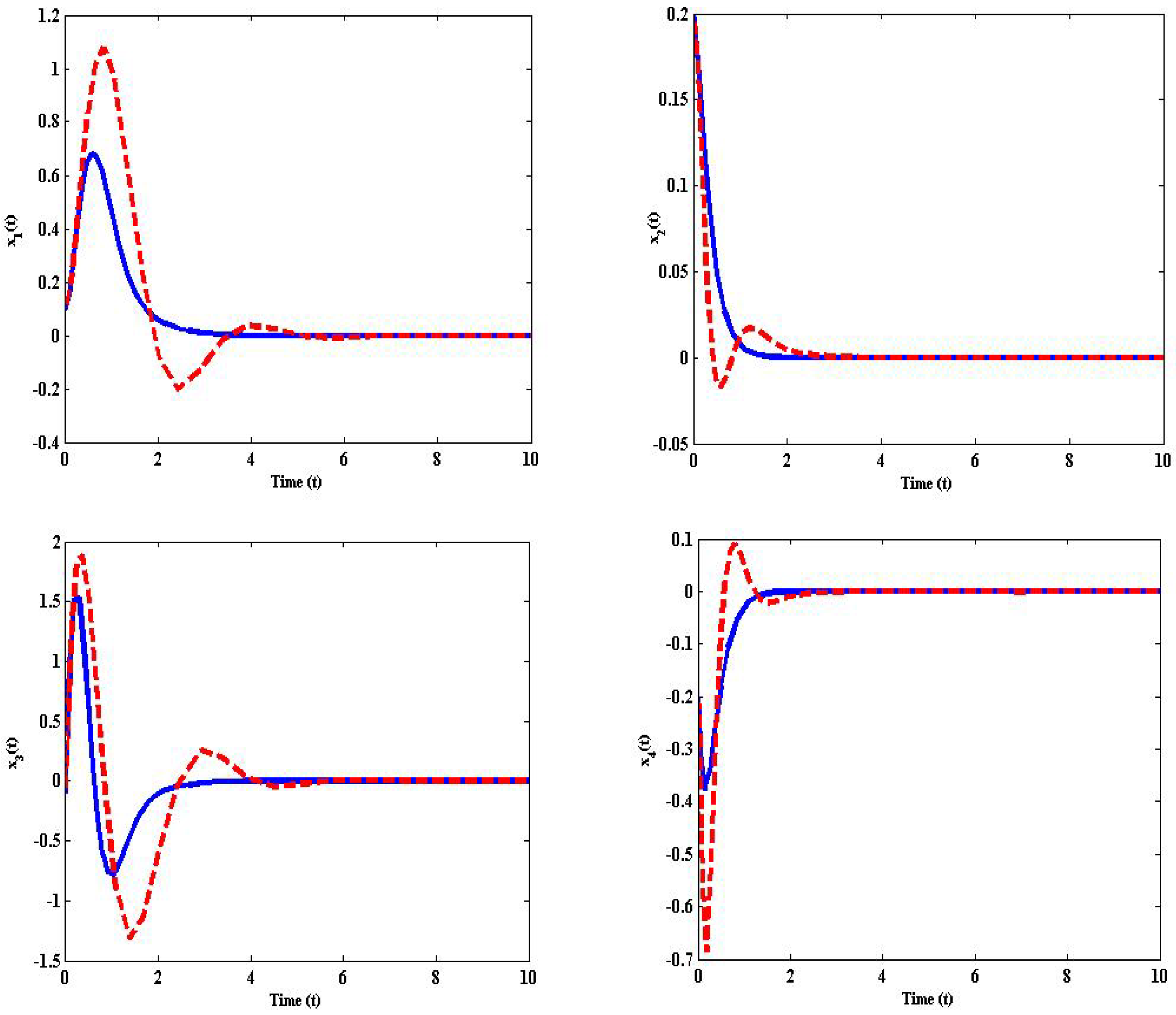
We set the disturbance input for the simulation environment as $w\left(t\right)=\frac{0.05}{1+t^2}$ for the initial condition $x\left(0\right)={\left[\begin{array}{cccc}0.1& 0.2& -0.1& -0.2\end{array}\right]}^T$. Figure 2 and Figure 3 present the simulation result for trajectories of displacement $x_1\left(t\right),x_2\left(t\right),x_3\left(t\right),x_4\left(t\right)$ and acceleration ${\ddot{x}}_1\left(t\right),{\ddot{x}}_2\left(t\right),{\ddot{x}}_3\left(t\right),{\ddot{x}}_4\left(t\right)$ of the controlled and uncontrolled nominal system (22) in the absence of uncertainty with the above control gain (66). Where the dark lines represent a closed loop system and the dashed lines indicate an open loop system. It is clear from Figure 2 and Figure 3 that the trajectories of the closed-loop nominal helicopter system converge fast to zero when compared to the open loop system. 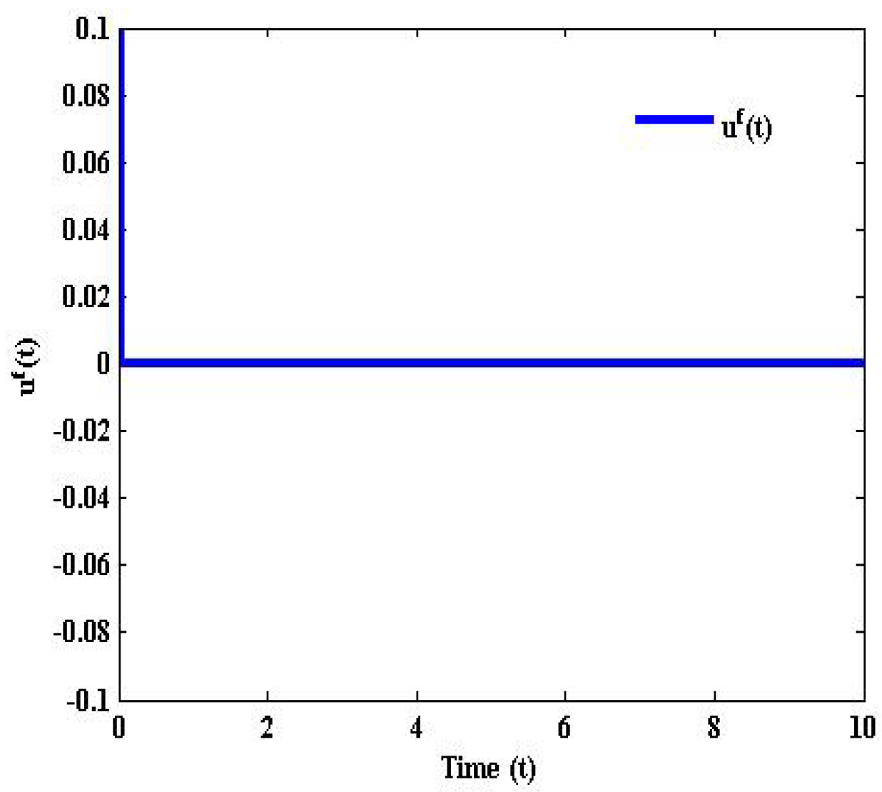Figure 4 depicts the time histories of the reliable control forces $u^f\left(t\right)$ operating on the helicopter system. 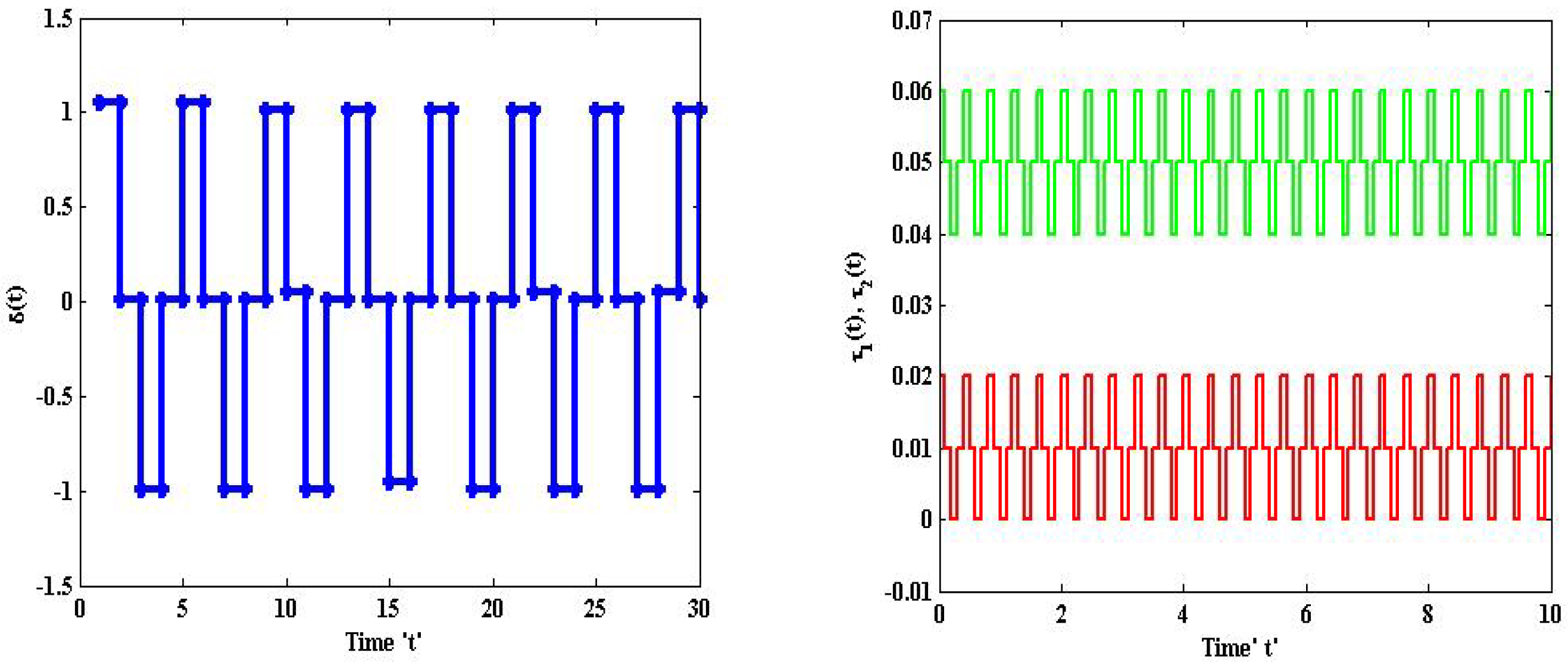Further, Figure 5 shows the Bernoulli random variable $\delta \left(t\right)$ and time-varying delay ${\tau }_1\left(t\right)\&{\tau }_2\left(t\right)$. The simulation results reveal that the considered sampled data reliable TS fuzzy helicopter system with mixed $H_{\infty }$ and a passivity performance attenuation level is stabilizable via the proposed state feedback control law.

 Case 2. 

The goal is now to build a robust state feedback reliable SDC utilizing a known actuator failure parameter matrix $G_1=G_2=0.7$ and the above-mentioned parameters, to ensure that the resultant closed loop system is robustly asymptotically stable.

For the satisfying time-varying delays ${\tau }_1\left(t\right)=0.01+0.01sin\left(\frac{\pi t}{2}\right)$ and ${\tau }_2\left(t\right)=0.03+0.03sin\left(\frac{\pi t}{2}\right)$, through solving the LMI requirements in Theorem 2, we provide the findings of the maximum acceptable delay bound $\overline{\tau }$ for distinct $\gamma$ in

Table 3. Maximum allowable $\overline{\tau }$ for various of $\gamma$ values in Case 2.

$\mathit{\gamma }$	0.1	0.3	0.4	0.5	0.7	0.9
$\overline{\tau }$	0.023	0.046	0.049	0.051	0.053	0.055

, by assuming ${\tau }_0=0.01,J=0.2,\beta =0.7,{\lambda }_1=0.4$ and ${\delta }_0=0.4$. Furthermore,

Table 4. Minimum $\gamma$ for various of $\overline{\tau }$ and J values in Case 2.

$\overline{\mathit{\tau }}$	0.02	0.03	0.04	0.05	0.06
$J=0.2$	0.2866	0.3745	0.4509	0.6522	1.6429
$J=0.7$	0.2867	0.3746	0.4512	0.6692	2.2502

shows the minimum guaranteed $H_{\infty }$ performance level $\gamma$ for various values of $\overline{\tau }$ and J.

Table 5. Minimum $\gamma$ for various of $\overline{\tau }$ and $\beta$ values in Case 2.

$\overline{\mathit{\tau }}$	0.03	0.04	0.05	0.06
$\beta =0$	0.5868	0.7034	0.8175	2.7521
$\beta =0.7$	0.3746	0.4512	0.6692	2.2502
$\beta =1$	0.3838	0.5432	0.8365	2.3376

also contains additional computational findings, including the minimum $\gamma$ for distinct values of $\overline{\tau }$ and $\beta .$

 Case 3. 

Our primary target is to create a reliable SDC so that, with all admissible uncertainties in addition to unknown actuator failures in the helicopter system model, the eventual results closed loop system (20) is robustly asymptotically stable and meets the MH_∞P performance level. Next, employing the same parameters as in Case 2, we examine the sensor fault matrix $G_{\eta },$ that satisfies $0.5\le G_{\eta }\le 0.9,$ and we may derive a feasible solution for Theorem 3.

Table 6. Minimum $\gamma$ for various of $\overline{\tau }$ and J values in Case 3.

$\overline{\mathit{\tau }}$	0.02	0.03	0.04	0.05
$J=0.2$	0.2863	0.3747	0.4515	0.8043
$J=0.9$	0.2867	0.3755	0.4559	2.1006

and

Table 7. Maximum allowable $\overline{\tau }$ for various of $\gamma$ and $\beta$ values in Case 3.

$\mathit{\gamma }$	0.2	0.25	0.3	0.035	0.4	0.5
$\beta =0$	0.017	0.019	0.022	0.024	0.026	0.030
$\beta =0.7$	0.030	0.035	0.039	0.041	0.042	0.044
$\beta =1$	0.028	0.030	0.032	0.033	0.035	0.037

illustrate that the calculated minimum guaranteed $H_{\infty }$ level $\gamma$ for different parameters of $\overline{\tau }$ & J and the derived upper bound of time delay $\overline{\tau }$ for various values of $\gamma$ and $\beta$.

Further, to show the effectiveness, the minimum MH_∞P performance for distinct values of $\overline{\tau }$ and $\beta$ is given in

Table 8. Minimum $\gamma$ for various of $\overline{\tau }$ and $\beta$ values in Case 3.

$\overline{\mathit{\tau }}$	0.03	0.035	0.04	0.045
$\beta =0$	0.5631	0.6490	0.6650	0.7652
$\beta =0.7$	0.3592	0.4142	0.5044	0.5115
$\beta =1$	0.4261	0.4763	0.7695	0.7810

.

For instance, if we set three different values of $\beta$ for $\gamma =0.5$ in Table 7, the corresponding gain matrices are obtained, as following three cases:

Rule 1: $H_{\infty }$ case—when $\beta =0$ the corresponding gain matrices are

$$\begin{array}{ccc}\hfill K_1& =& \left[\begin{array}{cccc}-0.0040& 1.4020& 0.0078& 0.4327\end{array}\right],K_2=\left[\begin{array}{cccc}-0.0137& 1.4023& 0.0080& 0.4426\end{array}\right],\hfill \\ \hfill K_3& =& \left[\begin{array}{cccc}-0.0214& 1.4002& 0.0082& 0.4460\end{array}\right].\hfill \end{array}$$

Rule 2: Passivity case—when $\beta =1$ the corresponding gain matrices are

$$\begin{array}{ccc}\hfill K_1& =& \left[\begin{array}{cccc}-0.0351& -0.2659& -0.0456& 0.0558\end{array}\right],K_2=\left[\begin{array}{cccc}-0.0980& -0.2450& -0.0454& 0.0575\end{array}\right],\hfill \\ \hfill K_3& =& \left[\begin{array}{cccc}-0.1658& -0.3200& -0.0469& 0.0504\end{array}\right].\hfill \end{array}$$

Rule 3: MH_∞P case—when $\beta =0.7$ the corresponding gain matrices are

$$\begin{array}{ccc}{K}_1& =& \left[\begin{array}{cccc}0.0170& 0.1364& -0.0162& 0.0846\end{array}\right],K_2=\left[\begin{array}{cccc}-0.0156& 0.1499& -0.0158& 0.0709\end{array}\right],\hfill \\ \hfill K_3& =& \left[\begin{array}{cccc}-0.0521& 0.0544& -0.0172& 0.0588\end{array}\right].\hfill \end{array}$$

(67)

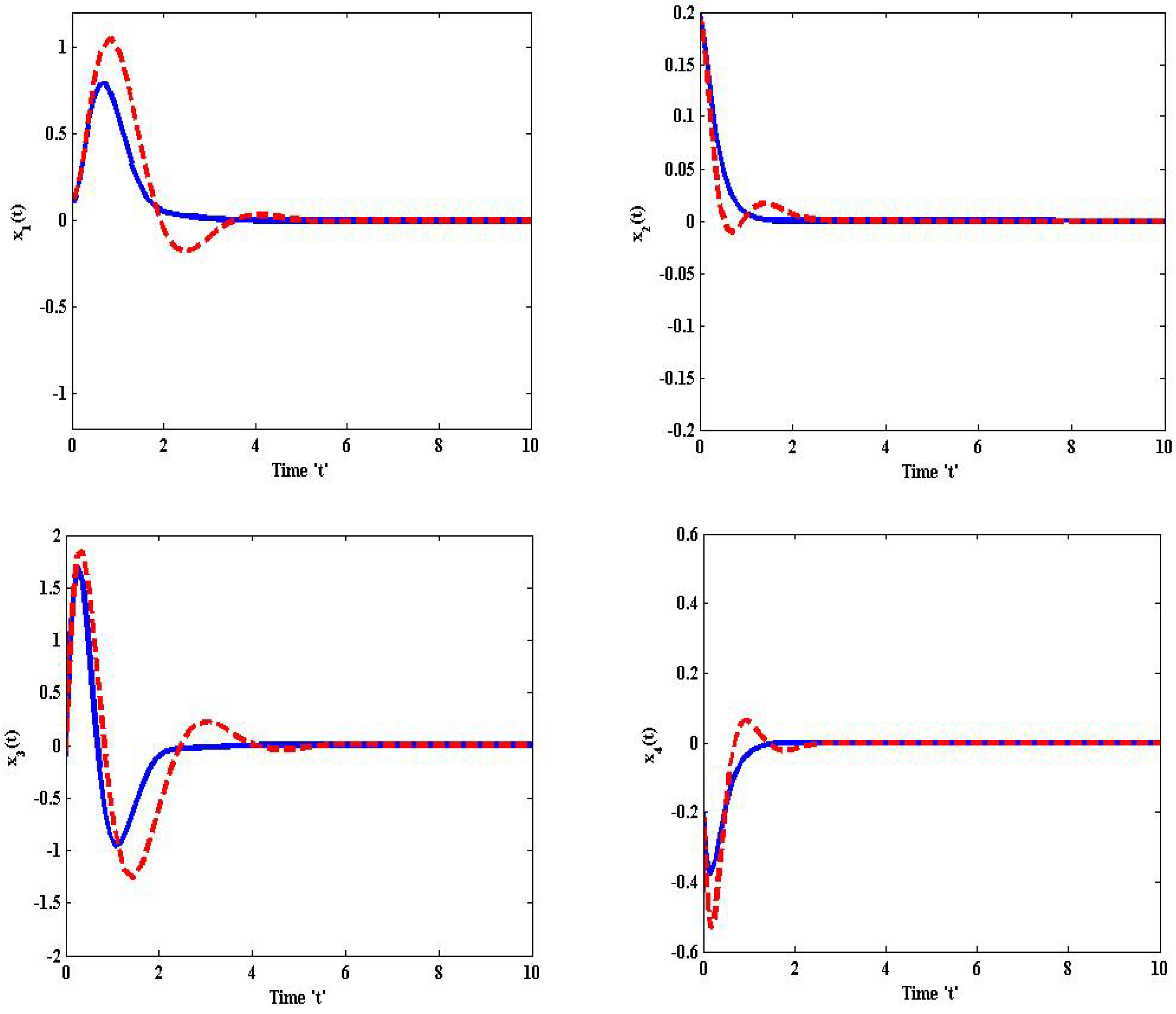
Figure 6 and Figure 7 represents the displacement $x_1\left(t\right),x_2\left(t\right),x_3\left(t\right),x_4\left(t\right)$ and acceleration ${\ddot{x}}_1\left(t\right),{\ddot{x}}_2\left(t\right),{\ddot{x}}_3\left(t\right),{\ddot{x}}_4\left(t\right)$ curves of the closed and open loop system as in the presence of uncertainties, in which the dark lines depict with control and the dashed lines indicate without control. Figure 8 represents the time responses of the robust reliable control input vector.

Figure 2, Figure 3, Figure 6 and Figure 7 show that the displacement and acceleration trajectories of the TS Fuzzy helicopter system converge faster to the equilibrium point when compared to the uncontrolled system, demonstrating the usefulness of our developed controller. The suggested reliable SDC with MH_∞P performance provides the system asymptotic stability with and without uncertainty. Thus, despite disturbances and uncertainties in the system model, the developed robust reliable sampled-data controller with random delay is effective and can stabilize the TS Fuzzy helicopter system.

 Remark 6. 

It is noted that from Table 1, Table 2, Table 5, Table 7 and Table 8, the mixed $H_{\infty }$ and passivity performance level as γ has better values than $\beta =0$ or 1. This shows that the mixed $H_{\infty }$ and passivity performance is better than the other two performances as $H_{\infty }$ performance and passive performance. As a result, the combined $H_{\infty }$ and passivity performance outperforms the other two.

In the following remarks, the proposed results in this paper have been compared with some existing ones.

 Remark 7. 

Consider that the sampled data helicopter system (63) and the parameters of each mode are the same as in the previous example.

One may easily acquire a feasible solution by solving the LMI in Corollary 1 using the MATLAB LMI tool box. It is clear that the delay-dependent stabilization result of the considered TS fuzzy Helicopter system, the computed maximum time delay τ and is displayed in

Table 9. Comparison table.

Gao and Chen [26]	Yoneyama [25]	Yoneyama [6]	Corollary 1
0.0072	0.0353	0.1890	0.2198

, which are compared with the results obtained in [6,25,26]. Our results are substantially less conservative than those of [6,25,26].

 Remark 8. 

The inverted pendulum’s system behavior is defined by the dynamic equation below [27,28].

$$\begin{array}{ccc}\hfill \ddot{\theta }\left(t\right)& =& \frac{gsin\left(\theta \left(t\right)\right)-a{m}_{p}L\dot{\theta }{\left(t\right)}^{2}sin\left(2\theta \left(t\right)\right)/2-acos\left(\theta \left(t\right)\right)u\left(t\right)}{4L/3-a{m}_{p}L{cos}^2\left(\theta \left(t\right)\right)}\hfill \end{array}$$

(68)

where $\theta \left(t\right)$ indicates the pendulum’s angular displacement, $g=9.8 m/s^2$ denotes gravity’s acceleration, $m_p\in \left[\begin{array}{cc}{m}_{pmin}& m_{pmax}\end{array}\right],=\left[\begin{array}{cc}2& 5\end{array}\right]kg$ denotes the pendulum’s mass, $m_c\in \left[\begin{array}{cc}{m}_{cmin}& m_{cmax}\end{array}\right],=\left[\begin{array}{cc}30& 35\end{array}\right]kg$ is the cart’s weight, $a=1/(m_p+M_c),2L=1 m$ is the pendulum length and $u\left(t\right)$ is the force applied to the cart. The system’s parameter uncertainties are represented by $m_p$ and $M_c.$ The inverted pendulum can indeed be described by the TS fuzzy model shown below:

$$\begin{array}{c}\hfill \begin{array}{ccc}\dot{x}\left(t\right)\hfill & =\hfill & {\displaystyle \sum _{\eta =1}^4}{\displaystyle \sum _{j=1}^4}{\lambda }_{\eta }\left(\xi \left(t\right)\right){\lambda }_j\left(\xi \left(t\right)\right)\left\{A_{\eta }x\left(t\right)+B_{\eta }{K}_{\eta }x(t-\tau \left(t\right))\right\}.\hfill \end{array}\end{array}$$

(69)

where $x\left(t\right)=\left[\begin{array}{cc}{x}_1\left(t\right)& x_2\left(t\right)\end{array}\right]=\left[\begin{array}{cc}{\theta }_1\left(t\right)& {\dot{\theta }}_2\left(t\right)\end{array}\right]$. For validating the performance analysis, we borrowed model parameters from [27,28], such as,

$$\begin{array}{ccc}\hfill A_1& =& A_2=\left[\begin{array}{cc}0& 1\\ f_{1min}& 0\end{array}\right],A_3=A_4=\left[\begin{array}{cc}0& 1\\ f_{1max}& 0\end{array}\right],B_1=B_3=\left[\begin{array}{cc}0& f_{1min}\end{array}\right],\hfill \\ \hfill B_2& =& B_4=\left[\begin{array}{cc}0& f_{2max}\end{array}\right],f_{1min}=11.3533,f_{1max}=16.4640,f_{2min}=-0.0192,\hfill \\ \hfill f_{2max}& =& -0.0492,\hfill \end{array}$$

The determined maximum upper bound $\tau$ is displayed in

Table 10. Comparison table.

Lam and Leung [27]	0.0662
Zhu and Wang (Corollary 2) [28]	0.0722
Zhu and Wang (Theorem 1) [28]	0.1093
Corollary 1	0.1232

for the Corollary 1. Furthermore, it is obvious from Table 10 that our highest upper bound is greater than the values in [27,28], implying that our results are substantially less conservative than [27,28].

5. Conclusions

The topic of the sampled-data reliable mixed $H_{\infty }$ and passivity-based control for a type of uncertain TS fuzzy CE151 helicopter system with LFT is studied in this work. A delay-dependent criteria for attaining the robust stabilization of uncertain TS fuzzy CE151 helicopter systems in the face of random delays and actuator defects is provided by creating a unique LKF. More precisely, the stabilizing conditions are stated in terms of solutions to a set of LMI that can be addressed effectively using a conventional LMI tool box. Finally, simulation results are shown to demonstrate the effectiveness and less conservative nature of the suggested control laws.