1. Introduction
Recently, multi-group models have gained more attention due to their wide range of applications in many different fields such as biology, epidemiology, etc. [
1,
2]. The different dynamical behaviors of multi-group models have been extensively investigated, see [
3,
4] for global stability, [
5] for synchronization and [
6] for stationary distribution.
Multiple dispersals have great influence in many multi-group models, especially in a multi-path environment, and different dispersal always exists among species. In addition, systems in nature are indispensable to be affected by stochastic perturbation [
7,
8,
9,
10]. Stochastic multi-group models with multiple dispersals are effective mathematical models and have attracted increasing attention, see [
11,
12,
13]. It should be noted that topological structures in many studies [
3,
4,
5,
6,
8,
9,
10,
11,
12,
13] are known. In fact, topological structures in many practical applications are usually unknown or uncertain. Therefore, it is important to identify the unknown topological structures of stochastic multi-group models with multiple dispersals.
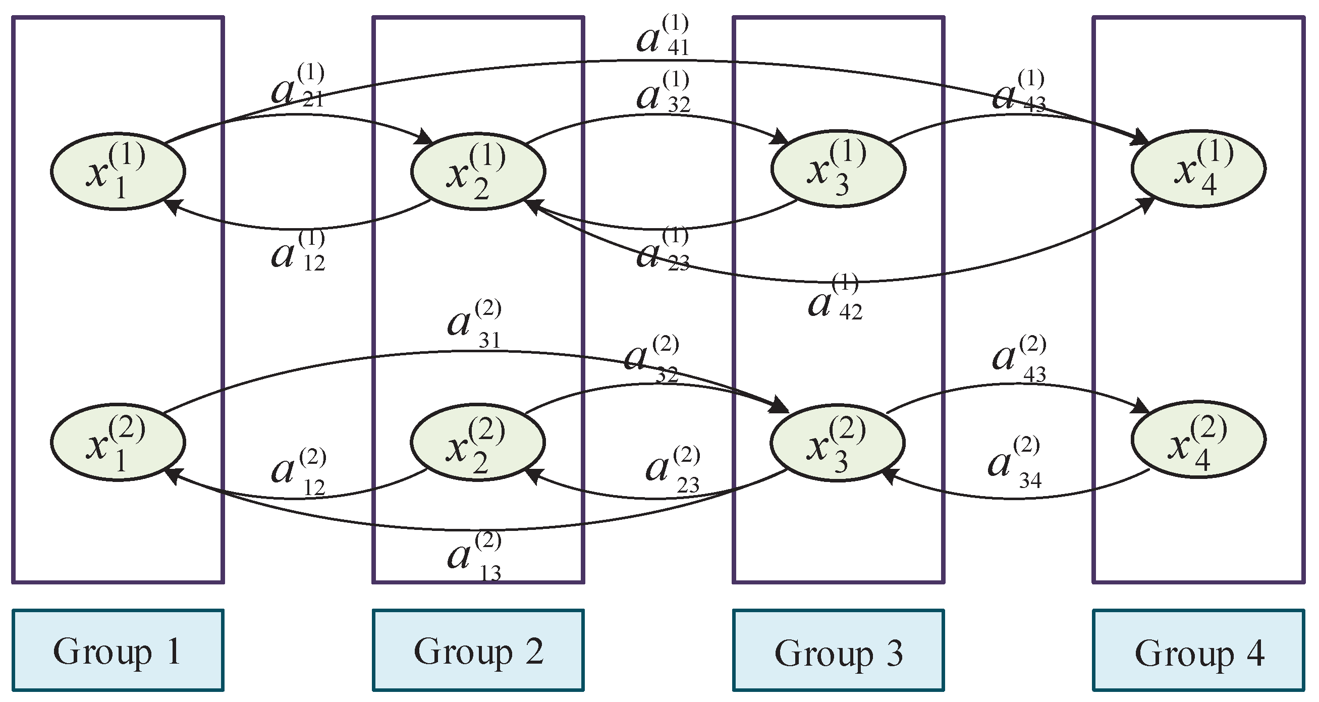
In this paper, we consider the following stochastic multi-group models with multiple dispersals as
where
is the state vector of the
i-th component in the
k-th group. We define
for
.
denotes the state vector of the
k-th group.
represents the performance of the
i-th component of the
k-th group.
shows the perturbation intensity on the
i-th component of the
k-th group.
means the dispersal rate of the
i-th component from the
h-th group to the
k-th group. Here,
iff there is no dispersal for the
i-th component from the
h-th group to the
k-th group.
is the influence of vertex
h on vertex
k,
is a one-dimensional Brownian motion. For better understanding, we draw a diagraph of four groups with two dispersals, see
Figure 1. Here,
,
In this paper, the mathematical models have a number of groups. If we add a controller to every group, it will result in high control cost. As is known, pinning control strategy is an effective technique to reduce the number of controlled groups [
14,
15,
16]. On the other hand, if a large number of groups have unknown partial topological structures or we are only interested in partial topological structures, then pinning control is an efficient technique. Therefore, we will try to use a pinning control mechanism to identify unknown partial topological structures of (
1).
It should be mentioned that the Lyapunov method is an efficient tool for studying partial topology identification [
17,
18,
19]. However, it is difficult to construct a suitable global Lyapunov function for (
1) due to multiple groups and dispersals. It is inspiring that Li and his co-authors have combined graph theory and the Lyapunov method to build a global Lyapunov function indirectly for coupled systems. At the same time, they use this method to study global stability of coupled systems [
20]. This method is called the graph-theoretic method. As far as we know, there are few works about partial topology identification of stochastic multi-group models via the graph-theoretic method.
Motivated by the above discussions, this paper aims to use the graph-theoretic method to identify unknown partial topological structures of stochastic multi-group models with multiple dispersals. The main contributions are as follows.
The mathematical model is general, which includes multiple dispersals and stochastic perturbation.
The pinning controller is cost-effective and can reduce controlled groups.
The graph-theoretic method for partial topology identification is novel.
The unknown partial topological structures of stochastic multi-group models with multiple dispersals can be identified successfully.
The remainder of this paper is organized as follows. In
Section 2, some preliminaries are displayed. The main results are introduced in
Section 3. In
Section 4, two numerical examples are used to verify the effectiveness of theoretical results. Conclusions are given in
Section 5.
2. Preliminaries
Some Necessary Basic Knowledge of Graph Theory and Stochastic Differential Equations
A directed graph contains a set of vertices and a set P of arcs , in which is the arc from initial vertex i to terminal vertex j. Given a digraph with N vertices, we define the weighted matrix whose entry equals the weight of arc if there is an arc from vertex i to vertex j, and 0 otherwise. The directed graph with weighted matrix U is described as . The Laplacian matrix of is defined as , where .
Suppose that the coefficients
and
of (
1) satisfy the local Lipschitz condition and the linear growth condition [
21,
22]. Then, for initial value
, (
1) has a unique continuous solution, which is denoted as
. Moreover, if
,
and
, then (
1) admits a trivial solution
.
We define the differential operator
acting on
along with the trajectories of (
1) as
where
, .
Lemma 1 ([
21]).
Assume that there is a function , a function and a continuous function such thatand the differential operator acting on V along with the trajectories of (1) satisfiesFurthermore, is bounded for . Then, for every initial value , exists and is almost surely finite. Moreover, Lemma 2 (Theorem 2.2 in [
20]).
Assume that . is the cofactor of the k-th diagonal element of . Then, the following identity holds:Here, are arbitrary functions, is the set of all spanning unicyclic graphs of , is the weight of , and denotes the directed cycle of
3. Main Results
In this section, we will study the problem of partial topology identification of stochastic multi-group models with multiple dispersals based on adaptive pinning synchronization and the graph-theoretic method.
In order to identify partial topological structures of stochastic multi-group models with multiple dispersals, taking (
1) as a drive system, the response system with an adaptive pinning controller is described as
and
are the perturbation intensity and function governing the dynamical behavior of the
i-th component of the
k-th group in the response network, respectively.
is the state vector of the
i-th component in the
k-th group.
denotes the state vector of the
k-th group.
represents the estimation of the unknown partial coupling matrix
.
is the general adaptive pinning controller. Without loss of generality, it is enough to identify partial topological structures of stochastic multi-group models with multiple dispersals consisting of the front
l groups and their dispersals, that is,
. Let
be the synchronization error, where
. We denote
. The dynamical system of synchronization error between systems (
1) and (
3) can be written as
where
.
Suppose that the following conditions hold for each and .
(A1) There are constants
such that the following inequality holds for any
:
(A2) Assume that
is bounded for
and there exists a constant
such that
(A3) There exist positive constants
and
such that
(A4) Suppose that for each and , are linearly independent on the orbit of the outer synchronization manifold
Next, we give some adaptive pinning controller and updating laws for
,
.
where
and
are arbitrarily positive constants.
Theorem 1. If (A1)–(A4) hold and is strongly connected for each , then the unknown partial topological structures of coupled network (1) can be identified by under the controller (5) and updating laws (6) with probability one. That is, it holds for each that Proof. We define
in which
is a large enough positive number. Then, it holds from the definition of differential operator
that
We define
where
is the cofactor of the
k-th diagonal element of the Laplacian matrix of
. Then, it is not difficult to derive that
Now, we calculate two parts,
I and
.
According to Lemma 2, it yields
where
is the set of all spanning unicyclic graphs of
,
is the weight of
and
means the directed cycle of
. Taking
it holds that
As
is large enough, there exists a
. Therefore,
where
is a constant determined by
and
. Furthermore, the above analysis implies that
Hence, from Lemma 1,
exists and is almost surely finite. It also holds that
By combining LaSalle’s invariance principle, assumption (A4) and error system (
4), one can obtain that the set
is the largest invariant set of
. Thus, for any initial value of error system (
4), the trajectory asymptotically converges to the
with probability one [
21]. It is proved that stochastic multi-group models with multiple dispersals (
1) and (
3) asymptotically achieve complete outer synchronization under an adaptive controller (
5) and updating laws (
6). Furthermore, the unknown multiple topological structures
have been successfully identified by
with probability one, which completes this proof. □
Remark 1. It is well-known that the Lyapunov method plays a significant role in the study of partial topology identification [17,18,19]. However, multiple dispersals and stochastic disturbances are considered in this paper, which makes mathematical models more complex. Hence, it is difficult to construct a global Lyapunov function directly for multi-group models. Motivated by [20,23,24], we construct a global Lyapunov function by the weighted summation of vertex Lyapunov functions in the form of . Here, is the cofactor of the k-th diagonal element of the Laplacian matrix of . Obviously, this method is closely related to topological structures of networks. It is always called the graph-theoretic method since this method uses some results of graph theory. The method can be applied to study dynamic behavior of many other networks. For example, in [20], the authors use the graph-theoretic method to study stability of single-species ecological models with dispersal. The global-stability result they obtained is stronger than those in [25,26]. Moreover, the global asymptotic stability of coupled oscillators and multi-patch predator–prey models can also be obtained by using the graph-theoretic method. Remark 2. Though the adaptive control method can realize topology identification of multi-group models, it needs to add a controller to every group [27,28]. However, in this paper, the model includes a great number of groups. Adding controllers to all groups is sometimes difficult to implement and the control costs may be higher. Therefore, the proposed pinning control of this paper is useful. On the one hand, it can reduce control costs because only a small fraction of groups need to be controlled. On the other hand, it is more feasible that one can only add controllers to groups of interest to identify the corresponding unknown topological structures. When
, we can obtain the whole topology identification. In detail, the corresponding response system of drive system (
1) can be characterized by
Then, the error system between drive system (
1) and response system (
10) can be denoted by
The adaptive controller and updating laws for
are given as follows:
where
are arbitrarily positive constants. Then, we obtain the following corollary.
Corollary 1. If (A1)–(A4) hold and is strongly connected for each , then the unknown whole topological structures of coupled network (1) can be identified by under the controller (12) and updating laws (13). That is, it holds for each that The proof is similar to Theorem 1 and we omit it here.
If
, then the corresponding whole topology identification result can be found in [
27]. Therefore, the mathematical model of this paper is more general. Moreover, theoretical results of this paper are common, where both partial topology identification and whole topology identification can be obtained.
4. Simulation Results
In this section, two simulation examples are given to verify the validity of theoretical results. We use the Lorenz system to describe the dynamic of each group. Obviously, the Lorenz system satisfies (A1) [
29].
Example 1. We consider a general coupled systems with four groups and three kinds of diffusion. The drive system can be put into the following form:where . , ;
, ;
, .
Some weights of configuration matrices can be arbitrarily selected as
the other values are set as 0. Without loss of generality, we add controllers to the first two groups. Then, we only need to identify partial weight configuration matrices Accordingly, the response system with an adaptive pinning controller can be denoted by
We define
Then, the error system between (
14) and (
15) can be shown as
Available from Theorem 1, three weight configuration matrices
can be estimated by
under the following controller and updating laws for
.
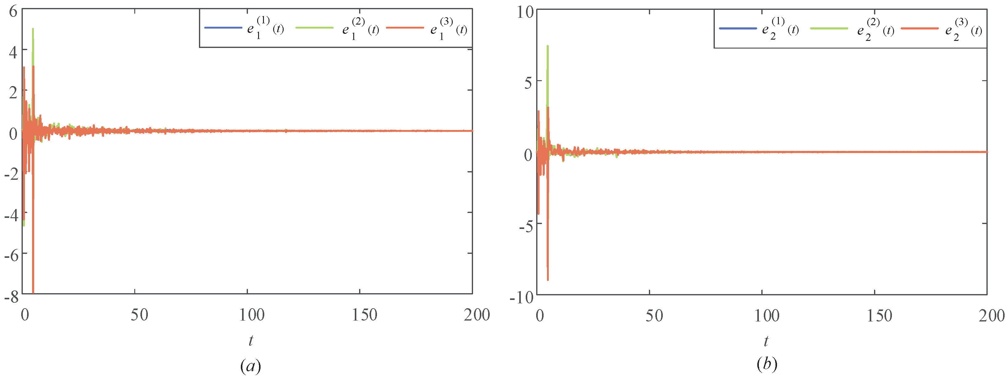
Taking
we can obtain some simulations. The synchronization error for drive system (
14) and response system (
15) are shown in
Figure 2.
Figure 2a shows the synchronization error of the first group and
Figure 2b shows the synchronization error of the second group. Apparently, all of the error curves approach 0 over time, which means the drive–response systems can reach synchronization.
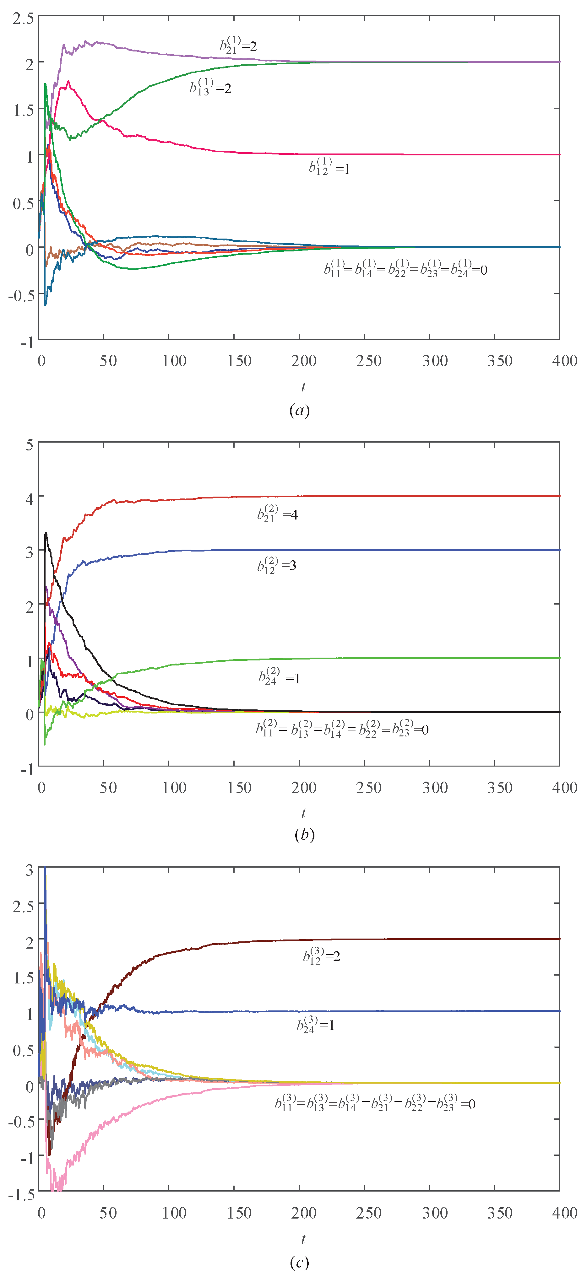
Figure 3 gives time evolution of
in system (
15).
Figure 3a shows the identification results of
. It is observed that the curves stabilize at three constants: 2 for
and
, 1 for
and 0 for
.
Figure 3b shows the identification results of
. One can see that
tends to 4,
tends to 3,
tends to 1 and
tend to 0.
Figure 3c shows the identification results of
. As we can see, curve
converges to 2, curve
converges to 1 and curves
converge to 0. Therefore, all of the curves of
can converge to a real value, which implies the partial topology identification is successful.
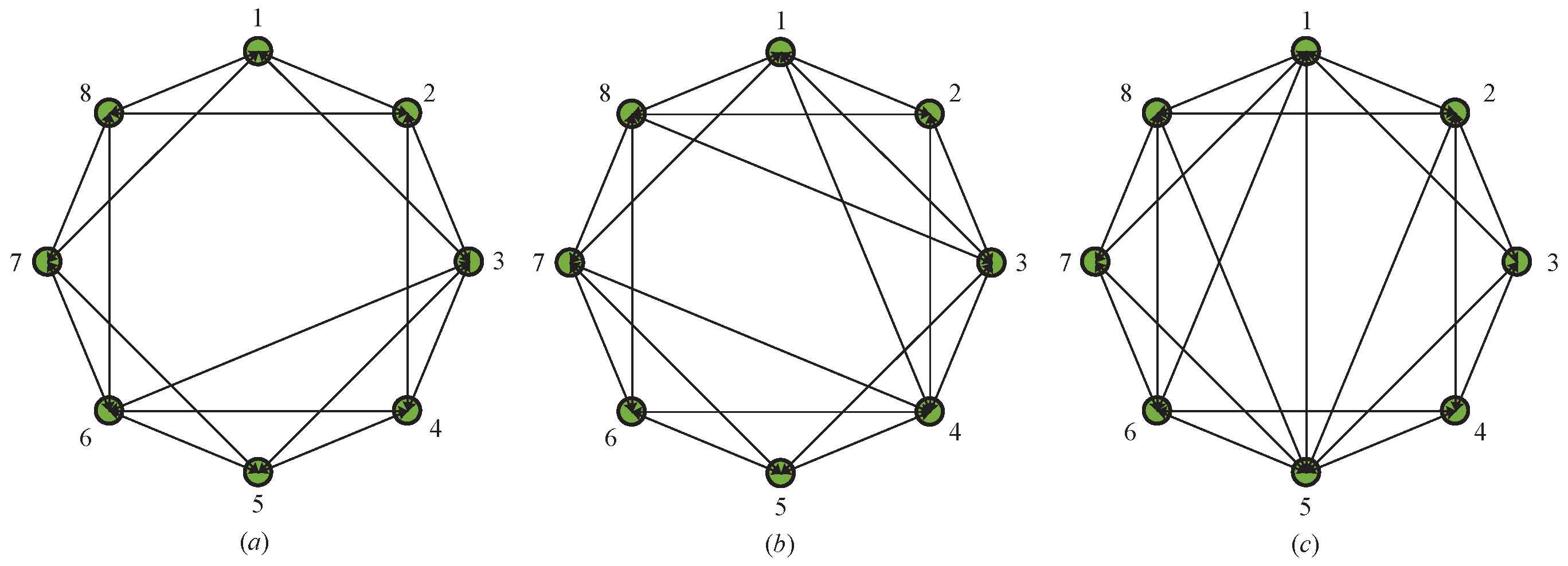
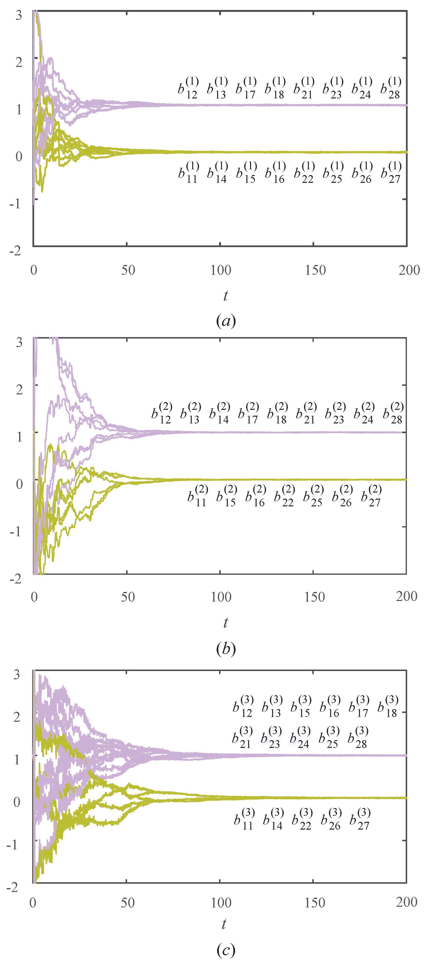
Example 2. In this example, we suppose that the network structure obeys the small-world algorithm proposed by Newman and Watts [30]. Consider system (14) consisting of eight groups and the number of pinned groups is the same as the above example. For a better view, the topological structures are demonstrated in Figure 4, in which Figure 4a obeys the small-world algorithm with parameters , Figure 4b obeys the small-world algorithm with parameters , Figure 4c obeys the small-world algorithm with parameters . Therein, The other . Moreover, some parameters are arbitrarily set as follows: The other parameters are the same as the above example.
Under the same conditions as the above example, one can obtain that all assumptions of Theorem 1 are satisfied. This implies that three weight configuration matrices
can be estimated by
under the controller and updating laws (
17) and (
18) for
.
Figure 5 shows the simulation results of
. It is obvious that all curves stabilize at real values, which means the partial topology identification is successful.


