Adaptive Intelligent High-Order Sliding Mode Fractional Order Control for Harmonic Suppression

Abstract

A second-order sliding mode control (SOSMC) with a fractional module using adaptive fuzzy controller is developed for an active power filter (APF). A second-order sliding surface using a fractional module which can decrease the discontinuities and chattering is designed to make the system work stably and simplify the design process. In addition, a fuzzy logic control is utilized to estimate the parameter uncertainties. Simulation and experimental discussion illustrated that the designed fractional SOSMC with adaptive fuzzy controller is valid in satisfactorily eliminating harmonic, showing good robustness and stability compared with an integer order one.

1. Introduction

One of the most prominent contributions of the second industrial revolution is the invention of electrical appliances. With the development of our society, the usage of electronic equipment has become quite common and has brought great convenience to our life. Non-linear loads generate negative effects for power quality and harmonic. Electricity is essential in modern society and widely used in fields with growing electric power demand. However, with the more and more complex environment of the grid, grid harmonic pollution has become increasingly serious, which will increase power loss of the grid and degrade the power quality. Therefore, harmonic suppression has become an important means to improve the efficiency of industrial production and ensure the normal and stable operation of a power system. Therefore, the various methods of harmonic suppression in a power grid have become a research hotspot in recent years. The most common method of harmonic suppression is to install filtering devices in the power system to filter out harmonics. APF is a type of power electronic equipment that can actively and efficiently compensate harmonics. It possesses the merits of having large frequency range, fast response speed and high compensation accuracy compared to passive filters, and APF has been widely applied in electricity, transportation, new energy and other fields. Faced with serious load increase and sudden voltage change, APF can compensate the harmonic current by tracking the reference current quickly and accurately in the presence of valid controllers [1,2].

At present, APF control strategies mainly have a hysteresis controller, single-cycle controller, or triangular wave controller. The advantage of sliding mode control (SMC) [3,4,5] is robustness to external disturbances as well as with changes and uncertainties of internal parameters. Therefore, the sliding mode control method is very suitable for APF current control, which is difficult to model and requires high control accuracy. Recently, intelligent controllers such as neural approximator [6,7,8] and fuzzy system [9,10] have been effective ways to deal with the model uncertainty in APF.

Fractional order control [11,12,13,14,15] can increase the degree of freedom of parameter adjustment, improve the flexibility of controller design and the accuracy of the system, and it has been widely implemented in various nonlinear systems. The fractional-order integrator and differentiator could give an extra degree of freedom, and the energy transfer under fractional order is slower than that with an integer order one, reducing the chattering. Sliding mode control [16,17,18] and terminal sliding mode control [19,20] can be combined with intelligent methods to improve the dynamic performance of active power filters, permanent magnet linear synchronous motors, robot manipulators, and micro gyroscopes. By differentiating, a new sliding surface is constituted to be a second-order sliding mode control (SOSMC), reducing chattering effectively [21,22,23,24,25]. SOSMC have been widely used in robot manipulators [21], buck DC-DC converters [22], active power filters [23] and doubly-fed induction generators [24,25].

However, a comprehensive method which combines fuzzy control, fractional-order control and SOSMC has not been designed for harmonic suppression. In the sliding mode control schemes for the power quality control issue, neither of them have used second-order control to eliminate chattering or used fractional order control to improve control accuracy. Therefore, an adaptive fractional SOSMC with fuzzy approximator is investigated for the control of the APF. The main properties of the proposed controller are highlighted as:

(1) SOSMC is utilized to remove the discontinuities and reduce chattering to develop a smoother controller. It is applied with a fractional fuzzy controller to increase the performance and robustness properties of the system.

(2) The adaptive intelligent fuzzy controller is then used to approximate lumped uncertain terms, thereby contributing to a fuzzy-based approximator by adding a fractional sliding mode and developing parameter updating laws.

(3) A fractional-order SOSMC is designed by combining a fuzzy controller with a fractional-order (FO) calculus, increasing tracking accuracy and convergence rate. The system with fractional modules could have an additional degree of freedom compared with integer orders.

2. Mathematical Model of APF

The circuit model of a typical three-phase APF is shown in Figure 1, and mainly includes three components: grid voltage, non-linear load and APF main circuit. The core devices of the APF main circuit are IGBTs which is a kind of switching devices with high voltage resistance and fast switching frequency. Moreover, the nonlinear load is acted upon by an uncontrollable rectifier bridge with capacitive load. The main circuit consisting of power switching devices produces compensation currents according to the control signal from the control system. In order to eliminate harmonic component, the compensation currents should be the same magnitudes and opposite phases with the harmonic currents.

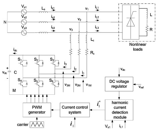
Figure 1. Schematic structure of an APF.

From Kirchhoff"s laws, circuit equations can be obtained as:

$$\left\{\begin{array}{l}{v}_1=L_c\frac{d{i}_1}{dt}+R_c{i}_1+v_{1M}+v_{MN}\\ v_2=L_c\frac{d{i}_2}{dt}+R_c{i}_2+v_{2M}+v_{MN}\\ v_3=L_c\frac{d{i}_3}{dt}+R_c{i}_3+v_{3M}+v_{MN}\end{array}\right.$$

(1)

where $v_1$, $v_2$, $v_3$ are the voltages of public join points, $i_1$, $i_2$, $i_3$ are the compensation current of APF, $L_c$ is an inductance, $R_c$ is a resistance and $v_{MN}$ is the voltage between M and N.

Summing (1), and assuming no zero-sequence and balanced supply voltages, then we get:

$$v_{MN}=-\frac{1}{3}{\displaystyle \sum _{m=1}^3{v}_{mM}}$$

(2)

The switching function of $c_k$ means the ON/OFF status in the two legs of the IGBT bridge, expressed as

$$c_k=\left\{\begin{array}{l}1\begin{array}{cc}& if{S}_{k}isonand{S}_{k+3}isoff\end{array}\\ 0\begin{array}{cc}& if{S}_{k}isoffand{S}_{k+3}ison\end{array}\end{array}\right.$$

(3)

where k = 1, 2, 3…….

Define $v_{km}=c_k\cdot v_{dc}$, and Equation (1) is expressed as:

$$\left\{\begin{array}{c}\frac{d{i}_1}{dt}=-\frac{R_c}{L_c}{i}_1+\frac{v_1}{L_c}-\frac{v_{dc}}{L_c}{(\mathrm{c}}_1-\frac{1}{3}{\displaystyle \sum _{m=1}^3{c}_m})\\ \frac{d{i}_2}{dt}=-\frac{R_c}{L_c}{i}_2+\frac{v_2}{L_c}-\frac{v_{dc}}{L_c}{(\mathrm{c}}_2-\frac{1}{3}{\displaystyle \sum _{m=1}^3{c}_m})\\ \frac{d{i}_3}{dt}=-\frac{R_c}{L_c}{i}_3+\frac{v_3}{L_c}-\frac{v_{dc}}{L_c}{(\mathrm{c}}_3-\frac{1}{3}{\displaystyle \sum _{m=1}^3{c}_m})\end{array}\right.$$

(4)

The switching state $d_{nk}$ is denoted as

$$d_k=c_k-\frac{1}{3}{\displaystyle \sum _{m=1}^3{c}_m}$$

(5)

Hence $d_{nk}$ is determined by $c_k$.

From the permissible eight switching states of IGBT, we obtain

$$\left[\begin{array}{c}{d}_1\\ d_2\\ d_3\end{array}\right]=\frac{1}{3}\left[\begin{array}{ccc}2& -1& -1\\ -1& 2& -1\\ -1& -1& 2\end{array}\right]\left[\begin{array}{c}{c}_1\\ c_2\\ c_3\end{array}\right]$$

(6)

Then Equation (4) is expressed as

$$\left\{\begin{array}{l}\frac{d{i}_1}{dt}=-\frac{R_c}{L_c}{i}_1+\frac{v_1}{L_c}-\frac{v_{dc}}{L_c}{d}_1\\ \frac{d{i}_2}{dt}=-\frac{R_c}{L_c}{i}_2+\frac{v_2}{L_c}-\frac{v_{dc}}{L_c}{d}_2\\ \frac{d{i}_3}{dt}=-\frac{R_c}{L_c}{i}_3+\frac{v_3}{L_c}-\frac{v_{dc}}{L_c}{d}_3\end{array}\right.$$

(7)

Then the dynamic model is expressed as

$$\dot{x}=f\left(x\right)+\mathit{bu}+h_k$$

(8)

where $x$ equals to $i_1$, $i_2$ or $i_3$, $f(x)=\frac{R_c^{}}{L_c^{}}{i}_k+\frac{v_k}{L_c}$, $b=-\frac{v_{dc}}{L_c}$, $u=\frac{v_{dc}}{L_c}{(\mathrm{c}}_k-\frac{1}{3}{\displaystyle \sum _{m=1}^3{c}_m})$, $h_k$ is an unknown and bounded disturbance.

3. Design of Adaptive Fractional Second-Order Sliding Mode Fuzzy Control

Firstly, the sliding surface of the SOSMC is proposed, then the controller with the parameter adaptive laws are derived. The block diagram of the proposed control system for APF is shown in Figure 2. The control goal is to design a control system to achieve the aim that the compensation current $y$, that is, the output current of APF, tracks reference current $x_d$.

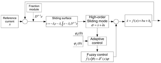
Figure 2. Structure chart for control system.

The tracking error is expressed in (9), where $x_d$ denotes an ideal current, command current is $x$.

$$e=x_d-x$$

(9)

The derivative of Equation (9) is:

$$\dot{e}={\dot{x}}_d-f(x)-bu-h_k$$

(10)

Define ${}_{a}D{}_t^{\alpha }$ as a fundamental operator, where $\alpha$ is t fractional order, $t,a$ are the operation"s bounds. We use $D^{\alpha }$ to replace ${}_{a}D{}_t^{\alpha }$ to simply the derivation.

Design a sliding surface with a fractional order component as:

$$s=-{\lambda }_{1}e-{\lambda }_2{\displaystyle \int e-{\lambda }_3{D}^{\alpha -1}e}$$

(11)

where ${\lambda }_1,{\lambda }_2,{\lambda }_3>0$, the fractional order is $\alpha -1$.

Then the derivative of Equation (11) is derived as:

$$\dot{s}=-{\lambda }_1\dot{e}-{\lambda }_{2}e-{\lambda }_3{D}^{\alpha }e$$

(12)

Substituting derivative of sliding surface as Equation (10) into Equation (12) gets

$$\dot{s}=-{\lambda }_1({\dot{x}}_d-f(x)-bu-h_k)-{\lambda }_{2}e-{\lambda }_3{D}^{\alpha }e$$

(13)

Define high order sliding surface $\sigma =\dot{s}+\partial s$, where $\partial >0$, then substituting Equation (13) into $\sigma =\dot{s}+\partial s$ obtains

$$\sigma =-{\lambda }_1{\dot{x}}_d+{\lambda }_{1}f(x)+{\lambda }_{1}bu+{\lambda }_1{h}_k-{\lambda }_{2}e-{\lambda }_3{D}^{\alpha }e-\partial {\lambda }_{1}e-\partial {\lambda }_2{\displaystyle \int e-\partial {\lambda }_3{D}^{\alpha -1}e}$$

(14)

The derivative of Equation (14) becomes:

$$\dot{\sigma }=-{\lambda }_1{\ddot{x}}_d+{\lambda }_1\dot{f}(x)+{\lambda }_{1}b\dot{u}+{\lambda }_1{\dot{h}}_k-{\lambda }_2\dot{e}-{\lambda }_3{D}^{\alpha +1}e-\partial {\lambda }_1\dot{e}-\partial {\lambda }_{2}e-\partial {\lambda }_3{D}^{\alpha }e$$

(15)

where ${\dot{d}}_k$ is the derivative of $d_k$.

Setting $\dot{\sigma }=0$, then solve an equivalent controller as:

$${\dot{u}}_{eq}=\frac{1}{b{\lambda }_1}({\lambda }_1{\ddot{x}}_d-{\lambda }_1\dot{f}(x)-{\lambda }_1{\dot{h}}_k+{\lambda }_2\dot{e}+{\lambda }_3{D}^{\alpha +1}e+\partial {\lambda }_1\dot{e}+\partial {\lambda }_{2}e+\partial {\lambda }_3{D}^{\alpha }e)$$

(16)

Then hitting controller $u_{sw}$ is designed as $u_{sw}=\rho \mathrm{sgn}(\sigma )$, a new controller is designed as:

$$\dot{u}=\frac{1}{b{\lambda }_1}\left({\lambda }_1{\ddot{x}}_d-{\lambda }_1\dot{f}(x)+({\lambda }_2+\partial {\lambda }_1)({\dot{x}}_d-f(x)-bu)-\rho \mathrm{sgn}(\sigma )+{\lambda }_3{D}^{\alpha +1}e+\partial {\lambda }_{2}e+\partial {\lambda }_3{D}^{\alpha }e\right)$$

(17)

Substituting (17) and (10) into (15) yields

$$\dot{\sigma }={\lambda }_1{\dot{d}}_k+({\lambda }_2+\partial {\lambda }_1)h_k-\rho \mathrm{sgn}(\sigma )$$

(18)

A Lyapunov function is chosen as $V_1=\frac{1}{2}{\sigma }^T\sigma$

Then:

$$\begin{array}{l}{\dot{V}}_1={\sigma }^T\left({\lambda }_1{\dot{d}}_k+({\lambda }_2+\partial {\lambda }_1)h_k-\rho \mathrm{sgn}(\sigma )\right)\\ \begin{array}{cc}& \end{array}\le {\sigma }^T\left|{\lambda }_1{\dot{d}}_k+({\lambda }_2+\partial {\lambda }_1)h_k\right|-\rho \left|\sigma \right|\end{array}$$

(19)

While $\rho \ge {\left|{\lambda }_1{\dot{h}}_k+({\lambda }_2+\partial {\lambda }_1)h_k\right|}_{\max }$, ${\dot{V}}_1\le 0$, where ${\left|{\lambda }_1{\dot{h}}_k+({\lambda }_2+\partial {\lambda }_1)h_k\right|}_{\max }$ is the maximum value of ${\lambda }_1{\dot{h}}_k+({\lambda }_2+\partial {\lambda }_1)h_k$.

Then we design fuzzy systems $\widehat{f}(x_k),\widehat{h}({\sigma }_k)$ to estimate $f(x_k),\rho \mathrm{sgn}({\sigma }_k)$, where ${\sigma }_k$ is the scalar component of $\sigma$,$k=1,2,3$. Therefore, an updated controller with a fuzzy approximator is expressed as:

$$u=\frac{1}{b{\lambda }_1}\left({\lambda }_1{\ddot{x}}_d-{\lambda }_1\dot{\widehat{f}}(x)+({\lambda }_2+\partial {\lambda }_1)({\dot{x}}_d-f(x)-bu)-\widehat{h}({\sigma }_k)+{\lambda }_3{D}^{\alpha +1}{e}_k+\partial {\lambda }_2{e}_k+\partial {\lambda }_3{D}^{\alpha }{e}_k\right)$$

(20)

where: $\widehat{f}(x_k\left|{\theta }_{fk}^{*}\right.)-\widehat{f}(x_k)={\delta }^T(x_k){\phi }_{fk}$,$\widehat{h}({\sigma }_k\left|{\theta }_{hk}^{*}\right.)-\widehat{h}({\sigma }_k\left|{\theta }_{hk}\right.)={\varphi }^T(h_k){\phi }_{hk}$, ${\delta }^T(x_k),{\varphi }^T(h_k)$ are fuzzy vectors. ${\phi }_{fk}^{}$ ${\phi }_{hk}^{}$ are the designed adaptive laws as:

$${\dot{\phi }}_{fk}=-{[1+{\gamma }_1{\sigma }_k{\lambda }_1{({\phi }_{fk}{\phi }_{fk}^T)}^{-1}{\phi }_{fk}{\delta }^T(x_k)]}^{-1}{({\phi }_{fk}{\phi }_{fk}^T)}^{-1}{\phi }_{fk}({\gamma }_1{\sigma }_k{\lambda }_1{\dot{\delta }}^T(x_k){\phi }_{fk}-{\gamma }_1{\sigma }_k({\lambda }_2+\partial {\lambda }_1){\delta }^T(x_k){\phi }_{fk})$$

(21)

$${\dot{\phi }}_{hk}=-{\gamma }_2{\sigma }_k{({\phi }_{hk}{\phi }_{hk}^T)}^{-1}{\phi }_{hk}{\varphi }_{hk}^T{\phi }_{hk}$$

(22)

where ${\gamma }_1>0,{\gamma }_2>0$.

Theorem 1.

The controller as in Equation (20) and adaptive laws as in Equations (21) and (22) are derived to ensure that the signal$x$tracks the reference signal$x_d$, and the${\theta }_f(t)$and${\theta }_h(t)$are bounded and stable.

Proof. 

Define the parameters as:

$${\theta }_f^{*}=\arg \underset{{\theta }_f\in {\Omega }_f}{\min }[\sup |\widehat{f}(x|\underset{x\in R^n}{{\theta }_f})-f(x)|]$$

(23)

$${\theta }_h^{*}=\arg \underset{{\theta }_h\in {\Omega }_h}{\min }[\sup |\widehat{h}(\sigma |\underset{x\in R^n}{{\theta }_h})-\rho \mathrm{sgn}(\sigma )|]$$

(24)

where ${\Omega }_f$ and ${\Omega }_h$ denote the aggregation of ${\theta }_f$ and ${\theta }_h$, $\sup f(x)$ is the minimum value of upper bound for $f(x)$ and $\arg (\min f(x))$ is the set value of $x$ with the largest value of $f(x)$.

A minimum estimation error is denoted as

$$\omega =f(x)-\widehat{f}(x|{\theta }_f^{*})$$

(25)

where $\omega$ is upper bounded by a positive value ${\omega }_{\max }$ as $\left|\omega \right|\le {\omega }_{\max }$.

When $\theta$ obtains the optimal parameter of ${\theta }_h^{*}$, $\widehat{h}$ becomes:

$$\widehat{h}({\sigma }_k\left|{\theta }_{hk}^{*}\right.)=(\rho +\eta )\mathrm{sgn}(\sigma )$$

(26)

where $\eta \ge 0$.

Then Equation (15) is obtained as:

$$\begin{array}{cc}\hfill \dot{\sigma }& ={\lambda }_1(\dot{f}(x_k)-\dot{\widehat{f}}(x_k))+({\lambda }_2+\partial {\lambda }_1)(f(x_k)-\widehat{f}(x_k))-\widehat{h}({\sigma }_k)+{\lambda }_1{\dot{h}}_k+({\lambda }_2+\partial {\lambda }_1)h_k\hfill \\ & ={\lambda }_1(\widehat{\dot{f}}(x_k|{\theta }_{fk}^{*})-\dot{\widehat{f}}(x_k)+\dot{f}(x_k)-\widehat{\dot{f}}(x_k|{\theta }_{fk}^{*}))\hfill \\ & +({\lambda }_2+\partial {\lambda }_1)(\widehat{f}(x_k|{\theta }_{fk}^{*})-\widehat{f}(x_k)+f(x_k)-\widehat{f}(x_k|{\theta }_{fk}^{*}))\hfill \\ & +\widehat{h}({\sigma }_k|{\theta }_{sk}^{*})-\widehat{h}({\sigma }_k|{\theta }_{sk}^{})-\widehat{h}({\sigma }_k|{\theta }_{sk}^{*})+{\lambda }_1{\dot{h}}_k+({\lambda }_2+\partial {\lambda }_1)h_k\hfill \end{array}$$

(27)

where $\widehat{f}(x_k\left|{\theta }_{fk}^{*}\right.)-\widehat{f}(x_k)={\delta }^T(x_k){\phi }_{fk},\widehat{h}({\sigma }_k\left|{\theta }_{hk}^{*}\right.)-\widehat{h}({\sigma }_k\left|{\theta }_{hk}\right.)={\varphi }^T(h_k){\phi }_{hk}$ $k=1,2,3$.

Design a Lyapunov function candidate as:

$$\begin{array}{cc}\hfill V_2& =V_1+\frac{1}{2{\gamma }_1}({\phi }_{fk}^T{\phi }_{fk}+{\phi }_{hk}^T{\phi }_{hk})\hfill \\ & {}_{}=\frac{1}{2}{\sigma }^T\sigma +\frac{1}{2{\gamma }_1}({\phi }_{fk}^T{\phi }_{fk}+{\phi }_{hk}^T{\phi }_{hk})\hfill \end{array}$$

(28)

The derivative of $V_2$ is:

$${\dot{V}}_2={\sigma }^T\dot{\sigma }+\frac{1}{{\gamma }_1}{\phi }_{fk}^T{\dot{\phi }}_{fk}+\frac{1}{{\gamma }_2}{\phi }_{hk}^T{\dot{\phi }}_{hk}$$

(29)

Taking Equation (27) into Equation (29) yields:

$$\begin{array}{cc}\hfill {\dot{V}}_2=& \frac{1}{{\gamma }_1}[{\gamma }_1{\sigma }_k{\lambda }_1{\delta }^T(x_k){\dot{\phi }}_{fk}+{\gamma }_1{\sigma }_k{\lambda }_1{\dot{\delta }}^T(x_k){\phi }_{fk}+{\gamma }_1{\sigma }_k({\lambda }_2+\partial {\lambda }_1){\delta }^T(x_k){\phi }_{fk}+{\phi }_{fk}^T{\dot{\phi }}_{fk}]\hfill \\ & +\frac{1}{{\gamma }_2}[{\gamma }_2{\sigma }_k({\lambda }_2+\partial {\lambda }_1){\varphi }_{hk}^T{\phi }_{hk}+{\phi }_{hk}^T{\dot{\phi }}_{hk}]+{\sigma }_k({\lambda }_2+\partial {\lambda }_1)[{\omega }_k+d_k-\widehat{h}({\sigma }_k|{\theta }_{hk}^{*})]+{\sigma }_k{\lambda }_1{\dot{\omega }}_k\hfill \end{array}$$

(30)

Because ${\dot{\phi }}_{fk}=-{\dot{\theta }}_{fk}$, ${\dot{\phi }}_{hk}=-{\dot{\theta }}_{hk}$, $\widehat{h}({\sigma }_k\left|{\theta }_{hk}^{*}\right.)=(\eta +\rho )\mathrm{sgn}({\sigma }_k)$,

Substituting (21), (22) into (30) obtains

$$\begin{array}{cc}\hfill {\dot{V}}_2& ={\sigma }_k[{\lambda }_1{\dot{h}}_k+({\lambda }_2+\partial {\lambda }_1)h_k+({\lambda }_2+\partial {\lambda }_1){\omega }_k-(\eta +\rho )\mathrm{sgn}({\sigma }_k)]\hfill \\ & \le {\sigma }_k[({\lambda }_2+\partial {\lambda }_1){\omega }_k-\eta \mathrm{sgn}({\sigma }_k)]\hfill \\ & \le ({\lambda }_2+\partial {\lambda }_1){\sigma }_k{\omega }_k-\eta \left|{\sigma }_k\right|\hfill \\ & \le \left|{\sigma }_k\right|(({\lambda }_2+\partial {\lambda }_1)\left|{\omega }_k\right|-\eta )\hfill \end{array}$$

(31)

If $\eta \ge ({\lambda }_2+\partial {\lambda }_1)·\left|{\omega }_{k\max }\right|$,$\left|{\omega }_{k\max }\right|$ is maximum value of ${\omega }_k$, ${\dot{V}}_2\le 0$. According to Barbalart lemma, ${\omega }_k$,$\eta$ and $\sigma$ all can converge to zero. □

4. Experiment Verification

4.1. Simulation Study

In this part, simulation results using Matlab/Simulink and SimPower Toolbox are accomplished to demonstrate the advantages of the proposed method. In the simulation process, the CPU is i5-8300H (2.30 GHz), the system is 64-bit, and the version of MATLAB is 2019b. The control task is to design the controller to output an appropriate duty cycle to control the correct switching of the IGBT according to the calculated reference current, so as to realize the high-precision tracking control task of the current.

The selection of these values is directly related to the performance improvement of the controller. The parameters of Table 1 are determined in the following rule. DC link voltage and capacitance: The DC side of the active power filter normally uses a DC capacitor instead of the DC power supply as an energy storage device. Since the text adopts the low-voltage $U_s=24\mathrm{V}$ design scheme, after comprehensive consideration this paper finally selects the DC side voltage as 50 since the larger the capacitor value that is selected, the more favorable it is for the DC side voltage regulation. Therefore, combined with the actual test effect, this paper finally selects the DC side capacitor value as $C=2200\mathsf{\mu }\mathrm{F}$. Since the APF in this paper is a low-voltage system, this paper requires $\Delta i_{\max }=0.1\mathrm{A}$. In the end, the minimum value of the AC inductance can be obtained as $L_{\min }\approx 5.6\mathrm{m}\mathrm{H}$. Combined with the actual simulation effect, this paper finally chose the inductance value $L=10\mathrm{m}\mathrm{H}$.

Table 1. APF model parameters.

Parameters	Values
Supply voltage	Us = 24 V; f = 50 Hz
Steady load	R1 = 5 Ω, R2 = 15 Ω, C = 1 × 10−3 F
Dynamic load	R1 = 15 Ω, R2 = 15 Ω, C = 1 × 10−3 F
APF main circuit parameters	Rc = 0.1 Ω, Lc = 10 mH, $C=2.2\times {10}^{-3}\mathrm{F},U_{dc}^{*}$ = 50 V
Sample time	Ts = 5 × 10−5 s

The membership functions are selected as f:

$\mu =\exp (-{[x+5-1.99·(i-1)]}^2)$, $i=1,\mathrm{...6}$, where $i$ means the number for fuzzy rules; 36 fuzzy rules can be obtained to estimate the unknown system if $i=6$. The member function graph is shown in Figure 3.

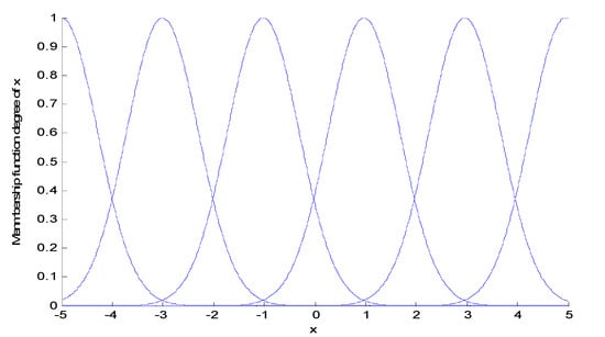
Figure 3. The member function graph of $x$.

$r_1=3000,r_2=450,\partial =\mathrm{36,000},b=\mathrm{130,000}$, ${\lambda }_1=0.00000005$, ${\lambda }_2=0.00646$, ${\lambda }_3={10}^{-15}$. A rectifier bridge attached with parallel RC road is chosen as nonlinear load, PI control with $k_p=0.03$, $k_i=0$ is chosen for DC voltage.

Figure 4, Figure 5 and Figure 6 give the tracking property for reference and compensation current using different fractional orders. If $\alpha =0.2$, the compensation current does not track the reference current as in Figure 4. However, if $\alpha =0.4$ the reference current could be tracked before 0.09 s. After changing $\alpha$ to 0.8, the reference current could be accurately and quickly tracked. Therefore, tracking property becomes better by increasing the value of $\alpha$. Then we select $\alpha =0.8$ to obtain better results. Figure 7 is a source and load current graph. Load was added into the circuit at 0.1 s and 0.2 s step by step, the load current will change with the load changes. Before APF begins to take action at 0.04 s, there is not any difference. After APF began to take action, source current was slightly varying; however, it converges to a sine wave quickly and stably even with changing load. In Figure 8, DC side voltage with the proposed method in this paper rapidly increased; there are vibrations with changing load, but it keeps stable finally.

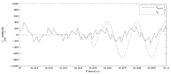
Figure 4. Target and compensation current using fractional order when $\alpha =0.2$.

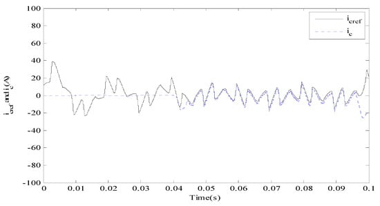
Figure 5. Target and compensation current using fractional order $\alpha =0.4$.

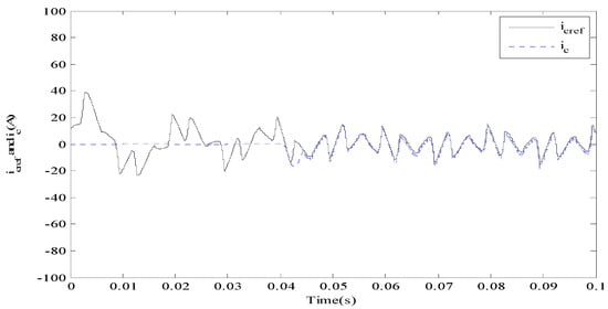
Figure 6. Target and compensation current using fractional order $\alpha =0.8$.

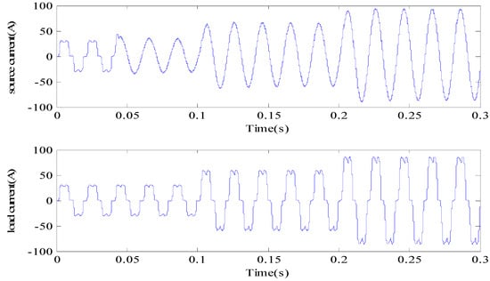
Figure 7. Source and load current with fractional order control.

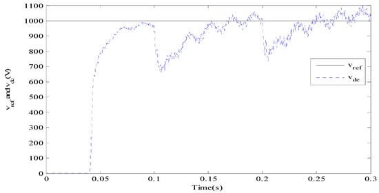
Figure 8. DC side voltage with fractional order control.

Figure 9 plots the tracking error for the compensation current with the proposed fractional order controller. The tracking error in the current using fractional order control is small, showing that the fractional order method has better effects on compensation current tracking. Table 2 gives a comparison of the values of mean square error among three different controllers:

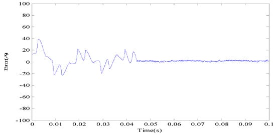
Figure 9. Compensation current tracking error with fractional order control.

Table 2. Comparative MSE values among three different controllers.

	Mean Square Error	Adaptive Fuzzy Sliding Mode Control	Integer Order SOSMC Fuzzy Control	Fractional Order SOSMC Fuzzy Control
$\mathit{\alpha }$
$\alpha =0.8$		1.9023	1.6058	1.1919

Table 2 presents values of mean square error (MSE) among three different controllers. Start time is chosen from 0.04 s when APF starts to work, and the MSE of the proposed method is smaller than the other two methods, demonstrating that the proposed scheme has a better tracking effect.

Figure 10 shows the total harmonic distortion (THD) at the start point. Figure 11, Figure 12 and Figure 13 show the THD"s value after APF works at 0.06 s, 0.16 s and 0.26 s, respectively. In order to show the good properties of the designed controller, a comparison of the THD values among three different controllers is given in Table 3. As illustrated by Table 2, the THDs of both controllers are lower than 4%, but values of THD for the proposed scheme are lower than the other two controllers, proving that fractional order control and SOSMC could improve performance significantly.

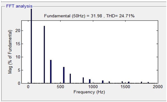
Figure 10. Harmonic spectrum of source current at 0 s.

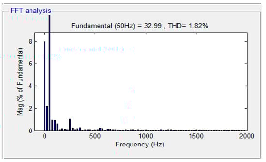
Figure 11. Harmonic spectrum of source current at 0.06 s.

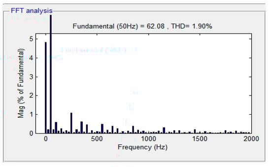
Figure 12. Harmonic spectrum of source current at 0.16 s.

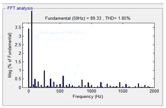
Figure 13. Harmonic spectrum of source current at 0.26 s.

Table 3. The comparison of values of THD among three different controllers.

	THD	Adaptive Fuzzy Sliding Mode Control	Integer Order SOSMC Fuzzy Control	Fractional Order SOSMC Fuzzy Control
Time (s)
0 s		24.71	24.71	24.71
0.06 s		2.56	2.14	1.82
0.16 s		2.29	1.98	1.90
0.26 s		1.99	1.93	1.85

4.2. Experiment Set-Up

According to Figure 1, a single-phase prototype of APF is built as in Figure 14. In addition to the APF parts, there are the signal collecting circuit, current control system, insulated gate bipolar transistor (IGBT) drive and pulse width modulation (PWM) generator. The signal collecting circuit first collects (1) load current, (2) compensation current, (3) power supply voltage, and (4) DC-side capacitor voltage, and then transmits these signals to the control system (in the dSPACE DS1104) through the A/D conversion unit. Then the controller transmits the PWM signal. Finally, the drive circuit drives the IGBT switch for current compensation.

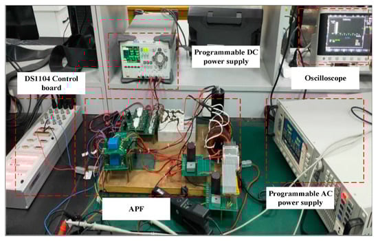
Figure 14. Experimental prototype structure.

The parameters in the experiment are the same as in Table 1 in the simulation.

Figure 15 and Figure 16 show the experimental results with the increased nonlinear load. The system has performance at fast speed with the THD value of 8.21%. Finally, Figure 17 and Figure 18 show the experimental results with the decreased nonlinear load, where the THD is 9.74%. The experimental results show that the compensation performance of APF is good in dynamic conditions, which also proves the feasibility of the proposed control method.

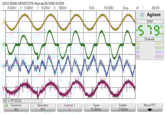
Figure 15. Dynamic-state oscilloscope waveform after the load increases.

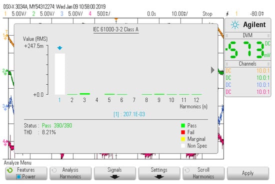
Figure 16. Dynamic-state THD rate after the load increases.

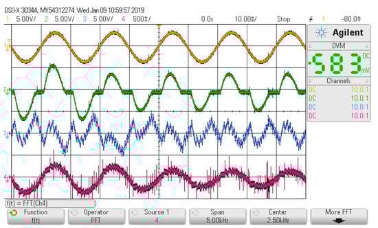
Figure 17. Dynamic-state oscilloscope waveform after load reduction.

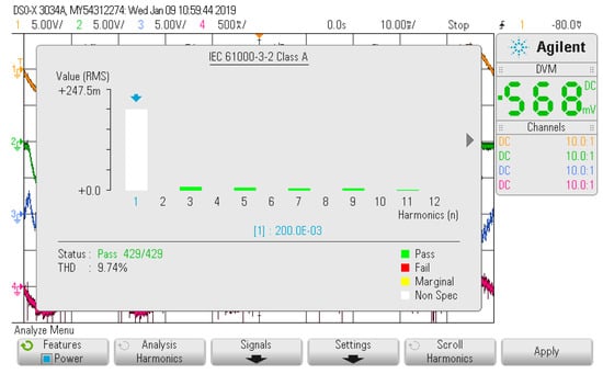
Figure 18. Dynamic-state THD rate after the load reduction.

It shows that the method still has excellent control performance in the case of sudden load changes, which reflects the robustness and adaptive ability of the proposed method. It can be seen from the experimental results that the proposed method has the advantages of being accurate, fast and highly adaptive at the same time and has high practical significance.

5. Conclusions

In this research, an FO-SOSMC is investigated to obtain harmonic current compensation and achieve a sinusoidal-type grid current, and to regulate and balance the voltage across the DC bus capacitor. A fractional-order SOSMC is designed by combining a fuzzy controller with a fractional-order (FO) calculus, increasing tracking accuracy and convergence rate. A fuzzy controller is designed to estimate the unknown term in the fractional order SOSMC and decrease chattering using a SOSMC. In this method, the use of fractional-order SMC allows the system to reach a steady state for a limited time and allows the sliding mode surface to quickly converge to zero in a finite time. The fuzzy controller whose parameters can be adjusted adaptively according to the adaptive laws can realize on-line accurate estimation of the unknown model of APF system.

Simulation and experiment demonstrate that the designed method has small tracking error and good THD. The values of THD for the proposed scheme are lower than for the other two controllers, proving that fractional order control and SOSMC could improve performance significantly. Experimental validation by implementing the proposed method on an actual three-phase APF system in real-time is needed in the next research steps. Considering the superior control performance, the presented approach can be further extended to other power electronic controls

References

- Thao, N.; Uchida, K.; Kofuji, K.; Jintsugawa, T.; Nakazawa, C. An Automatic-Tuning Scheme Based on Fuzzy Logic for Active Power Filter in Wind Farms. IEEE Trans. Control Syst. Technol. 2019, 27, 1694–1702. [Google Scholar] [CrossRef]
- Fei, J.; Wang, Z.; Pan, Q. Self-Constructing Fuzzy Neural Fractional-Order Sliding Mode Control for Active Power Filter. IEEE Trans. Neural Netw. Learn. Syst. 2022, 1–12. [Google Scholar] [CrossRef]
- Ray, A.; Bhattacharya, A. Improved Tracking of Shunt Active Power Filter by Sliding Mode Control. Int. J. Electr. Power Energy Syst. 2016, 78, 916–925. [Google Scholar]
- Pradhan, R.; Subudhi, B. Double Integral Sliding Mode MPPT Control of a Photovoltaic System. IEEE Trans. Control Syst. Technol. 2016, 24, 285–292. [Google Scholar] [CrossRef]
- Baek, J.; Jin, M.; Han, S. A New Adaptive Sliding-Mode Control Scheme for Application to Robot Manipulators. IEEE Trans. Ind. Electron. 2016, 63, 3628–3637. [Google Scholar] [CrossRef]
- Hamad, M.; Gadoue, S.; Williams, B.W. Harmonic Compensation of a Six-Pulse Current Source Controlled Converter using Neural Network-Based Shunt Active Power Filter. IET Power Electron. 2012, 5, 747–754. [Google Scholar] [CrossRef]
- Wai, R.; Lin, Y.; Liu, Y. Design of Adaptive Fuzzy-Neural-Network Control for a Single-Stage Boost Inverter. IEEE Trans. Power Electron. 2015, 30, 7282–7298. [Google Scholar] [CrossRef]
- Fei, J.; Liu, L. Real-Time Nonlinear Model Predictive Control of Active Power Filter Using Self-Feedback Recurrent Fuzzy Neural Network Estimator. IEEE Trans. Ind. Electron. 2022, 69, 8366–8376. [Google Scholar] [CrossRef]
- Khanesar, M.; Oniz, Y.; Kaynak, O.; Gao, H. Direct Model Reference Adaptive Fuzzy Control of Networked SISO Nonlinear Systems. IEEE/ASME Trans. Mechatron. 2016, 21, 205–213. [Google Scholar]
- Sahraei, B.; Shabaninia, F.; Nemati, A.; Stan, S. A Novel Robust Decentralized Adaptive Fuzzy Control for Swarm Formation of Multiagent Systems. IEEE Trans. Ind. Electron. 2012, 59, 3124–3134. [Google Scholar] [CrossRef]
- Lopes, A.; Machado, J. Fractional-Order Sensing and Control: Embedding the Nonlinear Dynamics of Robot Manipulators into the Multidimensional Scaling Method. Sensors 2021, 21, 7736. [Google Scholar] [CrossRef] [PubMed]
- Chen, T.; Cheng, J. On the Algorithmic Stability of Optimal Control with Derivative Operators. Circuits Syst. Signal Process. 2020, 39, 5863–5881. [Google Scholar] [CrossRef]
- David, S.; Fischera, C.; Machado, J. Fractional electronic circuit simulation of a nonlinear macroeconomic model. AEU-Int. J. Electron. Commun. 2018, 84, 210–220. [Google Scholar] [CrossRef]
- Muthukumar, P.; Balasubramaniam, P.; Ratnavelu, K. Sliding mode control design for synchronization of fractional order chaotic systems and its application to a new cryptosystem. Int. J. Dyn. Control 2017, 5, 115–123. [Google Scholar] [CrossRef]
- Han, Z.; Li, S.; Li, H. Composite learning sliding mode synchronization of chaotic fractional-order neural network. J. Adv. Res. 2020, 25, 87–96. [Google Scholar] [CrossRef] [PubMed]
- Fei, J.; Wang, Z.; Fang, Y. Self-Evolving Chebyshev Fuzzy Neural Fractional-Order Sliding Mode Control for Active Power Filter. IEEE Trans. Ind. Inform. 2022. [Google Scholar] [CrossRef]
- Chen, S.; Chiang, H.; Liu, T.; Chang, C. Precision Motion Control of Permanent Magnet Linear Synchronous Motors Using Adaptive Fuzzy Fractional-Order Sliding-Mode Control. IEEE/ASME Trans. Mechatron. 2019, 24, 741–752. [Google Scholar] [CrossRef]
- Fei, J.; Wang, Z.; Liang, X.; Feng, Z.; Xue, Y. Adaptive Fractional Sliding Mode Control of Micro Gyroscope System Using Double Loop Recurrent Fuzzy Neural Network Structure. IEEE Trans. Fuzzy Syst. 2022, 30, 1712–1721. [Google Scholar] [CrossRef]
- Wang, Z.; Fei, J. Fractional-Order Terminal Sliding Mode Control Using Self-Evolving Recurrent Chebyshev Fuzzy Neural Network for MEMS Gyroscope. IEEE Trans. Fuzzy Syst. 2022, 30, 2747–2758. [Google Scholar] [CrossRef]
- Wang, Y.; Gu, L.; Xu, Y.; Cao, X. Practical Tracking Control of Robot Manipulators With Continuous Fractional-Order Nonsingular Terminal Sliding Mode. IEEE Trans. Ind. Electron. 2016, 63, 6194–6204. [Google Scholar] [CrossRef]
- Ferrara, A.; Incremona, G.P. Design of an Integral Suboptimal Second-Order Sliding Mode Controller for the Robust Motion Control of Robot Manipulators. IEEE Trans. Control Syst. Technol. 2015, 23, 2316–2325. [Google Scholar] [CrossRef]
- Ling, R.; Shu, Z.; Hu, Q.; Song, Y. Second-Order Sliding-Mode Controlled Three-Level Buck DC-DC Converters. IEEE Trans. Ind. Electron. 2018, 65, 898–906. [Google Scholar] [CrossRef]
- Fei, J.; Li, S. Adaptive Fractional High Order Sliding Mode Fuzzy Control of Active Power Filter. In Proceedings of the 2018 Joint 10th International Conference on Soft Computing and Intelligent Systems and 19th International Symposium on Advanced Intelligent Systems, Toyama, Japan, 5–8 December 2018; pp. 576–580. [Google Scholar]
- Evangelista, C.; Pisano, A.; Puleston, P.; Usai, E. Receding Horizon Adaptive Second-Order Sliding Mode Control for Doubly-Fed Induction Generator Based Wind Turbine. IEEE Trans. Control Syst. Technol. 2017, 25, 73–84. [Google Scholar] [CrossRef]
- Martinez, M.; Susperregui, A.; Zubia, I.; Tapia, G. Design and Tuning of Fixed-Switching-Frequency Second-Order Sliding-Mode Controller for Doubly Fed Induction Generator Power Control. IET Electr. Power Appl. 2012, 6, 696–706. [Google Scholar]
Publisher"s Note: MDPI stays neutral with regard to jurisdictional claims in published maps and institutional affiliations. |
© 2022 by the authors. Licensee MDPI, Basel, Switzerland. This article is an open access article distributed under the terms and conditions of the Creative Commons Attribution (CC BY) license (https://creativecommons.org/licenses/by/4.0/).