
Cluster Oscillation of a Fractional-Order Duffing System with Slow Variable Parameter Excitation


1
Department of Mathematics and Physics, Shijiazhuang Tiedao University, Shijiazhuang 050043, China
2
Department of Mechanical Engineering, Shijiazhuang Tiedao University, Shijiazhuang 050043, China
3
State Key Laboratory of Mechanical Behavior and System Safety of Traffic Engineering Structures, Shijiazhuang Tiedao University, Shijiazhuang 050043, China
*
Author to whom correspondence should be addressed.
Fractal Fract. 2022, 6(6), 295; https://doi.org/10.3390/fractalfract6060295
Submission received: 17 April 2022
/
Revised: 18 May 2022
/
Accepted: 25 May 2022
/
Published: 28 May 2022
(This article belongs to the Special Issue Application of Fractional Calculus as an Interdisciplinary Modeling Framework)
Abstract
:The complicated dynamic behavior of a fractional-order Duffing system with slow variable parameter excitation is investigated. The stability and bifurcation behavior of the fast subsystem are analyzed by using the dynamic theory of fractional-order systems. The pitchfork bifurcation, Hopf bifurcation and limit cycle bifurcation are discussed in detail, and it was found that Hopf bifurcation only happens while the fractional order is bigger than 1. On the other hand, the influence of the amplitude of parametric excitation on cluster oscillation models is discussed. The results show that amplitude regulates cluster oscillation models with different bifurcation types. The point–point cluster oscillation only relates to pitchfork bifurcation. The point–cycle cluster oscillation includes pitchfork bifurcation and Hopf bifurcation. The point–cycle–cycle cluster oscillation involves three kinds of bifurcation, i.e., the pitchfork bifurcation, Hopf bifurcation and limit cycle bifurcation. The larger the amplitude, the more bifurcation types are involved. The research results of cluster oscillation and its generation mechanism will provide valuable theoretical basis for mechanical manufacturing and engineering practice.
1. Introduction
A Duffing system is obtained from a simple physical model. As a typical nonlinear system, many nonlinear oscillation problems can be transformed into a Duffing system in engineering, such as the destruction of chemical bonds, ship rolling motion and structural oscillation. As the fractional-order calculus possesses memory [1] and nonlocality in time and space, it has been widely applied in engineering vibration problems. Numerous scholars have paid attention to fractional-order Duffing system due to its abundant vibration behaviors. In recent years, related stability, analytical solution, numerical solution, bifurcation and control have been widely studied. For instance, Simo et al. [2] considered the effects of fractional order on the antiperiodic oscillations in a forced Duffing equation. Shen et al. [3,4,5] discussed various resonance forms and analytical solutions of a fractional-order Duffing oscillator. Nguyen et al. [6] investigated the subharmonic resonance of a Duffing oscillator with a fractional-order derivative and analyzed its stability. In reference [7,8], the fractional-order Duffing system was investigated by a numerical method. The bifurcation behavior of a fractional-order Duffing system was studied, and its rich nonlinear behavior was found [9,10,11,12]. For example, Li et al. [9] studied static bifurcation in a fractional-order delay Duffing system with asymmetric potential. The period-doubling bifurcation of a stochastic fractional-order Duffing system with a bounded random parameter subject to harmonic excitation was investigated [10]. Liu et al. [11] analyzed the global bifurcations of a fractional-order Duffing system. The nonlinear dynamic behaviors of a Duffing system with a fixed fractional order were investigated by using bifurcation diagrams, phase portraits, Poincare maps and time domain waveforms [12]. In engineering fields, the related control function of a fractional-order Duffing system was investigated [13,14].
The coupling phenomenon of multiple scales widely exists in biology, chemistry, mechanical engineering and other fields [15,16,17,18], which makes the dynamic behavior of the nonlinear system more complicated. The multiple scale coexistence of the system may derive from the enormous gap between different internal parameters or the different frequencies. In general, there are three forms of vibration in coupled systems with different scales, such as spiking state (SP), quiescence state (QS) and cluster oscillation. When the state variable is in large-amplitude oscillations, it is called SP. When it is in small-amplitude oscillations, it corresponds to the quiescent state and recorded as QS. When the trajectory moves back and forth between SP and QS, it is called cluster oscillation. Based on a system with different scales, some scholars have carried out in-depth research on various clustering behaviors in many fields. Lin et al. [19] designed a simple autonomous three-element-based memristive circuit with slow–fast effects and analyzed the complex dynamical behaviors. Zhang et al. [20] used the Adams–Bashforth–Moulton algorithm to study the dynamic evolution behavior of the hydro-turbine governing system, which contributes to the optimization analysis and control of the practical process. Lu et al. [21] investigated a variety of neuron models by using of slow–fast analysis method and analyzed their cluster oscillations and bifurcation behavior. Han and Bi et al. [22] analyzed the Duffing system with multi-frequency parametric excitation and found rich clustering modes.
The vibration phenomenon of parametric excitation systems is more complicated in the engineering field. Based on the above introduction, there is little work on the cluster oscillation of a fractional-order Duffing system with a slow variable parameter excitation, especially on multiple time scales. In fact, its dynamic behavior is more abundant. Therefore, this paper focuses on the fractional-order Duffing system with a slow variable parameter excitation. The rest of this paper is organized as follows. In Section 2, we consider the stabilities and bifurcations of the fractional-order Duffing system. The generation mechanism of cluster oscillation and the influence of the amplitude of parametric excitation are discussed in Section 3. Section 4 contains some conclusions.
2. Bifurcation Analysis
If the stiffness of the fractional-order Duffing system is subjected to periodic excitation, the corresponding motion equation becomes
where is the derivative of on and is the damping ratio. and are the excitation amplitude and frequency, respectively. When , Equation (1) is a slow–fast coupling system with a two time-scale. The definition of Caputo fractional derivative [23] was adopted.
where and . is a Gamma function satisfying .
In order to separate the fast and slow processes, letting , Equation (1) becomes
where Equation (2a,b) are the fast subsystem and Equation (2c) is the slow subsystem. It is obvious that the slow subsystem is independent, and the fast subsystem is regulated by a slow subsystem, because slowly changes within . For further research of the regulation behavior, letting , the subsystem becomes
Compared with system (1), we defined above system with fast–slow parameters as a generalized autonomous system. The variation of would lead to the bifurcation, which involves in the vibration model of non-autonomous system (1). The parameter excitation term of system (1) changes periodically in a certain range. If the autonomous system (3) has a stable or unstable equilibrium point in , the vibration of the non-autonomous system (1) has an obvious trend of convergence or divergence. If Equation (3) has bifurcation behavior in , it often leads to the change of vibration trajectory of Equation (1). These revelations will be confirmed below. Therefore, it is of great significance to deeply study the vibration behavior of the whole non-autonomous system when considering the slowly varying process in the autonomous system as the bifurcation parameter.
2.1. Pitchfork Bifurcation
The equilibrium points of Equation (3) were denoted as . Obviously, the system has only one equilibrium for , and three equilibria at , for . Therefore, pitchfork bifurcation occurs when , as presented in Figure 1.
Now, we considered the stability of equilibrium point. Based on the stability theory of fractional differential equation [24], the stability condition of the equilibrium point can be obtained by the condition
In the range of , the equilibrium is unstable for and stable for . While , the critical condition for destabilization of the equilibrium point is
The two-parameter diagram of the slow variable parameter with respect to the fractional order is given in Figure 2, in which the value of is fixed at . The equilibrium point is unstable in regions (a) and (c), and stable in region (b).
At equilibrium , the system is stable for . When , the boundary condition of instability is
The critical line corresponding to point is given in Figure 3, where the equilibrium point is stable below the critical line and unstable above it.
2.2. Hopf Bifurcation
Based on reference [25], the critical conditions of Equation (5) about point exactly meets the conditions of the Hopf bifurcation, and the proof process is omitted for simplification. The phase diagram in Figure 4 is used to illustrate the phenomenon. Fixed the parameter at , the critical value about the Hopf bifurcation is . Figure 4a shows the trajectory corresponding to , and Figure 4b,c exhibit the two coexisted limit cycles for .
If the critical condition about parameters and monotonically decreases and tends to 1, it means that the Hopf bifurcation does not occur under . In fact, the conclusion can be proved from two aspects. One is that the critical condition about fractional order monotonically decreases, and the other is that the limit is equal to 1.
According to the expression of fractional order in Equation (5), we express and as follows
Because the arc tangent function is monotonically increasing in the definition domain,
Then, the critical order monotonically decreases.
On the other hand,
The critical line of the Hopf bifurcation always lies above the line of , i.e., the Hopf bifurcation of Equation (3) only happens while the fractional order is larger than 1.
2.3. Limit Cycle Bifurcation
With the increase in parameter , interesting phenomena appear in the system, and the corresponding phase diagrams are given in Figure 5. The two limit cycles coexist at , as shown in Figure 5a,b. However, when , the two cycles disappear, and are replaced by a large limit cycle in Figure 5c. The phenomenon that two independent small limit cycles collide to generate a large limit cycle is the limit cycle bifurcation.
The critical points about the limit cycle bifurcation are plotted in Figure 6, charactered by the dotted line, and the solid represents the Hopf bifurcation. The whole double-parameter plane in Figure 6 is divided into three parts by two critical lines. In the region (I), the equilibrium points are stable. However, it will become unstable when the parameter passes through the solid line and enters the region (II), as well as two independent stable limit cycles appear. When the parameter is located in the region (III), due to the limit cycle bifurcation, two independent stable small limit cycles collide to produce a large stable limit cycle.
It can be seen that rich bifurcation and attractors exist in Equation (3) from the above analysis. To distinctly demonstrate the dynamic behaviors, Figure 7 shows the bifurcation diagram of the fast subsystem with the parameter fixed at . In the parameter conditions, three bifurcation types emerge. is the critical point of pitchfork bifurcation, and are Hopf bifurcation points, and is the critical point of limit cycle bifurcation. Different attractors always are in company with the bifurcations. In Figure 7, the solid line represents the stable equilibrium, and the dotted lines are the small limit cycle and the large limit cycle . Now, we will describe the dynamic phenomenon with the variation of parameter . When is small, the system only possesses one stable equilibrium attractor in the region (a). However, it becomes unstable when two coexisting stable attractors arise in the region (b) due to pitchfork bifurcation. As parameter increases, the Hopf bifurcation happens, whose typical phenomenon is that the equilibrium loses stability and two coexisting limit cycle attractors appear in the region (c) and (d). As the parameters further increase, the limit cycle bifurcation leads the two coexisting limit cycle attractors to one large cycle in the region (e). The corresponding phase diagrams of limit cycles are shown in Figure 4 and Figure 5.
3. Analysis of Cluster Oscillation
The abundant cluster oscillation phenomenon exists in the fractional-order Duffing system, and the variation of excitation amplitude can regulate the cluster oscillation form. In this paper, the parameters of the demonstrated system were fixed to , , , and the slow variable excitation with small amplitude was considered.
3.1. The Point–Point Cluster Oscillation and Pitchfork Bifurcation
When the excitation amplitude , Figure 8a,b show the time history and the transition phase diagram for the variable with respect to , respectively. In fact, the slow–fast coupling phenomenon exists in the system. The spiking state (SP) is expressed by the steep jumping behavior and slight oscillation, and the quiescence state (QS) is the steady motion. The superposition diagram of the transition phase diagram with the bifurcation diagram on the plane is displayed in Figure 8c to reveal the generation mechanism.
In Figure 8c, the blue solid line represents the transformation phase diagram, and the black line represents the bifurcation diagram. Assuming that the trajectory starts from point where , the trajectory will move to the right along the stable equilibrium point and keep the quiescence state. Once passing through the pitchfork bifurcation point , under the influence of pitchfork bifurcation, it jumps to point at the negative equilibrium line branch and vibrates slightly along the stable focus . In fact, the process about SP, including the jumps and slight oscillation, is transient, because the trajectory quickly regains the steady motion along the stable equilibrium line to the starting point to complete the half of period motion. The other half of periodic motion will move around the upper half branch equilibrium point in the same way. The cluster oscillation is the point–point type, for the reason that the system periodically visits the different equilibrium branches to form the switch between SP and QS. Moreover, different equilibrium branches are derived from the pitchfork bifurcation.
3.2. The Point–Cycle Cluster Oscillation and Pitchfork/Hopf Bifurcation
Figure 9a shows the time history diagram for , in which the contrast between the SP and QS is very apparent. The superposition diagram of the transition phase diagram and the bifurcation diagram on the plane is displayed in Figure 9(b1,b2), where Figure 9(b1,b2) show the movement of trajectory along the lower and upper branches, respectively.
As showing in Figure 9(b1,b2), the blue solid line represents the transformation phase diagram, and the black line represents the bifurcation diagram. The system always keeps QS when the system moves on the stable equilibrium line. The case stops until the trajectory meets pitchfork bifurcation, which leads the trajectory to the lower equilibrium line. Meanwhile, the Hopf bifurcation follows closely, and the stable limit cycle makes the system oscillate with large amplitude according to the different limit cycles. That is to say, the system enters into SP, and the state does not stop until the system leaves off the regulation from a stable limit cycle. In this case, the SP is mainly characterized by the repetitive oscillation along the stable limit cycles because of Hopf bifurcation, and the QS is the steady movement on the stable equilibrium line. The pitchfork and Hopf bifurcations guide the periodical switches between SP and QS. Therefore, the oscillation belongs to the point–cycle cluster, which refers to pitchfork and Hopf bifurcations.
3.3. The Point–Cycle–Cycle Cluster Oscillation and Pitchfork/Hopf/Limit Cycle Bifurcation
Increasing the excitation amplitude, and the slow variable excitation process is taken as . Figure 10a shows the time history diagram, where the typical feature is that the drastic SP is added by the big amplitude oscillation about the variation . Its generation mechanism is obtained from the superposition of the transition phase diagram and the bifurcation diagram on the plane, as shown in Figure 10b.
In Figure 10b, the blue solid line represents the transformation phase diagram, and the black line represents the bifurcation diagram. Assuming that the trajectory starts from point where , the trajectory will move to the right along the stable equilibrium point and keep the QS. The case stops until the trajectory meets pitchfork bifurcation, which leads the trajectory to the lower equilibrium line. At the moment, the system enters the SP, and the repetitive oscillation emerges because of the attraction of stable limit cycles generating from Hopf bifurcation. The SP will be persistently aggravated when it meets the limit cycle bifurcation point , because two independent limit cycles merge into one larger limit cycle after the point. Therefore, the vibration amplitude of the system will abruptly increase with the sudden increase in the limit cycle. As the excitation amplitude reaches the maximum value of , this system begins to return to the left and return to the starting point to complete half of the period motion. The other half of the periodic motion around the upper half branch equilibrium point is similar to omit it for simplicity. Since the trajectory of the system vibrates periodically around the equilibrium point, the little limit cycle and the large limit cycle , the oscillation can be called the point–cycle–cycle cluster oscillation. It can be seen that the switches between different attractors are guided by pitchfork bifurcation, Hopf bifurcation and the limit cycle bifurcation.
4. Conclusions
The fractional-order Duffing system with a slow variable parameter excitation is a slow–fast coupling system. The stability and bifurcation of the fast subsystem regulates dynamic behaviors. The fractional-order Duffing system possesses abundant bifurcation phenomena, such as pitchfork bifurcation, Hopf bifurcation and limit cycle bifurcation. The relationship between bifurcation parameters and fractional order was given. It was proved that Hopf bifurcation occurs only when the fractional order is greater than 1.
The rich cluster oscillations exist in the fractional-order Duffing system with a slow variable parameter excitation, and the excitation amplitude regulates the model of oscillation. When the excitation amplitude is small, the trajectory of the system is only influenced by the different equilibrium point branch, and there is a point–point cluster oscillation. In this case, the system only refers to pitchfork bifurcation, which results in the transition between SP and QS. With the increase in excitation amplitude, the supercritical Hopf bifurcation is involved. The system is attracted not only by a stable equilibrium but also by stable limit cycles, thus the point–cycle cluster oscillation appears in this system. The pitchfork and Hopf bifurcation regulate the switches between SP and QS of point–cycle cluster oscillation. With the further increase in excitation amplitude, the larger limit cycle attractors formed by the combination of two small limit cycles are generated. Three kinds of attractors, stable equilibrium, small limit cycle and large limit cycle, lead to point–cycle–cycle cluster oscillation. The reasonable control of the system parameters according to different cluster behaviors are of great significance to the study of similar mechanical systems.
Author Contributions
Conceptualization, X.L. and Y.W.; methodology, X.L. and Y.W.; software, Y.W.; validation, X.L. and Y.S.; writing—original draft preparation, Y.W.; writing—review and editing, X.L., Y.W. and Y.S.; supervision, X.L.; funding acquisition, X.L. All authors have read and agreed to the published version of the manuscript.
Funding
This work was supported by the Graduate Innovation Funding Project of Hebei Province in 2022 (Grant Nos. CXZZBS2022122), the National Natural Science Foundation of China (Nos. 12172233, U1934201 and 11672191).
Institutional Review Board Statement
Not applicable.
Informed Consent Statement
Not applicable.
Data Availability Statement
Data sharing is not applicable to this article as no datasets were generated or analyzed during the current study.
Conflicts of Interest
The authors declare no conflict of interest.
References
- Tarasov, V.E. Generalized Memory: Fractional Calculus Approach. Fractal Fract. 2018, 2, 23. [Google Scholar] [CrossRef] [Green Version]
- Simo, H.; Siewe, R.T.; Dutt, J.K.; Woafo, P. Effects of delay, noises and fractional-order on the peaks in antiperiodic oscillations in Duffing oscillator. Indian J. Phys. 2019, 94, 2005–2015. [Google Scholar] [CrossRef]
- Shen, Y.J.; Li, H.; Yang, S.P.; Peng, M.F.; Han, Y.J. Primary and subharmonic simultaneous resonance of fractional-order Duffing oscillator. Nonlinear Dyn. 2020, 102, 1485–1497. [Google Scholar] [CrossRef]
- Shen, Y.J.; Yang, S.P.; Xing, H.J.; Ma, H.X. Primary resonance of Duffing oscillator with fractional-order derivative. Commun. Nonlinear Sci. Numer. Simul. 2012, 17, 3092–3100. [Google Scholar] [CrossRef]
- Shen, Y.J.; Yang, S.P.; Xing, H.J.; Ma, H.X. Primary resonance of Duffing oscillator with two kinds of fractional-order derivatives. Int. J. Non-Linear Mech. 2012, 47, 975–983. [Google Scholar] [CrossRef]
- Nguyen, V.K.; Chien, T.Q. Subharmonic resonance of Duffing oscillator with fractional-order derivative. J. Comput. Nonlinear Dyn. 2016, 11, 051018. [Google Scholar]
- Lai, L.; Ji, Y.D.; Zhong, S.C.; Zhang, L. Sequential Parameter Identification of Fractional-Order Duffing System Based on Differential Evolution Algorithm. Math. Probl. Eng. 2017, 20, 3572365. [Google Scholar] [CrossRef] [Green Version]
- Ei-Sayed, A.; Ei-Raheem, Z.F.; Salman, S.M. Discretization of Forced Duffing System with Fractional-Order Damping; Springer International Publishing: Berlin/Heidelberg, Germany, 2014; p. 66. [Google Scholar]
- Li, R.H.; Li, J.; Huang, D.M. Static bifurcation and vibrational resonance in an asymmetric fractional-order delay Duffing system. Phys. Scr. 2021, 96, 085214. [Google Scholar] [CrossRef]
- Lei, Y.M.; Wang, Y.Y. Period-Doubling Bifurcation of Stochastic Fractional-Order Duffing System via Chebyshev Polynomial Approximation. Shock. Vib. 2017, 2017, 4162363. [Google Scholar] [CrossRef]
- Liu, X.J.; Hong, L.; Jiang, J. Global Bifurcations in Fractional-Order Chaotic Systems with an Extended Generalized Cell Mapping Method; Chaos: Woodbury, NY, USA, 2016; Volume 26, p. 084304. [Google Scholar]
- Li, Z.S.; Chen, D.Y.; Zhu, J.W.; Liu, Y.J. Nonlinear dynamics of fractional order Duffing system. Chaos Solitons Fractals 2015, 81, 111–116. [Google Scholar] [CrossRef]
- Yaghooti, B.; Shadbad, A.S.; Safavigerdini, K.; Salarieh, H. Adaptive synchronization of uncertain fractional-order chaotic systems using sliding mode control techniques. Proc. Inst. Mech. Eng. 2020, 234, 3–9. [Google Scholar] [CrossRef]
- Niu, J.C.; Shen, Y.J.; Yang, S.P.; Li, S.J. Analysis of Duffing oscillator with time-delayed fractional-order PID controller. Int. J. Non-Linear Mech. 2017, 92, 66–75. [Google Scholar] [CrossRef]
- Peters, A.; Moctar, O.E. Numerical assessment of cavitation-induced erosion using a multi-scale Euler–Lagrange method. J. Fluid Mech. 2020, 894, 1–54. [Google Scholar] [CrossRef]
- Harzallah, M.; Pottier, T.; Gilblas, R.; Landon, Y. Thermomechanical coupling investigation in Ti-6Al-4V orthogonal cutting: Experimental and numerical confrontation. Int. J. Mech. Sci. 2019, 169, 105322. [Google Scholar] [CrossRef]
- Fei, Y.; Batty, C.; Grinspun, E.; Zheng, C.X. A multi-scale model for coupling strands with shear-dependent liquid. ACM Trans. Graph. (TOG) 2019, 38, 190. [Google Scholar] [CrossRef] [Green Version]
- Li, S.B.; Roy, S.; Unnikrishnan, V. Modeling of fracture behavior in polymer composites using concurrent multi-scale coupling approach. Mech. Adv. Mater. Struct. 2018, 25, 1342–1350. [Google Scholar] [CrossRef]
- Lin, Y.; Liu, W.B.; Bao, H.; Shen, Q. Bifurcation mechanism of periodic bursting in a simple three-element-based memristive circuit with fast-slow effect. Chaos Solitons Fractals 2020, 131, 109524. [Google Scholar] [CrossRef]
- Zhang, H.; Chen, D.Y.; Xu, B.B.; Wu, C.Z.; Wang, X.Y. The slow-fast dynamical behaviors of a hydro-turbine governing system under periodic excitations. Nonlinear Dyn. 2017, 87, 2519–2528. [Google Scholar] [CrossRef]
- Wang, H.X.; Lu, Q.S.; Shi, X. Comparison of Synchronization Ability of Four Types of Regular Coupled Networks. Commun. Theor. Phys. 2012, 58, 681–685. [Google Scholar] [CrossRef]
- Han, X.J.; Zhang, Y.; Bi, Q.S.; Kurths, J. Two novel bursting patterns in the Duffing system with multiple-frequency slow parametric excitations. Chaos 2018, 28, 43111. [Google Scholar] [CrossRef]
- Agarwal, R.; Hristova, S.; O’Regan, D. Stability of Generalized Proportional Caputo Fractional Differential Equations by Lyapunov Functions. Fractal Fract. 2022, 6, 34. [Google Scholar] [CrossRef]
- Petráš, I. Fractional-Order Nonlinear Systems; Springer: Berlin/Heidelberg, Germany, 2011. [Google Scholar]
- Wang, Y.L.; Li, X.H.; Shen, Y.J. Cluster oscillation and bifurcation of fractional-order Duffing system with two time scales. Acta Mech. Sin. 2020, 36, 926–932. [Google Scholar] [CrossRef]
Figure 1.
Pitchfork bifurcation of Equation (3).
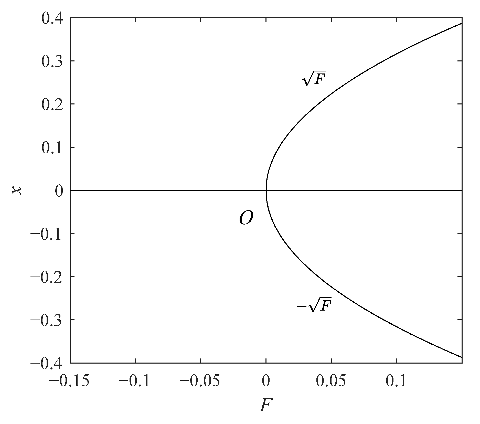
Figure 2.
The bifurcation diagram about Equation (3) for equilibrium .
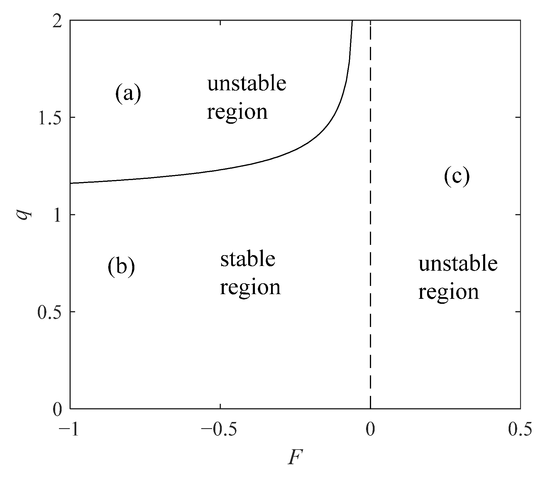
Figure 3.
The bifurcation diagram about Equation (3) for equilibrium .

Figure 4.
Phase diagrams corresponding to the Hopf bifurcation. (a) . (b) The limit cycle near the equilibrium . (c) The limit cycle near the equilibrium .
Figure 4.
Phase diagrams corresponding to the Hopf bifurcation. (a) . (b) The limit cycle near the equilibrium . (c) The limit cycle near the equilibrium .
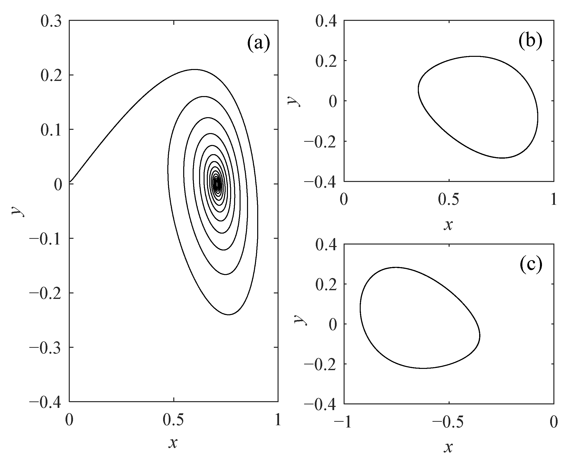
Figure 5.
Phase diagrams corresponding to limit cycles bifurcation for . (a) The limit cycle near the equilibrium . (b) The limit cycle near the equilibrium . (c) The large limit cycle for .
Figure 5.
Phase diagrams corresponding to limit cycles bifurcation for . (a) The limit cycle near the equilibrium . (b) The limit cycle near the equilibrium . (c) The large limit cycle for .
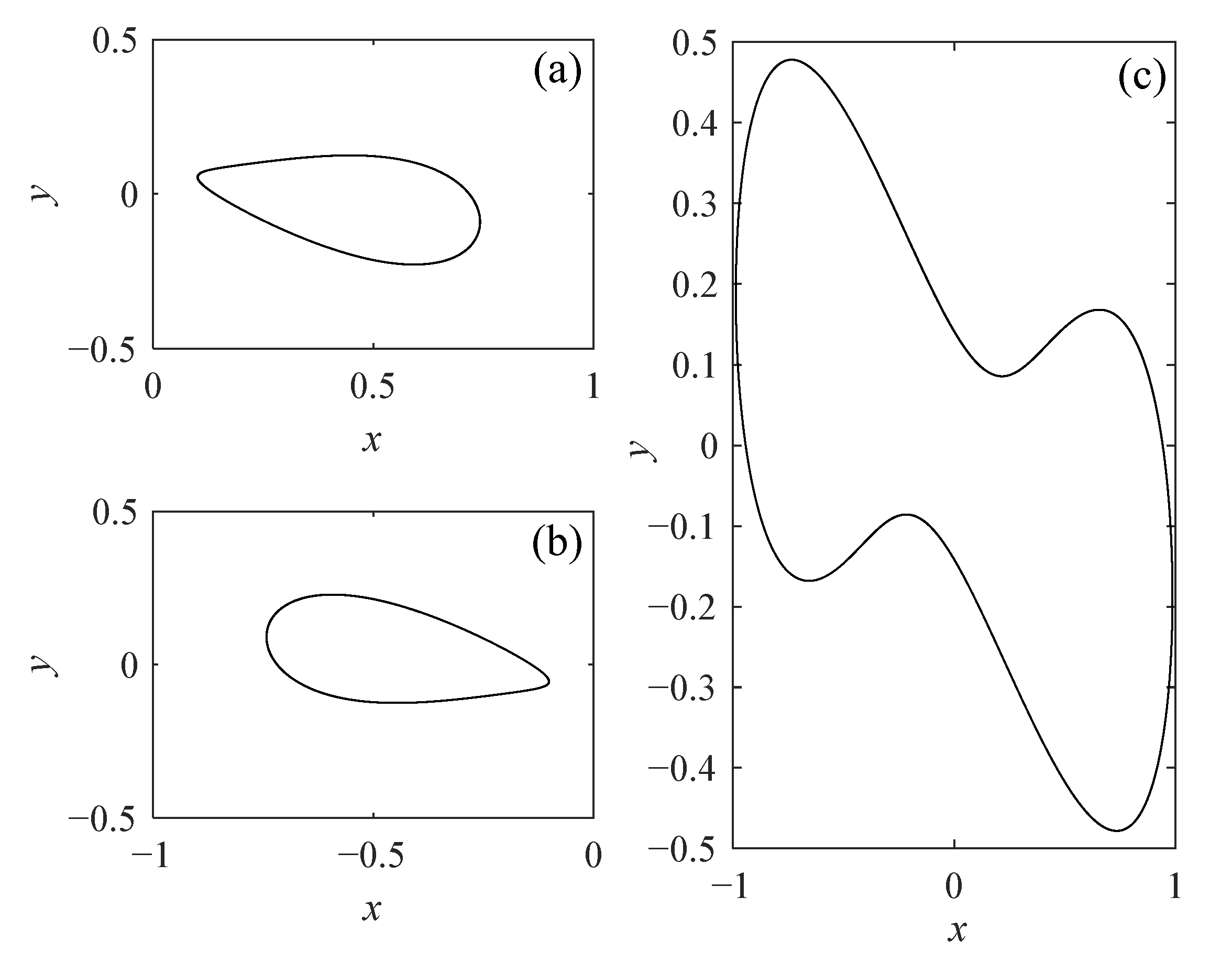
Figure 6.
The bifurcation with respect to the slowly varying parameter and the fractional order of the fast subsystem.
Figure 6.
The bifurcation with respect to the slowly varying parameter and the fractional order of the fast subsystem.
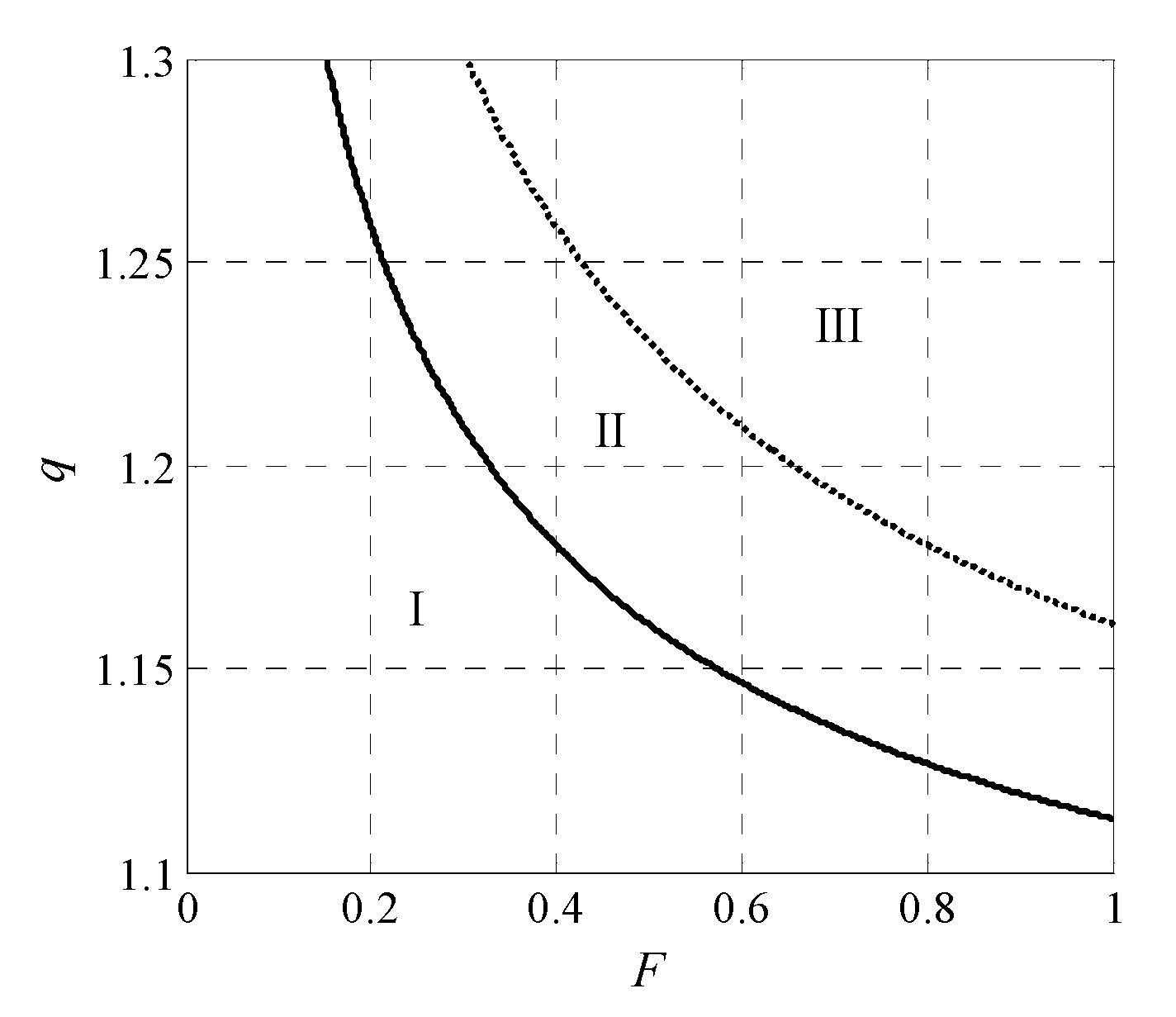
Figure 7.
Bifurcation diagram of Equation (3) for .
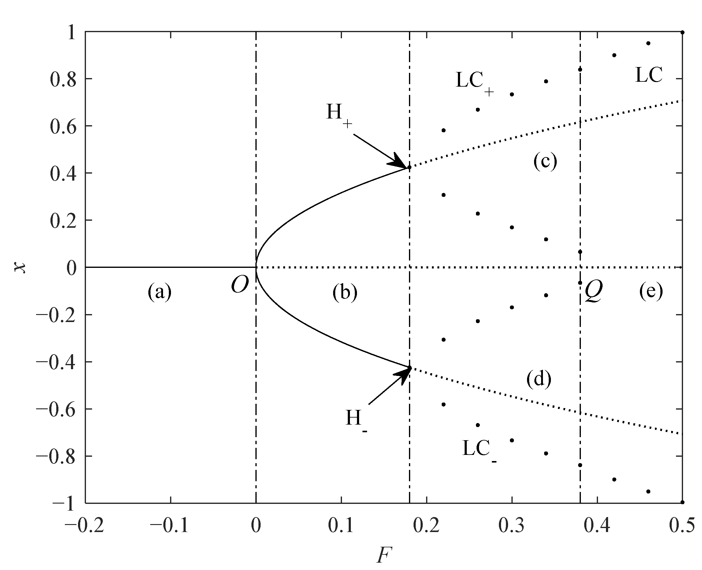
Figure 8.
Cluster oscillation with . (a) Time history diagram. (b) Transition phase diagram for the variable with respect to . (c) Superposition of the transition phase diagram and bifurcation diagram on plane.
Figure 8.
Cluster oscillation with . (a) Time history diagram. (b) Transition phase diagram for the variable with respect to . (c) Superposition of the transition phase diagram and bifurcation diagram on plane.
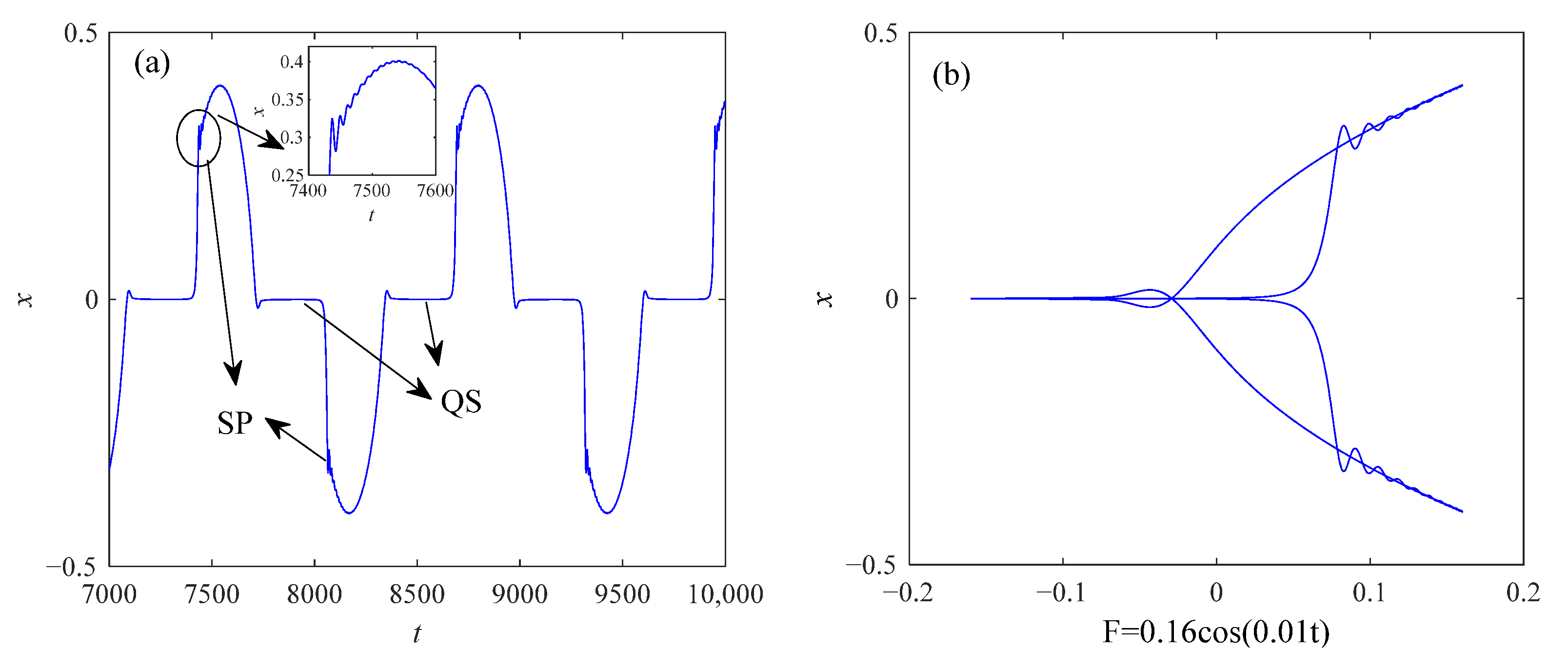
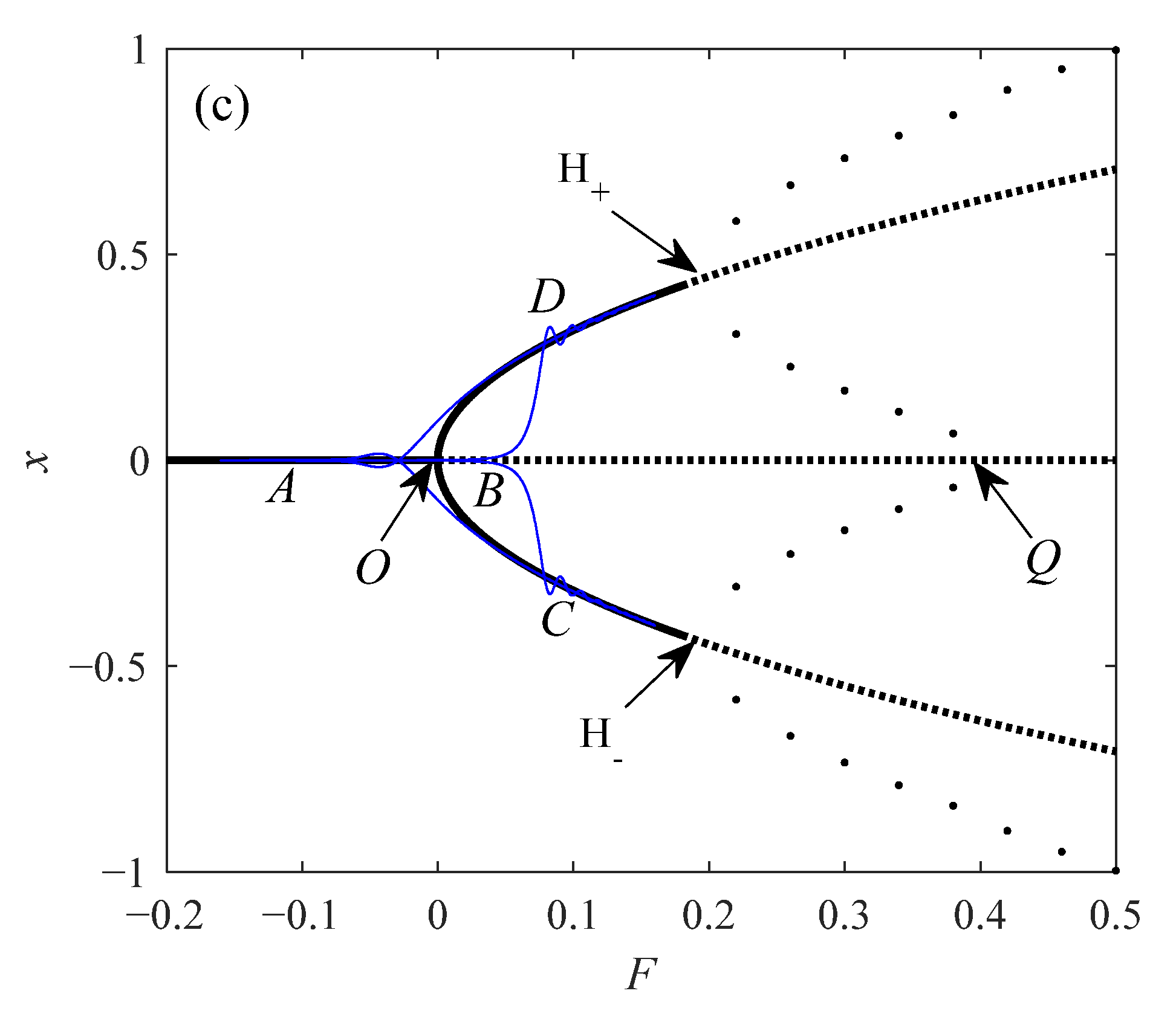
Figure 9.
Cluster oscillation with . (a) Time history diagram. (b1) Superposition of the transition phase diagram and bifurcation diagram on plane for the lower branch. (b2) Superposition of the transition phase diagram and bifurcation diagram on plane for the upper branch.
Figure 9.
Cluster oscillation with . (a) Time history diagram. (b1) Superposition of the transition phase diagram and bifurcation diagram on plane for the lower branch. (b2) Superposition of the transition phase diagram and bifurcation diagram on plane for the upper branch.
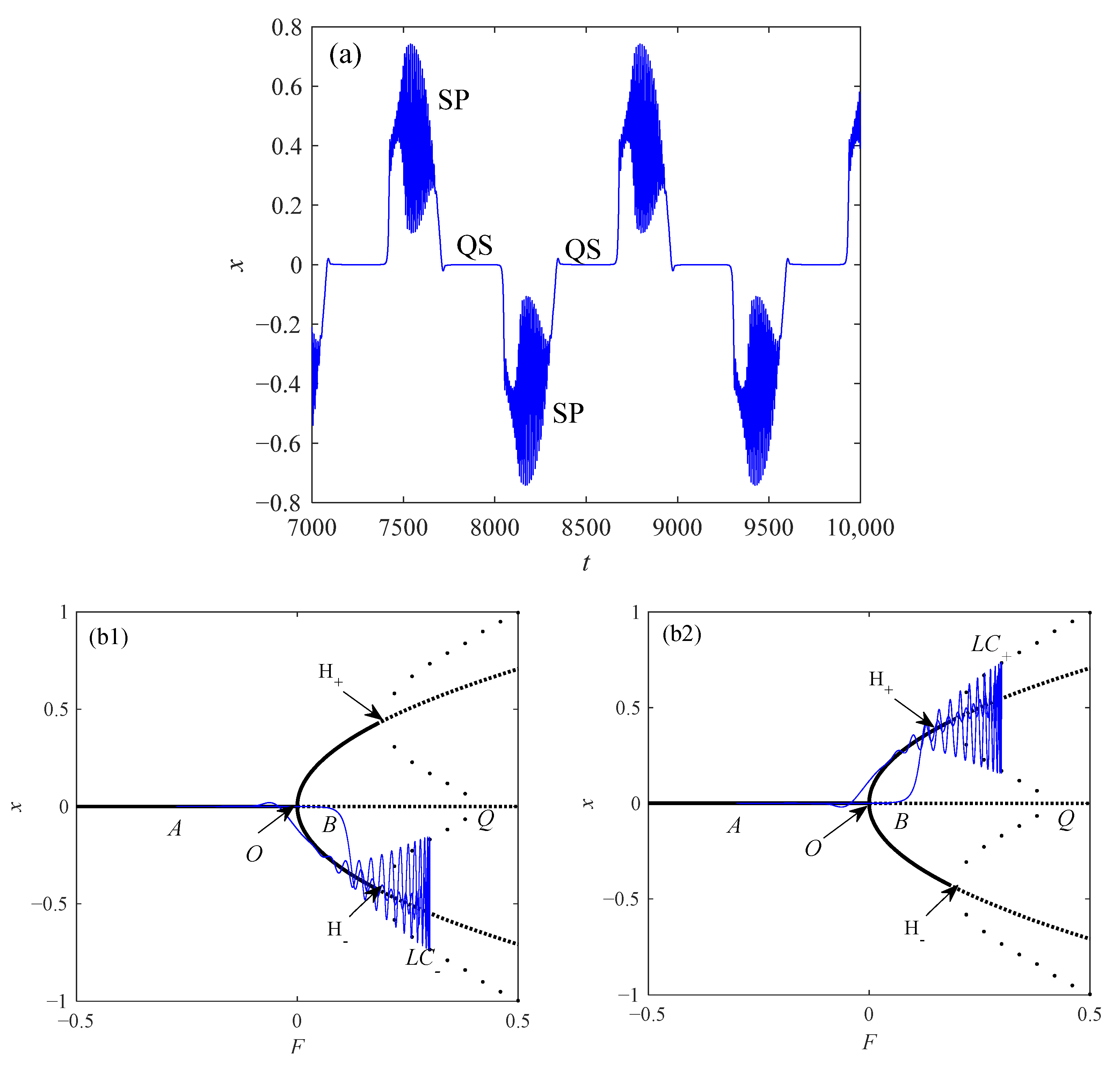
Figure 10.
Cluster oscillation with . (a) Time history diagram. (b) Superposition of the transition phase diagram and bifurcation diagram on plane.
Figure 10.
Cluster oscillation with . (a) Time history diagram. (b) Superposition of the transition phase diagram and bifurcation diagram on plane.

Publisher’s Note: MDPI stays neutral with regard to jurisdictional claims in published maps and institutional affiliations. |
© 2022 by the authors. Licensee MDPI, Basel, Switzerland. This article is an open access article distributed under the terms and conditions of the Creative Commons Attribution (CC BY) license (https://creativecommons.org/licenses/by/4.0/).
Share and Cite
MDPI and ACS Style
Li, X.; Wang, Y.; Shen, Y. Cluster Oscillation of a Fractional-Order Duffing System with Slow Variable Parameter Excitation. Fractal Fract. 2022, 6, 295. https://doi.org/10.3390/fractalfract6060295
AMA Style
Li X, Wang Y, Shen Y. Cluster Oscillation of a Fractional-Order Duffing System with Slow Variable Parameter Excitation. Fractal and Fractional. 2022; 6(6):295. https://doi.org/10.3390/fractalfract6060295
Chicago/Turabian StyleLi, Xianghong, Yanli Wang, and Yongjun Shen. 2022. "Cluster Oscillation of a Fractional-Order Duffing System with Slow Variable Parameter Excitation" Fractal and Fractional 6, no. 6: 295. https://doi.org/10.3390/fractalfract6060295