A Variational Level Set Image Segmentation Method via Fractional Differentiation

Abstract

To solve the issues with conventional level set segmentation algorithms, which are sensitive to the initial contours and less noise-resistant, a segmentation model based on the coupling of texture information and structural information is developed. In this model, a rotation invariant mask produced by fractional-order differentiation is used to first describe the image’s global information. Then, the power function of the energy generalization function is solved by applying factorization theory, and for each pixel of the image, not only its information but also its surrounding pixel information is taken into account and integrated into the energy generalization function via weight scaling. At the same time, the L₂ norm of the fractional-order image and the difference from the fitted image are used to generate the energy generalization function of the model. The final results of this study demonstrate that the proposed model achieved a better segmentation performance than the current active contour models in terms of robustness to Gaussian noise and pretzel noise, as well as the segmentation accuracy and algorithm running time. These results were obtained in synthetic images, real images, and natural images.

1. Introduction

With the continued advancement of science and technology, image processing has become increasingly important. The continuous exploration of images has been extended to various aspects and also applied to a very wide range of fields, among which image segmentation is a very important field in image processing. Images are an essential source of information in people’s daily lives. The fundamental goal of image segmentation is to break an image into many distinct, non-overlapping parts and isolate the area of interest. This creates the framework for further image analysis and comprehension. As a result, one of the main issues with picture segmentation is how to obtain better segmentation results and increase the accuracy and efficiency of segmentation.

Data-driven approaches [1] have had considerable success in semantic segmentation and instance segmentation in recent years with the rapid growth of deep learning, mostly using large-scale labeled datasets for model training. DeepLab v1 [2] combined a deep convolutional neural network and a probabilistic graph model to create an end-to-end network model in 2014, but its low spatial resolution and high storage space requirement prevented it from being widely adopted. Deep learning theory was first applied to segmentation tasks in that year. In order to increase the model optimization capability, the DeepLab v2 [3] void pyramid was proposed. However, this resulted in a decrease in the ability to process image detail blurring. In the same year, the DeepLab v3 [4] improved pyramid structure was proposed. However, this utilized a 1x1 small convolutional kernel, and the output result was poor. In the following year, the DeepLab v3+ [5] encoder–decoder structure was proposed. However, as deep learning technology advanced, some later researchers presented other models for segmentation tasks by fusing deep learning with the traditional king technique. A model that considers the target and background regions, as well as the size of the active contour boundary of the learning process, was proposed by Chen et al. [6] in combination with deep learning. Jie et al. [7] developed an automatic contour refinement (ACR) process to quickly correct incorrect automatic contour segmentation. Although the image segmentation technology based on deep learning has achieved good segmentation results, due to the large amount of data required in the network training process, the results for pixel-level image quality are poor.

Traditional methods [8,9,10,11,12,13,14,15,16] do not require the use of labeled datasets for the initial training of the model, in contrast to deep learning. Traditional techniques work better for the analysis above than deep-learning-based techniques for segmenting images with few labels. Because they can easily extract complex topologies, level-set-based segmentation algorithms [11,12,13,14,15,16] are among the most popular classical methods employed in the field of image segmentation. In order to process the evolution curve and obtain the segmentation results by minimizing the energy generalization, level-set-based approaches for image segmentation typically use edge-based active contour models [11,12,13,14] and region-based active contour models [15,16] that are separated into two groups.

The edge-based active contour model in the level set approach mainly uses the structural information of the image to control the evolution of the curve and detects the boundary of different regions to accurately locate the edge position. However, its disadvantages are also more significant, especially since the detection of weak edges is poor and it is more dependent on the position of the initial curve. In 1988, Kass et al. first proposed the active contour model, called the snake model [17], which has the advantage of being able to obtain closed target boundaries. However, because the model only refers to the edge information of the image, it has the problem of not converging correctly to the edge of the target region. Since this model only refers to the edge information, it has problems such as not converging correctly to the depressed part of the target region edge. To address the above problems, Caselles et al. [18] proposed the geodesic active contour (GAC) model, which uses the image gradient information to construct an edge stop function so that the evolution curve finally stops at the target boundary to achieve the segmentation process. Since this model only uses the image gradient information, it cannot obtain good segmentation results for noisy images, low-contrast images, and weak-edged images.

The active-region-based contour model in the level set approach mainly uses the region information in the image to evolve the curve and can segment the internal boundaries as well as the weaker edges better. For example, the CV model [19] mainly assumes that the grayscale within the foreground and background regions is always constant, and it has the disadvantage that it does not apply to images with an uneven grayscale. To address these problems, Li et al. [20] proposed the region-scalable fitting (RSF) model by using local image information, approximating the grayscale on both sides of the contour with two fitting functions, and deriving the curve evolution equation for energy minimization using the regularized variational level set formulation. This model can segment grayscale inhomogeneous images with high accuracy. Zhang et al. [21] proposed a local image fitting (LIF) energy function model based on minimizing the difference between the fitted image and the original image to improve the segmentation efficiency of the algorithm. Ho Sub Lee et al. [22] used the texture information of the image and proposed an image segmentation method based on a spatial color histogram; the proposed method has a fast computing speed and good segmentation quality.

Although image segmentation models based on the level set method have achieved excellent results, the method is more sensitive to the position selection and noise of the initialized contour, and it is easy to fall into local optimality. In recent years, researchers have explored these problems more extensively for the active contour model, mainly by incorporating texture information or structural information into the active contour model for segmentation experiments.

More results have been achieved for segmentation using the texture information of images. Min et al. [23] proposed a color texture segmentation method that focuses on combining intensity and texture terms into an energy function. Liu et al. [24] proposed a texture image segmentation method based on local Gaussian distribution fitting and local self-similarity, which has low time complexity. Subuh et al. [25] proposed a hybrid energy-based image feature structure algorithm that evolves the contour curve toward the desired texture boundary. Yuan et al. [26] proposed a texture image segmentation method that uses factorization theory to analyze the components of each feature vector and assign a pixel to the region with the largest weight. Gao et al. [27] proposed a natural image segmentation method based on texture features and factorization that uses a local spectral histogram to represent texture features, which provides a new way to effectively use different features in the active contour method. Gao et al. [28] proposed a texture image segmentation model based on statistical active contours.

For segmentation using the structural information of images, integer-order gradient-based active contour models have achieved better results, but such models are less robust to noise while improving the visual quality of images. Compared with integer-order gradients, fractional-order gradients can better characterize images and have been successfully applied to several research areas such as image denoising [29,30], image restoration [31,32], and image fusion [33,34]. Chen et al. [35] introduced fractional-order Gaussian kernel functions into the data fidelity term of their model and used the local region grayscale information of the controllable range to level. Zhang et al. [36] proposed a method combining fractional-order differentiation and locally fitted energy, mainly by combining the fitted image and fractional-order differentiation to obtain rich image detail information for constructing energy floods. Li et al. [37] proposed an active contour model using a Gaussian kernel function and fractional-order differentiation to design the data in terms of energy floods; based on the order of the fractional-order differentiation, the nature of the pixel can be modified accordingly.

In this paper, a fractional-order differential segmentation model based on the local information of images is proposed to address the problems of the classical model in the image segmentation process that is sensitive to the selection of the initial contour position and noise. The main contributions are as follows:

(1) An image segmentation model based on fractional-order differentiation is proposed, which mainly applies fractional-order differentiation to the original image in order to make it calculate with the fitted image, using the idea that the fractional order is better than the integer order for constructing a new energy generalization to overcome the problem of poor global of the original image.

(2) For the initial contour robustness problem, factorization theory is used to solve the weight function, which improves the classical model’s uncertainty in choosing the initial contour position of the evolution curve and overcomes the problem of being sensitive to noise. Meanwhile, the local spectral histogram is further analyzed as the texture feature of the original image in the process of performing the solution.

(3) Segmentation experiments were carried out using images rich in structural information and images rich in texture information, and the segmentation results of the model were compared with the state-of-the-art model in the experiments. The experimental results show that the proposed model has a high segmentation accuracy, while the segmentation time of the model in this paper is shorter on the premise that the target boundary can be extracted accurately.

The rest of this paper is organized as follows: related work is presented in Section 2. The proposed image segmentation model based on fractional-order differentiation is described in Section 3. The experimental results are presented in Section 4, and the conclusions are drawn in Section 5.

2. Related Work

2.1. The LIF Model

The LIF model [21] takes the local fitting image (LFI) as the basis, uses the Gaussian kernel as a measure of the local pixel distance, and finally uses the local mean for image segmentation. For a point in the image region, its local image fitting function is defined as follows:

$$I^{\mathrm{LFI}}=m_1{H}_{\epsilon }(\varphi )+m_2(1-H_{\epsilon }(\varphi ))$$

(1)

where $I:\mathsf{\Omega }\subset R^2\to R$ input image, $\varphi$ is the embedding function of the evolutionary curve C, $H_{\epsilon }(\varphi )$ is the regularized Heaviside function, and $m_1$ and $m_2$ are the locally weighted average grayscales of the image:

$$m_1=mean(I(x)\in (\{x\in \mathsf{\Omega }|\varphi (x)<0\}\cap W_k(x)))$$

(2)

$$m_2=mean(I(x)\in (\{x\in \mathsf{\Omega }|\varphi (x)>0\}\cap W_k(x)))$$

(3)

where $W_k\left(x\right)$ denotes a Gaussian window of size $k$.

The energy generalization function of the LIF model is defined as:

$${\mathrm{E}}^{\mathrm{LIF}}(\varphi )=\frac{1}{2}{\displaystyle {\int }_{\mathsf{\Omega }}{(I(x)-I^{\mathrm{LFI}}(x))}^2}\mathrm{d}x$$

(4)

The gradient descent flow of the level set function $\varphi$ can be obtained using the variational principle:

$$\frac{\partial \varphi }{\partial t}={\delta }_{\epsilon }(\varphi (x))(I(x)-I^{\mathrm{LFI}}(x))(m_1-m_2)$$

(5)

where ${\delta }_{\epsilon }(\varphi )$ is the regularized Dirac function.

2.2. Texture Features

For texture feature selection, the factorization-based active contour model proposed by Gao et al. [27] was utilized. This method mainly uses the local spectral histogram as the texture feature and establishes a new energy functional based on matrix decomposition theory:

$$\mathrm{E}(\varphi ,R)=\mu {\mathrm{E}}_{data}(\varphi ,R)+\nu {\mathrm{E}}_{regularization}(\varphi )$$

(6)

$${\mathrm{E}}_{data}(\varphi ,R)=-{\displaystyle {\int }_{\mathsf{\Omega }}(H_{\epsilon }(\varphi ){\omega }_0(x,R)+(1-H_{\epsilon }(\varphi )){\omega }_b(x,R))\mathrm{d}x}$$

(7)

$${\mathrm{E}}_{regularization}(\varphi )=\frac{1}{2}{\displaystyle {\int }_{\mathsf{\Omega }}{(\left|\nabla \varphi (x)\right|-1)}^2\mathrm{d}x}$$

(8)

where ${\mathrm{E}}_{data}(\varphi ,R)$ is the data term, ${\mathrm{E}}_{regularization}(\varphi )$ is the regular term, $\mu$ and $\nu$ are two constants, used to balance the proportion of the total energy in its corresponding term, ${\omega }_0$ and ${\omega }_b$ denote the combined weights of all pixels in the image, and $\nabla \varphi$ denotes the gradient of the level set function.

2.3. Structural Features

Fractional calculus is a natural generalization of integer calculus. Fractional differential operators can greatly improve the structural features of images in the process of image enhancement. For an image, $I\left(x,y\right)$ is the gray value at pixel $\left(x,y\right)$, and the numerical expression of its fractional differential can be expressed as:

$$\frac{{\partial }^{v}I\left(x,y\right)}{\partial x^v}\approx I\left(x,y\right)+\left(-v\right)I\left(x-1,y\right)+\frac{\left(-v\right)\left(-v+1\right)}{2!}I\left(x-2,y\right)+\cdots +\frac{\mathsf{\Gamma }\left(-v+m-1\right)}{\left(m-1\right)!\mathsf{\Gamma }\left(-v\right)}I\left(x-m+1,y\right)$$

(9)

$$\frac{{\partial }^{v}I\left(x,y\right)}{\partial y^v}\approx I\left(x,y\right)+\left(-v\right)I\left(x,y-1\right)+\frac{\left(-v\right)\left(-v+1\right)}{2!}I\left(x,y-2\right)+\cdots +\frac{\mathsf{\Gamma }\left(-v+m-1\right)}{\left(m-1\right)!\mathsf{\Gamma }\left(-v\right)}I\left(x,y-m+1\right)$$

(10)

where

$$\{\begin{array}{l}{\omega }_0=1\begin{array}{cccc}\begin{array}{ccc}\begin{array}{ccc}\begin{array}{cc}\begin{array}{cc}& \end{array}& \end{array}& & \end{array}& & \end{array}& & & \end{array}\hfill \\ {\omega }_1=-v\begin{array}{cccc}\begin{array}{ccc}\begin{array}{cc}& \end{array}& & \begin{array}{cc}\begin{array}{cc}& \end{array}& \end{array}\end{array}& & & \end{array}\hfill \\ {\omega }_2=\frac{\left(-v\right)\left(-v+1\right)}{2!}\begin{array}{cccc}\begin{array}{cc}\begin{array}{cc}& \end{array}& \end{array}& & & \end{array}\hfill \\ {\omega }_3=\frac{\left(-v\right)\left(-v+1\right)\left(-v+2\right)}{3!}\begin{array}{cc}\begin{array}{cc}\begin{array}{cc}& \end{array}& \end{array}& \end{array}\hfill \\ {\omega }_4=\frac{\left(-v\right)\left(-v+1\right)\left(-v+2\right)\left(-v+3\right)}{4!}\begin{array}{cc}& \end{array}\hfill \end{array}$$

(11)

3. The Proposed Model

In this paper, we propose a new image segmentation model based on fractional-order differentiation (NFD-LIF) to address the problems of the classical LIF model in the selection of the initial contour position of the curve and noise sensitivity, mainly by combining the classical LIF model with the theory of factorization to construct a new energy generalization and, at the same time, using fractional-order differentiation to represent the image.

3.1. Energy Functional of the NFD-LIF Model

The local data fitting terms for the energy functional of the NFD-LIF model are

$$I^{\mathrm{W}-\mathrm{LFI}}={\kappa }_1{H}_{\epsilon }(\varphi )+{\kappa }_2(1-H_{\epsilon }(\varphi ))$$

(12)

where $H_{\epsilon }(\varphi )$ is the smooth Heaviside function, the ${\kappa }_1$ and ${\kappa }_2$ denote the weights of the target and background regions in $I$. For ${\kappa }_1$ and ${\kappa }_2$, the solution procedure is detailed in [27].

The new energy functional is constructed using the data fitting term, while the original image is characterized by the information using fractional-order differentiation, as follows:

$${\mathrm{E}}^{\mathrm{NFD}-\mathrm{LIF}}=\frac{1}{2}{\displaystyle {\int }_{\mathsf{\Omega }}{{(\mathrm{D}}^{\nu }I\left(x\right)-I^{\mathrm{W}-\mathrm{LFI}})}^2}\mathrm{d}x,x\in \mathsf{\Omega }$$

(13)

where $I\left(x\right)$ is the original image, $\mathsf{\Omega }$ is the image domain, and ${\mathrm{D}}^{\nu }$ is the fractional-order differential operator that maps the original image to the fractional-order domain, and $I^{\mathrm{W}-\mathrm{LFI}}$ is the fitted image. The LIF model is a special case of the NFD-LIF model at this point when ${\mathrm{D}}^{\nu }=\mathrm{E}$ ($\mathrm{E}$ is an identical transformation) and ${\kappa }_i=m_i(i=1,2)$ in $I^{\mathrm{W}-\mathrm{LFI}}$. A comparative analysis with the LIF model was also carried out during the experimental validation process, as detailed in Section 4.

For a better representation of the features of the image, the input image is convolved in eight directions using a fractional-order mask operator [38], and the convolution results obtained from the eight directions are integrated to obtain a fit of the overall input image, i.e.,

$${\mathrm{D}}^{v}I=\frac{I\ast I_x^{+}+I\ast I_x^{-}+I\ast I_y^{+}+I\ast I_y^{-}+I\ast I_{\mathrm{LDD}}+I\ast I_{\mathrm{RUD}}+I\ast I_{\mathrm{RDD}}+I\ast I_{\mathrm{LUD}}}{8\cdot ({\displaystyle \sum _{i=0}^4{\omega }_i})}$$

(14)

The eight selected directions are as follows: the $x$ positive direction, and the $x$ negative direction; the $y$ positive direction, and the $y$ negative direction; the lower left diagonal, upper right diagonal, upper left diagonal, and lower right diagonal (Figure 1).

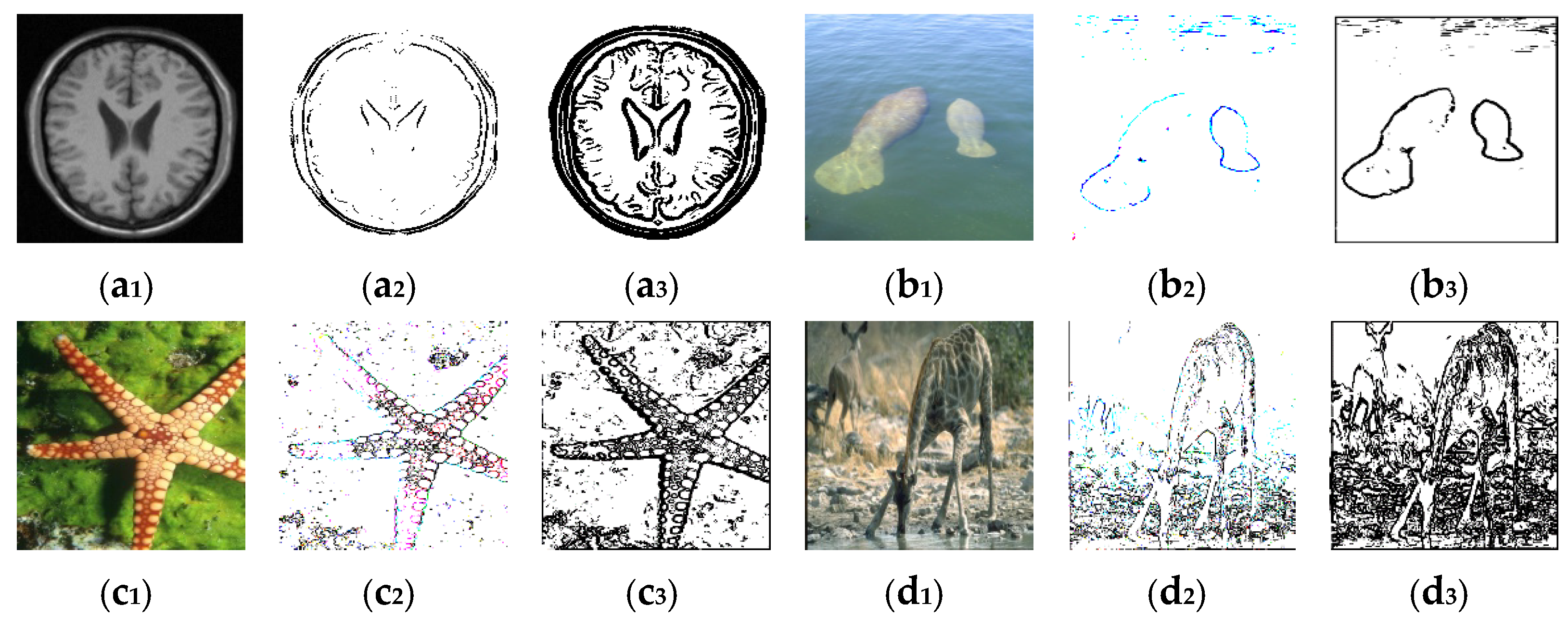
The following is the fractional feature verification of the model, four images were selected from the Berkely Segmentation Dataset BSDS500 [39]. The gradient maps of the original images, the gradient maps of the integer-order images, and the gradient maps of the fractional-order images are presented in Figure 2. (a₁) is a brain magnetic resonance imaging(MRI) image. (a₂) is the corresponding integer-order gradient map. It can be seen from (a₂) that it is better for the large edge contour of the brain but not detailed enough for a detailed description. (a₃) is the corresponding fractional-order gradient map. It is clearer in terms of the internal details and can roughly reflect the specific information of (a₁). (b₁) is an image of marine organisms. (b₂) is the corresponding integer-order gradient map. From (b₂), it can be seen that the edge contours are better for the small fish, but the edge contours of the large fish are not clearly defined. (b₃) is the corresponding fractional-order gradient map. Relative to (b₂), the edge contours of the large fish are clearer and can roughly reflect the specific information of (b₁). (c₁) is an image of a starfish. (c₂) is the corresponding integer-order gradient map. From (c₂), it can be seen that for the five antennae of the starfish, the edge contours of three antennae are better, and the edge contours of the other two antennae are not clearly defined. (c₃) is the corresponding fractional-order gradient map. Compared with (c₂), the edge contours of the five antennae of the starfish are clearer and can reflect the specific information of (c₁). (d₁) is an image of an animal. (d₂) is the corresponding integer-order gradient map. From (d₂), it can be seen that the edges of the big deer are more clearly carved out, but those of the small deer are more blurred, and the information of the deer can hardly be seen. (d₃) is the corresponding fractional-order gradient map. Compared with (d₂), the edges of both the big deer and the small deer are more clearly outlined and can reflect the specific information of (d₁). From the above analysis, it can be seen that the fractional-order gradient has significant advantages in extracting the detailed information of the images compared with the integer-order gradient, so the NFD-LIF model uses the fractional order to represent the information of the images.

For the experiments performed in Figure 2, the theoretical analysis in [40] explains the superiority of fractional-order differentiation over integer-order differentiation. While integer-order differentiation greatly enhances noise while greatly attenuating weak edges and regions of texture detail, fractional-order differentiation has the property of simultaneously enhancing high-frequency signals and preserving low- and mid-frequency signals, i.e., weak edges and texture detail of the image can be preserved during image pre-processing [41].

3.2. Energy Functional Solution

The generalized function mentioned in Equation (13) needs to be obtained by minimizing the difference between the fitted image and the fractional-order image by differentiating the level set function $\varphi$, i.e., $\stackrel{\sim }{\varphi }=\varphi +{\epsilon }_1\eta$, and fixing ${\kappa }_1$ and ${\kappa }_2$, differentiating it for $\varphi$. When ${\epsilon }_1\to 0$, we have:

$$\begin{gathered} \frac{\delta {\mathrm{E}}^{\mathrm{NFD}-\mathrm{LIF}}}{\delta \varphi }=\underset{{\epsilon }_1\to 0}{\lim }\frac{\mathrm{d}}{\mathrm{d}{\epsilon }_1}(\frac{1}{2}{\displaystyle {\int }_{\mathsf{\Omega }}{({\mathrm{D}}^{\nu }I-{\kappa }_1{H}_{\epsilon }(\stackrel{\sim }{\varphi })-{\kappa }_2(1-H_{\epsilon }(\stackrel{\sim }{\varphi })))}^2\mathrm{d}x} \\ =\underset{{\epsilon }_1\to 0}{\lim }(-{\displaystyle {\int }_{\mathsf{\Omega }}({\mathrm{D}}^{\nu }I-{\kappa }_1{H}_{\epsilon }(\stackrel{\sim }{\varphi })-{\kappa }_2{H}_{\epsilon }(\stackrel{\sim }{\varphi }))({\kappa }_1-{\kappa }_2){\delta }_{\epsilon }(\stackrel{\sim }{\varphi })\eta \mathrm{d}x}) \\ =-{\displaystyle {\int }_{\mathsf{\Omega }}({\mathrm{D}}^{\nu }I-{\kappa }_1{H}_{\epsilon }(\varphi )-{\kappa }_2{H}_{\epsilon }(\varphi ))({\kappa }_1-{\kappa }_2){\delta }_{\epsilon }(\varphi )\eta \mathrm{d}x} \end{gathered}$$

(15)

According to the variational principle, the gradient descent flow of Equation (13) is obtained as:

$$\frac{\partial \varphi }{\partial t}=({\mathrm{D}}^{\nu }I-{\kappa }_1{H}_{\epsilon }(\varphi )-{\kappa }_2{H}_{\epsilon }(\varphi ))({\kappa }_1-{\kappa }_2){\delta }_{\epsilon }(\varphi )$$

(16)

3.3. Regular Term Constraints

To make the curve evolve in such a way that the level set function is sufficiently sensitive past the zero point while remaining smooth in regions far from the zero level set, the canonical term from [16] is adopted:

$${\phi }_R=\tanh (\eta {\phi }^{n+1})$$

(17)

$${\phi }_L(x)=mean({\phi }_R(y)|y\in {\mathsf{\Omega }}_x)$$

(18)

where $\eta$ is a fixed constant, for $\eta$, we use the parameter proposed in document [16] $\eta =7$. The purpose of formula (17) is to improve the slope of the level set function in the zero-crossing region and suppress the slope of the two high points. $\phi (x)$ is the intensity of the horizontal setpoint on $x$, ${\mathsf{\Omega }}_x$ represents a small area of size $(2k+1)\times (2k+1)$, and $mean$ represents the average intensity value in the calculation window.

3.4. Validation of the NFD-LIF Model

The following experiments were conducted on grayscale images, natural images, and noisy images with different types of noise as well as different levels of noise for the NFD-LIF model.

3.4.1. Verifying the Robustness of NFD-LIF Model to the Initial Contours

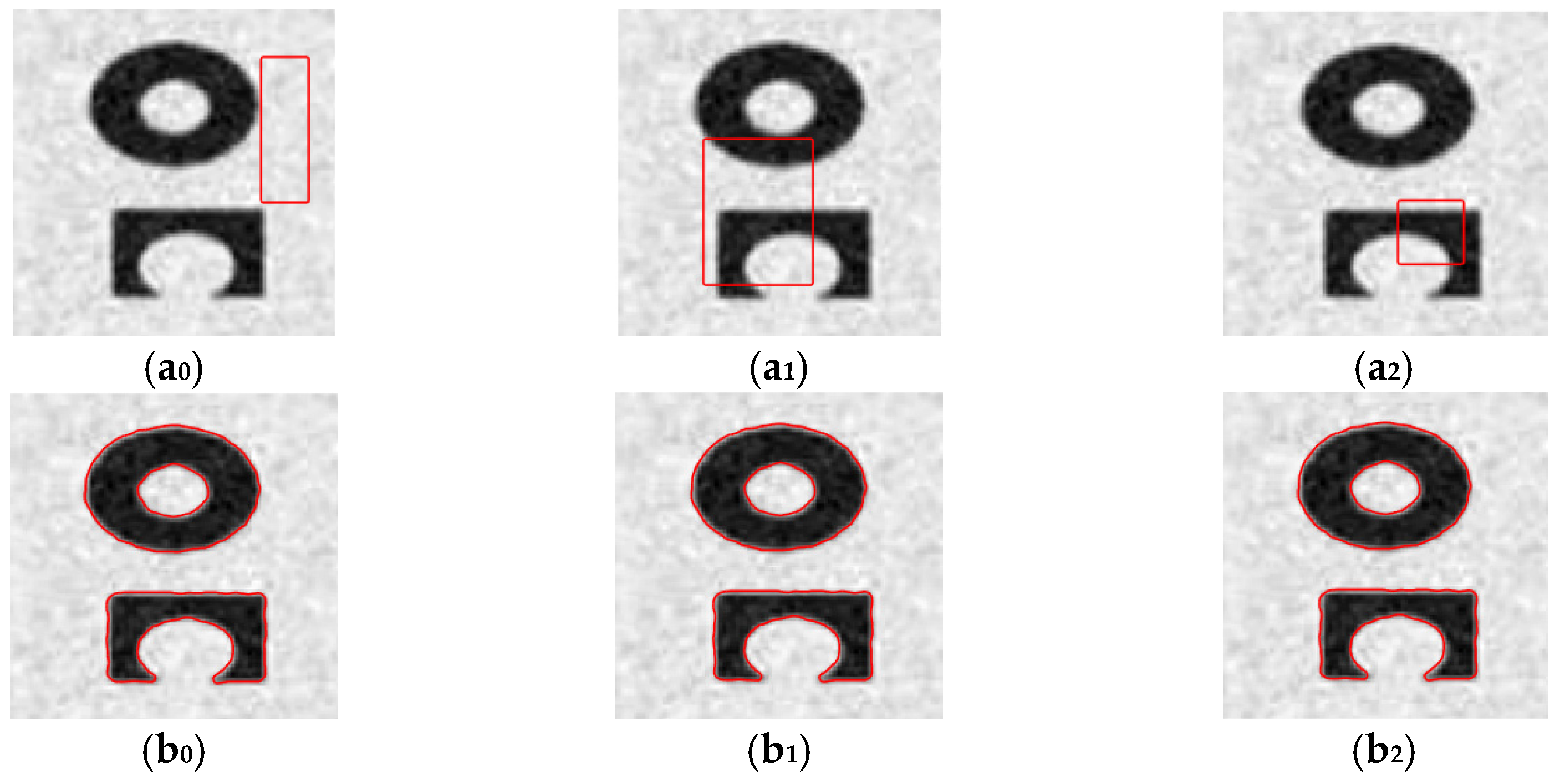
For the synthetic image, three different initial contours were selected for the experiment. The first row in Figure 3 shows the images containing different initial contours, where the red rectangles represent the initial contours, and the second row shows the segmentation results of the NFD-LIF model.

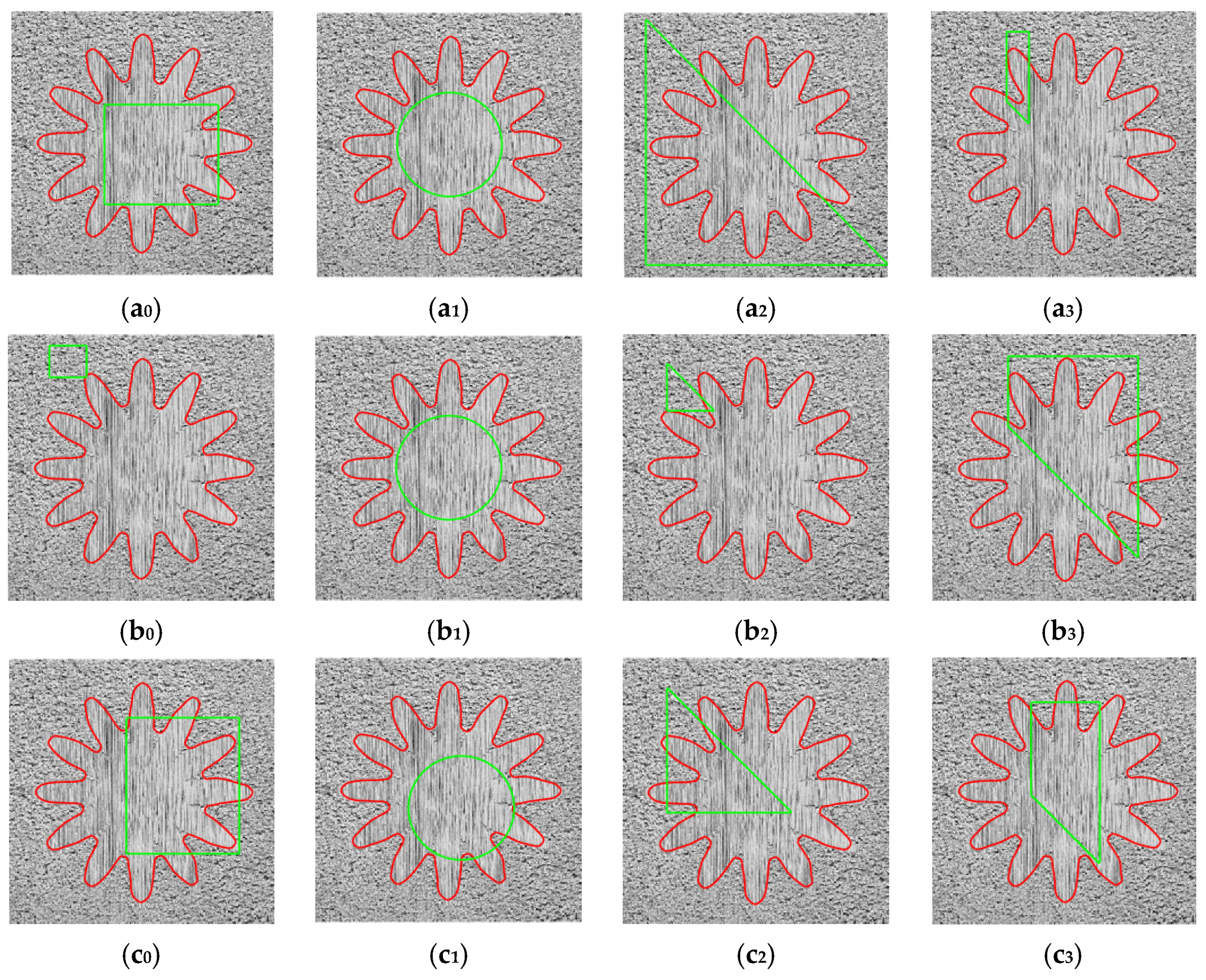
From Figure 3, we can find that (a₀) is the initial contour without a target, (a₁) is the initial contour with two targets, and (a₂) is the initial contour with one target. (b₀), (b₁), and (b₂) are the results of the NFD-LIF model segmentation corresponding to (a₀), (a₁), and (a₂), respectively. The NFD-LIF model accurately segmented the initial contour when it contained one target, when it contained two targets, and when it did not contain targets. The initial verification of the robustness of the initial contour was tested on the texture image by setting different positions of the initial contour, and the segmentation results are shown in Figure 4.

From Figure 4, in (a₀,b₀,c₀), (a₁,b₁,c₁), (a₂,b₂,c₂), and (a₃,b₃,c₃) the green represents the initial contour, and the red color indicates the segmentation result. As shown in all of the segmentation results, the NFD-LIF model segmented the texture image accurately regardless of whether the shape of the initial contour was a rectangle, circle, triangle, or trapezoid, or whether it contained the segmentation target.

3.4.2. Verifying the Robustness of NFD-LIF Model to Noise

To further analyze the validity of the model, experimental validation was performed from two different perspectives.

(1) Subjective assessment analysis

We initially set the contour as a circle and then selected the real image and added Gaussian noise. Then, we also added pretzel noise, respectively, to the image. The segmentation results are shown in Figure 5. The first row shows the noise-added images, and the second row shows the segmented images.

Figure 5 shows the results of adding different levels of Gaussian noise to the image (a₀) and (b₀), and the results of adding different levels of pretzel noise to the image (c₀) and (d₀). The size and shape of the coin can be seen in (a₀), (b₀), and (c₀) from the original image (a₀), but the foreground and background of (d₀) are almost blended into one, and the segmentation target is blurred. We can see from the segmentation results in (a₁) to (d₁) that the clearer image and the image with an almost integrated background both have better segmentation results. The segmentation results in Figure 5 demonstrate that the NFD-LIF model achieved real image segmentation with varying levels of noise, as well as having good robustness to noise.

Six images from the Berkely Segmentation Dataset BSDS500 [39] were chosen to test the experimental feasibility of natural images, and the segmentation results are shown in Figure 6.

According to Figure 6, the NFD-LIF model segmented natural images in different scenes as well as noise-added natural images in different scenes, proving the feasibility and effectiveness of the NFD-LIF model for natural image segmentation.

(2) Objective assessment analysis

Figure 6 above underwent the following objective examination utilizing the following four indices in order to properly analyze the experimental results, see

Table 1. Objective Assessment.

Test Image	DSC	Precision	Recall	JSC
Figure 6(b0)	0.9804	0.9701	0.9908	0.9615
Figure 6(b1)	0.9850	0.9721	0.9982	0.9704
Figure 6(b2)	0.9916	0.9870	0.9963	0.9834
Figure 6(b3)	0.9787	0.9856	0.9718	0.9582
Figure 6(b4)	0.9803	0.9636	0.9978	0.9614
Figure 6(b5)	0.9775	0.9890	0.9662	0.9559

for objective evaluation results.

The Jaccard’s index (JSC) rate [42] is the area of overlap between the predicted segmentation and the label divided by the joint area between the predicted segmentation and the label (intersection of the two/merger of the two), which is given by:

$$\mathrm{JSC}=\frac{\left|{\mathrm{G}}_{\mathrm{S}}\cap {\mathrm{G}}_{\mathrm{G}\mathrm{T}}\right|}{\left|{\mathrm{G}}_{\mathrm{S}}\cup {\mathrm{G}}_{\mathrm{G}\mathrm{T}}\right|}$$

(19)

The dice similarity coefficient (DSC) rate [43] is an ensemble similarity measure function that is commonly used to calculate the similarity of two samples. The formula is as follows:

$$\mathrm{D}\mathrm{S}\mathrm{C}=\frac{2\left|{\mathrm{G}}_{\mathrm{S}}\cap {\mathrm{G}}_{\mathrm{G}\mathrm{T}}\right|}{\left|{\mathrm{G}}_{\mathrm{S}}\right|+\left|{\mathrm{G}}_{\mathrm{G}\mathrm{T}}\right|}$$

(20)

Precision [44] is the probability that a pixel in a segmentation result is correctly segmented. The formula is as follows:

$$\mathrm{Precision}=\frac{\mathrm{T}\mathrm{P}}{\mathrm{T}\mathrm{P}+\mathrm{F}\mathrm{P}}\times 100\%$$

(21)

Recall [44] also known as check-all rate, expresses the meaning of the probability that a pixel in a ground truth (GT) image is correctly segmented. The formula is as follows:

$$\mathrm{Recall}=\frac{\mathrm{T}\mathrm{P}}{\mathrm{T}\mathrm{P}+\mathrm{F}\mathrm{N}}\times 100\%$$

(22)

Among the above four commonly used objective evaluation metrics, ${\mathrm{G}}_{\mathrm{S}}$ denotes the image after algorithm segmentation, ${\mathrm{G}}_{\mathrm{G}\mathrm{T}}$ denotes the GT image, $|\cdot |$ denotes the number of pixels in the region, $\mathrm{T}\mathrm{P}$ denotes the true example, $\mathrm{F}\mathrm{P}$ denotes the false positive example, and $\mathrm{F}\mathrm{N}$ denotes the false negative example.

Table 1 shows the objective evaluation results of the NFD-LIF model for the natural image segmentation results, in which the four objective indicators take values in the range of [0,1], where the closer the objective evaluation value is to 1, the better the segmentation effect; the closer it is to 0, the worse the segmentation effect. From Table 1, we can find that for the DSC evaluation index, the segmentation error rate had a range of 0.84% to 2.25%. For the precision index, the segmentation error rate had a range of 1.1% to 3.74%. For the recall evaluation index, the segmentation error rate had a range of 0.16% to 3.38%. For the JSC index, the segmentation error rate had a range of 1.66% to 3.76%. The segmentation error rate for the JSC index ranged from 1.66% to 4.41%, thus further validating the effectiveness of the NFD-LIF model.

4. Comparative Experimental Results and Analysis

The color images selected for the experiments in this paper were from the Berkely Segmentation Dataset BSDS500 [39], all experiments were performed using MATLAB R2018b, and the internal environment was a Windows 10 (64 bit)-Intel(R) Core (TM) i7-11800H (Lenovo Co. LTD, Beijing, China) running on a computer with a 2.30 GHz CPU and 16GB RAM.

4.1. Segmentation Results of the Model for Structurally Information-Rich Images

To verify the robustness of the NFD-LIF model to noise, the synthetic images with added Gaussian noise were compared. The LBF model, LIC model, model from [16], model from [27], and NFD-LIF model were compared for the experiments, and the segmentation results are shown in Figure 7. Column 1 indicates the Gaussian noise images with a mean of 0 and variances of 0.01, 0.05, 0.09, and 0.13. Columns 2 to 5 show the segmentation results of the LIC model, LBF model, model from [16], and model from [27], respectively, and column 6 shows the segmentation results of the NFD-LIF model. To demonstrate the segmentation performance and efficiency of the various models, the comparison results of the number of iterations and running time are shown in

Table 2. Running Time and Number of Iterations of the Active Contour Model with Different Gaussian Noise Levels.

Model	0.01		0.05		0.09		0.13
	Time (s)	Iterations	Time (s)	Iterations	Time (s)	Iterations	Time (s)	Iterations
LIC	2.763	50	4.103	70	5.393	100	7.792	150
LBF	3.107	70	3.731	90	5.122	120	8.788	200
Model from [16]	0.934	50	1.142	70	1.417	100	1.782	150
Model from [27]	4.228	60	5.134	60	6.184	100	6.201	100
NFD-LIF	2.580	17	2.924	25	3.165	30	3.435	30

.

In Figure 7, (a₀), (b₀), (c₀), and (d₀) show the results of adding different levels of Gaussian noise to the image. Analyzing the unsegmented images (a₀,b₀,c₀,d₀), the size, as well as the shape of the segmented target, can be observed in (a₀), but the segmented targets in (b₀), (c₀), and (d₀) are gradually blurred. The LIC model extracted the target boundary in (a₁) when the foreground and background were clear, but the extracted boundary was not smooth and could not be accurately segmented. As the noise level increased, the damage to the segmented target increased in turn, and the smoothness of the target boundary became increasingly worse. The LBF model extracted the target boundary in (a₂) when the foreground and background were clear, although the extracted boundary was not smooth. As the noise corruption became increasingly severe, as seen in (b₂), (c₂), and (d₂), the target boundary could not be extracted accurately. The model from [16] extracted the smooth target curve from the background in (a₃) when the foreground and background were clear. However, as the noise corruption became increasingly serious, the target boundary extraction became increasingly worse, and even the target boundary (d₃) could not be extracted. With the model from [27], the target boundary was able to be extracted when the foreground and background of (a₄) were clear, and the extracted boundary was smooth. From (b₄), (c₄), and (d₄), it can be seen that the target boundary extraction worsened. The NFD-LIF model extracted the target boundary not only with a clear foreground and background in the case of (a₁) but also with a complex background, and the extracted boundary was smooth. According to the segmentation results, the LIC model, LBF model, model from [16], and model from [27] were more sensitive to Gaussian noise, which led to a decrease in the segmentation accuracy or even an inability to perform complete segmentation. Meanwhile, the NFD-LIF model obtained better segmentation results for both clearer images and blurred images and had a certain robustness to Gaussian noise.

For the image segmentation task, the effectiveness of the segmentation is the main result we want to examine, while the time is only used as an objective evaluation; if the boundaries of the target cannot be extracted accurately, the short time cannot be counted as the performance of the algorithm. Observing the segmentation results from Figure 7, it can be found that the model from [16] failed to segment the target correctly. From Table 2, it can be seen that for different levels of Gaussian noise, the NFD-LIF model segmentation time is better than the other models except for the model from [16]. Although the runtime of the model from [16] is shorter than that of the NFD-LIF model, the ability to segment the target accurately is the main task of the NFD-LIF model. This model uses the local spectral histogram to embed the local information of the image into the energy generalization, and for each pixel of the image, it considers not only its own information but also the information of its surrounding pixels through the weight proportion in the model, to portray the original image more accurately. The NFD-LIF model had the lowest number of iterations in terms of the number of iterations considered.

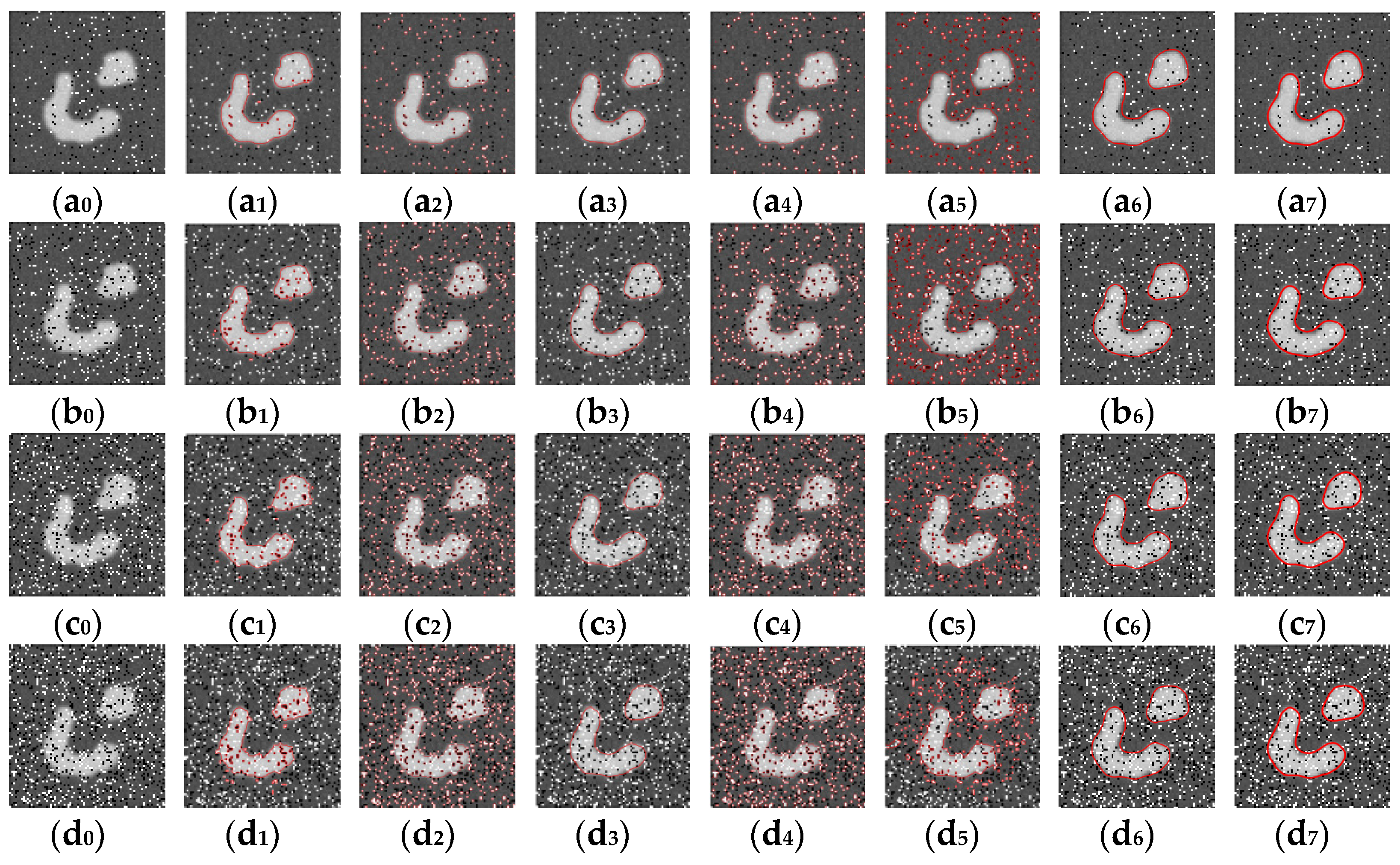
The synthetic images were compared after adding pretzel noise to them. The NFD-LIF model, LBF model, CV model, LSACM model, LIF model, model from [16], and model from [27] were compared for the experiments, and the segmentation results are shown in Figure 8. Column 1 in Figure 8 shows the pretzel noise images with levels of 0.2, 0.4, 0.6, and 0.8. Columns 2 to 7 show the segmentation results of the LBF model, CV model, model from [16], LIF model, LSACM model, and model from [27], respectively, and column 8 shows the segmentation results of the NFD-LIF model.

Figure 8 shows the visual observation of images (a₀,b₀,c₀,d₀), where the foreground of image (a₀), its size, and its contour shape are very clear. As the noise level increases, the segmentation targets and backgrounds of (b₀), (c₀), and (d₀) are gradually eroded, and their sizes, as well as contour shapes, are gradually blurred. The degree of blurring poses certain difficulties for the segmentation task. The LBF model, CV model, LIF model, and LSACM model were more sensitive to the pretzel noise and did not segment the targets. The main reasons why these models were sensitive to the pretzel noise are as follows: on the one hand, the energy generalization function of these models is inscribed by using L2 parametric or Gaussian fitting functions; on the other hand, the fractional-order filter operator is not considered when constructing these models, although the fractional-order filter operator can extract more texture detail information compared to the integer-order operator. With the increasing noise corruption, the model from [16] extracted the target boundary, but the segmentation was not accurate enough. The model from [27] and the NFD-LIF model extracted the target boundary not only when the foreground and background were clear, but also when the foreground and background were corrupted, and the extracted boundary was smooth. Therefore, both the model from [27] and the NFD-LIF model obtained better segmentation results and were robust to pretzel noise, while the LBF model, CV model, LIF model, LSACM model, and model from [16] were more sensitive to pretzel noise, which led to a decrease in the segmentation accuracy or even an inability to perform complete segmentation. To demonstrate the segmentation performance and efficiency of the various models, the comparison results of their iteration numbers and running times are shown in

Table 3. Comparison of Model Segmentation Running Times and Number of Iterations for Different Pretzel Noise Levels on Structurally Information-Rich Images.

Model	0.05		0.10		0.15		0.20
	Time (s)	Iterations	Time (s)	Iterations	Time (s)	Iterations	Time (s)	Iterations
LBF	34.074	40	41.697	50	59.556	70	60.451	70
CV	2.408	80	2.728	100	3.466	150	5.565	300
Model from [16]	1.018	50	1.199	80	1.433	120	1.129	150
LIF	4.682	600	4.987	700	5.082	700	5.875	800
LSACM	5.438	300	6.808	400	8.728	600	11.139	800
Model from [27]	14.507	290	14.545	300	14.512	300	16.479	350
NFD-LIF	2.748	17	3.183	20	3.260	25	3.272	25

.

The image segmentation task was to compare the segmentation performance and efficiency of the various models provided that the target boundaries could be extracted accurately. As can be seen from Table 3, for different levels of pretzel noise, although the model from [16] and the CV model have a shorter runtime than the NDF-LIF model, the segmentation of both models is not as good as the NDF-LIF model from Figure 7, especially for targets with more complex boundaries, where neither model performs accurate segmentation. For the segmentation results of the model from [27], despite being able to extract the target accurately, its number of iterations far exceeds that of the NFD-LIF model, so the NFD-LIF model outperforms the literature [27] both in the runtime dimension and its iteration count dimension. Additionally, for the other models, the NFD-LIF model outperforms the other models in terms of segmentation, both in Figure 7 and in Table 3.

Pretzel noise was applied to real images, and then the images were compared. The NFD-LIF model, LBF model, LIF model, HLFRA model, GLFIF model, and models from [16,27] were compared for the experiment with pretzel noise images with levels of 0.05 and 0.2, and the segmentation results are shown in Figure 9.

The first row of Figure 9 shows that the model from [27] and the NFD-LIF model extracted the target boundary and that the extracted boundary was smooth. In contrast, the LBF model, LIF model, HLFRA model, GLFIF model, and model from [16] were more sensitive to the pretzel noise, which led to a decrease in the segmentation accuracy and an inability to extract the target boundary. As shown by the second row of Figure 10, with the noise corruption becoming increasingly serious, the NFD-LIF model extracted the target boundary, and the extracted boundary was smooth. In contrast, the LBF model, LIF model, HLFRA model, GLFIF model, and models from [16,27] were more sensitive to the pretzel noise, which led to the degradation of the segmentation accuracy and an inability to achieve the desired segmentation results. As can be seen from Figure 9, the segmentation effect of the model from [27] was not ideal when the pretzel noise intensity was 0.2. In particular, the LBF model, LIF model, and HLFRA model exhibited the worst segmentation effect. In contrast, the NFD-LIF model extracted the target boundary, and the extracted boundary was smooth and had some robustness to the pretzel noise

4.2. Segmentation Results of the Model for Texture Information-Rich Images

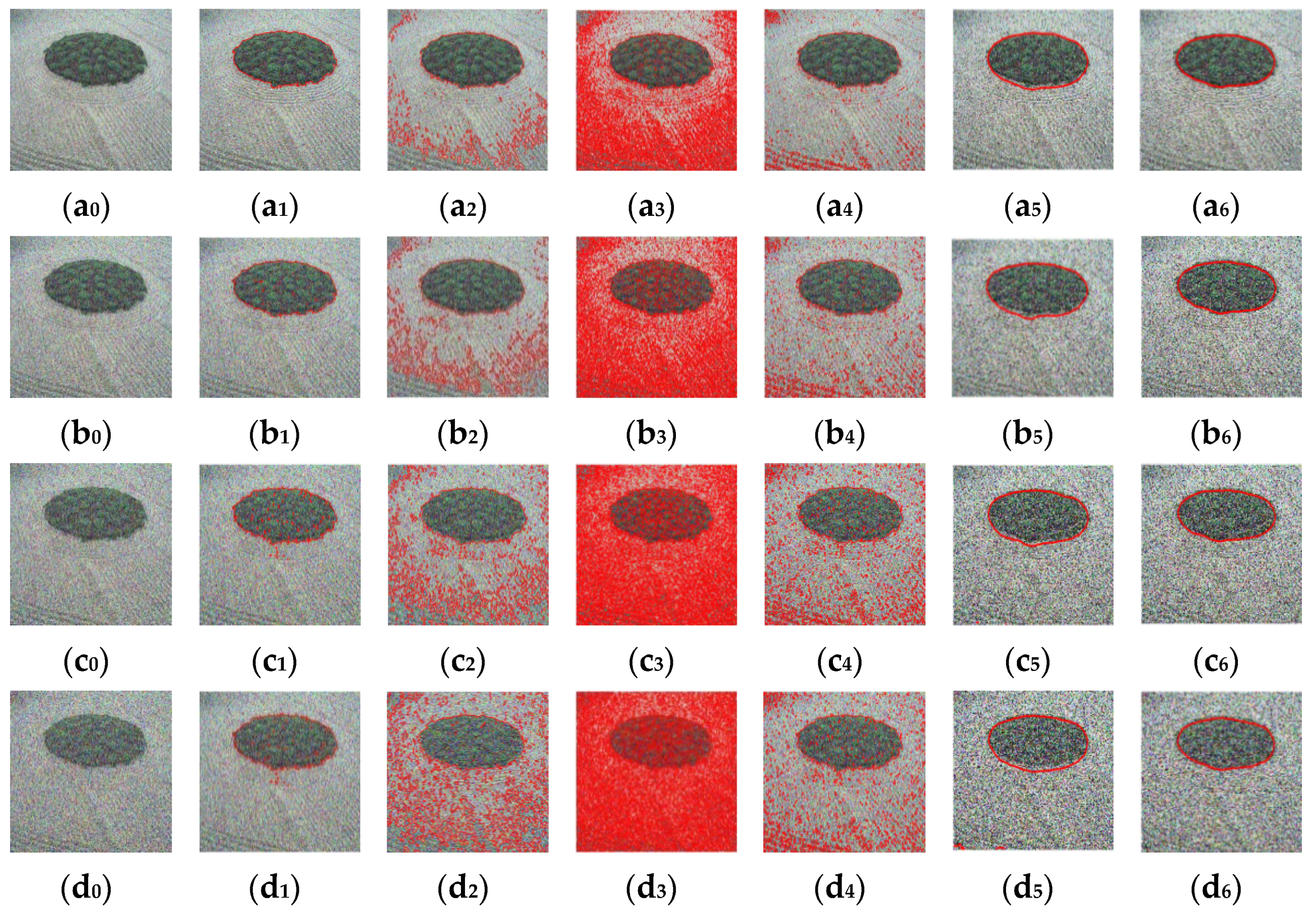
To verify the robustness of the NFD-LIF model against noise, natural images with pretzel noise were compared. The NFD-LIF model, LIC model, LIF model, ACM-LPF model, LSACM model, and model from [27] were compared for the experiments. In Figure 10, column 1 shows the pretzel noise images with levels of 0.1, 0.2, 0.3, and 0.4; columns 2 to 6 are the segmentation results for the LIC model, LIF model, ACM-LPF model, LSACM model, and model from [27]; and column 7 shows the segmentation results of the NFD-LIF model.

Figure 10. Image segmentation results for different pretzel noise levels: (a₀,b₀,c₀,d₀) are images with pretzel noise levels of 0.1, 0.2, 0.3, and 0.4, respectively. (a₁,b₁,c₁,d₁) are the LIC model segmentation results; (a₂,b₂,c₂,d₂) are the LIF model segmentation results. (a₃,b₃,c₃,d₃) are the ACM-LPF model segmentation results. (a₄,b₄,c₄,d₄) are the results of the LSACM model segmentation. (a₅,b₅,c₅,d₅) are the results of the segmentation using the model from [27]. (a₆,b₆,c₆,d₆) are the results of the NFD-LIF model segmentation.

Figure 10. Image segmentation results for different pretzel noise levels: (a₀,b₀,c₀,d₀) are images with pretzel noise levels of 0.1, 0.2, 0.3, and 0.4, respectively. (a₁,b₁,c₁,d₁) are the LIC model segmentation results; (a₂,b₂,c₂,d₂) are the LIF model segmentation results. (a₃,b₃,c₃,d₃) are the ACM-LPF model segmentation results. (a₄,b₄,c₄,d₄) are the results of the LSACM model segmentation. (a₅,b₅,c₅,d₅) are the results of the segmentation using the model from [27]. (a₆,b₆,c₆,d₆) are the results of the NFD-LIF model segmentation.

Figure 10 shows that the LIC model, LIF model, ACM-LPF model, and LSACM model were more sensitive to the pretzel noise, which led to a decrease in the segmentation accuracy and an inability to achieve the desired segmentation results or even complete segmentation. Although the model from [27] extracted the target boundary, under-segmentation occurred, which eventually led to segmentation failure. In contrast, the NFD-LIF model could extract the target boundary, and it could extract the boundary smoothly. Therefore, the NFD-LIF model had some robustness to the pretzel noise. To demonstrate the performance and efficiency, the comparison results of the number of iterations and running time are shown in

Table 4. Comparison of Model Segmentation Running Times and Number of Iterations for Different Pretzel Noise Levels on Texture Information-Rich Images.

Model	0.1		0.2		0.3		0.4
	Time (s)	Iterations	Time (s)	Iterations	Time (s)	Iterations	Time (s)	Iterations
LIC	84.187	200	93.161	220	109.747	260	168.315	400
LIF	269.597	300	371.972	400	469.276	500	683.124	700
ACM-LPF	247.853	200	251.804	200	261.478	300	273.04	400
LSACM	405.048	300	526.808	400	787.107	600	1057.725	800
Model from [27]	11.450	70	11.938	70	12.561	70	21.579	150
NFD-LIF	5.89	30	6.628	30	7.601	30	9.780	60

.

According to Table 4, the ACM-LPF model segmented the natural images with pretzel noise with the highest processing time, but the segmentation outcomes were also the worst. In contrast, the LIC model, LIF model, and LSACM model segmented the natural images with pretzel noise with fewer iterations, but the segmentation outcomes were not satisfactory. On the other hand, the NFD-LIF model segmented images with various levels of pretzel noise the best and required the fewest iterations and shortest running time.

For comparison trials, Gaussian noise was applied to the images in order to further demonstrate the NFD-LIF model’s robustness against noise. Figure 11 displays the segmentation outcomes. The models used in the trials included the NFD-LIF model, LIC model, LIF model, HLFRA model, GLFIF model, model from [16], and model from [27].

The top row of Figure 11 demonstrates that the recovered boundary from the NFD-LIF model and the model from [27] was smooth and that these models were able to extract the target boundary. The target boundary could not be extracted using the LIC model, LIF model, HLFRA model, GLFIF model, or model from [16], which were more susceptible to the Gaussian noise. The NFD-LIF model extracted the target boundary with increasing noise corruption, as seen in the second row of Figure 10, and the extracted boundary was similarly smooth. Additionally, the models from [16,27] were able to extract the desired border; however, over-segmentation occurred with the model from [16], while under-segmentation occurred with the model from [27], which ultimately resulted in the segmentation task failing. The target boundary could not be extracted by the LIC model, LIF model, HLFRA model, or GLFIF model since they were more sensitive to the Gaussian noise. Figure 11 illustrates how progressively susceptible to the Gaussian noise the LIC model, LIF model, HLFRA model, GLFIF model, and models from [16,27] were, and how they were even unable to execute a full segmentation. The NFD-LIF model, on the other hand, was somewhat resistant to the Gaussian noise.

5. Conclusions

In this paper, we proposed an NFD-LIF segmentation model based on the coupling of the local spectral histogram and fractional-order gradient information. The model primarily uses factorization theory to solve the weight function while simultaneously building the fitting image of the energy generalization using fractional-order differentiation and constraining the level set function by the regular parameter to improve the segmentation accuracy of high-noise images. The experimental results demonstrate that the NFD-LIF model could accurately segment images with various levels of noise and that the segmentation outcomes were unaffected by the initial contour position, size, and shape. In addition, on the premise that the object boundary can be accurately extracted, the NFD-LIF model ran faster and required fewer iterations than the classical model. The disadvantage of the proposed model is that there is no adaptive selection of parameters in the process of building the model.

References

1. Dai, J.; He, K.; Sun, J. Instance-aware semantic segmentation via multi-task network cascades. In Proceedings of the IEEE Conference on Computer Vision and Pattern Recognition (CVPR), Las Vegas, NV, USA, 27–30 June 2016; pp. 3150–3158. [Google Scholar]
2. Chen, L.C.; Papandreou, G.; Kokkinos, I.; Murphy, K.; Yuille, A.L. Semantic image segmentation with deep convolutional nets and fully connected CRFs. Comput. Sci. 2014, 4, 357–361. [Google Scholar]
3. Chen, L.C.; Papandreou, G.; Kokkinos, I.; Murphy, K.; Yuille, A.L. DeepLab: Semantic image segmentation with deep convolutional nets, atrous convolution, and fully connected CRFs. IEEE Trans. Pattern Anal. Mach. Intell. 2018, 40, 834–848. [Google Scholar] [CrossRef] [PubMed]
4. Chen, L.C.; Papandreou, G.; Schroff, F. Rethinking atrous convolution for semantic image segmentation. In Proceedings of the IEEE Conference on Computer Vision and Pattern Recognition (CVPR), Honolulu, HI, USA, 21–26 July 2017; pp. 851–859. [Google Scholar]
5. Chen, L.; Zhu, Y.; Papandreou, G.; Schroff, F.; Adam, H. Encoder-decoder with atrous separable convolution for semantic image segmentation. In Proceedings of the European Conference on Computer Vision (ECCV), Munich, Germany, 8–14 September 2018; pp. 801–818. [Google Scholar]
6. Chen, X.; Williams, B.M.; Vallabhaneni, S.R.; Czanner, G.; Zheng, Y. Learning active contour models for medical image segmentation. In Proceedings of the IEEE/CVF Conference on Computer Vision and Pattern Recognition (CVPR), Long Beach, CA, USA, 1–20 June 2019. [Google Scholar]
7. Jie, D.; Ying, Z.; Amjad, A.; Jiao, F.X.; Thill, D.M.S.; Li, X.A. Automatic contour refinement for deep learning auto-segmentation of complex organs in MRI-guided adaptive radiotherapy. Adv. Radiat. Oncol. 2022, 7, 100968. [Google Scholar]
8. Jiang, Y.; Yeh, W.C.; Hao, Z.; Yang, Z. A cooperative honey bee mating algorithm and its application in multi-threshold image segmentation. Inf. Sci. 2016, 369, 171–183. [Google Scholar] [CrossRef]
9. Liu, C.; Zhao, R.; Pang, M. Lung segmentation based on random forest and multi-scale edge detection. IET Image Processing 2019, 13, 1745–1754. [Google Scholar] [CrossRef]
10. Raj, S.M.A.; Jose, C.; Supriya, M.H. Hardware realization of canny edge detection algorithm for underwater image segmentation using field programmable gate arrays. J. Eng. Sci. Technol. 2017, 12, 2536–2550. [Google Scholar]
11. Liu, C.; Liu, W.; Xing, W. A weighted edge-based level set method based on multi-local statistical information for noisy image segmentation. J. Vis. Commun. Image Represent 2019, 59, 89–107. [Google Scholar] [CrossRef]
12. Zhi, X.H.; Shen, H.B. Saliency driven region-edge-based top down level set evolution reveals the asynchronous focus in image segmentation. Pattern Recognit. 2018, 80, 241–255. [Google Scholar] [CrossRef]
13. Ibrahim, R.W.; Hasan, A.M.; Jalab, H.A. A new deformable model based on fractional wright energy function for tumor segmentation of volumetric brain MRI scans. Comput. Methods Programs Biomed. 2018, 163, 21–28. [Google Scholar] [CrossRef]
14. Liu, H.; Tang, P.; Guo, D.; Liu, H.; Zheng, Y.; Dan, G. Liver MRI segmentation with edge preserved intensity inhomogeneity correction. Signal Image Video Process 2018, 12, 791–798. [Google Scholar] [CrossRef]
15. Panigrahi, L.; Verma, K.; Singh, B.K. Hybrid segmentation method based on multi-scale Gaussian kernel fuzzy clustering with spatial bias correction and region-scalable fitting for breast US images. IET Comput. Vis 2018, 12, 1067–1077. [Google Scholar] [CrossRef]
16. Weng, G.; Dong, B.; Lei, Y. A level set method based on additive bias correction for image segmentation. Expert Syst. Appl. 2021, 185, 115633. [Google Scholar] [CrossRef]
17. Kass, M.; Witkin, A.; Terzopoulos, D. Snakes: Active contour models. Int. J. Comput. Vis. 1988, 1, 321–331. [Google Scholar] [CrossRef]
18. Cselles, V.; Kimmel, R.; Sapiro, G. Geodesic active contours. Int. J. Comput. Vis. 1997, 22, 61–79. [Google Scholar] [CrossRef]
19. Chan, T.F.; Vese, L.A. Active contours without edges. IEEE Trans. Image Processing 2001, 10, 266–277. [Google Scholar] [CrossRef]
20. Li, C.M.; Kao, C.Y.; Gore, J.C.; Ding, Z.H. Minimization of region-scalable fitting energy for image segmentation. IEEE Trans. Image Processing 2008, 17, 1940–1949. [Google Scholar]
21. Zhang, K.; Song, H.; Zhang, L. Active contours driven by local image fitting energy. Pattern Recognit. 2010, 43, 1199–1206. [Google Scholar] [CrossRef]
22. Lee, H.S.; In Cho, S. Spatial color histogram-based image segmentation using texture-aware region merging. Multimed. Tools Appl. 2022, 81, 24573–24600. [Google Scholar] [CrossRef]
23. Min, H.; Jia, W.; Wang, X.F.; Zhao, Y.; Hu, R.X.; Luo, Y.T.; Xue, F.; Lu, J.T. An intensity-texture model based level set method for image segmentation. Pattern Recognit. 2015, 48, 1547–1562. [Google Scholar] [CrossRef]
24. Liu, L.; Fan, S.; Ning, X.; Liao, L. An efficient level set model with self-similarity for texture segmentation. Neurocomputing 2017, 266, 150–164. [Google Scholar] [CrossRef]
25. Subudhi, P.; Mukhopadhyay, S. A novel texture segmentation method based on co-occurrence energy-driven parametric active contour model. Signal Image Video Process 2018, 12, 669–676. [Google Scholar] [CrossRef]
26. Yuan, J.; Wang, D.; Cheriyadat, A.M. Factorization-based texture segmentation. Image Processing IEEE Trans. 2015, 24, 3488–3497. [Google Scholar] [CrossRef] [PubMed]
27. Gao, M.; Chen, H.; Zheng, S.; Fang, B. A factorization based active contour model for texture segmentation. In Proceedings of the IEEE International Conference on Image Processing (ICIP), Phoenix, AZ, USA, 25–28 September 2016; pp. 4309–4313. [Google Scholar]
28. Gao, G.; Wang, H.; Wen, C.; Xu, L. Texture image segmentation using statistical active contours. J. Electron. Imaging 2018, 27, 051211. [Google Scholar] [CrossRef]
29. Shamsi, Z.H.; Kim, D.G.; Hussain, M.; Sajawal, R.M.B.K. Low-rank estimation for image denoising using fractional-order gradient-based similarity measure. Circuits Syst. Signal Processing 2021, 40, 4946–4968. [Google Scholar] [CrossRef]
30. Golbaghi, F.K.; Rezghi, M.; Eslahchi, M.R. A hybrid image denoising method based on integer and fractional-order total variation. Iran. J. Sci. Technology. Trans. A Sci. 2020, 44, 1803–1814. [Google Scholar] [CrossRef]
31. Zhang, Y.S.; Zhang, F.; Li, B.Z.; Tao, R. Fractional domain varying-order differential denoising method. Opt. Eng. 2014, 53, 102102. [Google Scholar] [CrossRef]
32. Khan, M.A.; Ullah, A.; Khan, S.; Ali, M.; Ali, J. A novel fractional-order variational approach for image restoration based on fuzzy membership degrees. IEEE Access 2021, 9, 43574–43600. [Google Scholar] [CrossRef]
33. Gao, X.; Yu, J.; Yan, H.; Mou, J. A new image encryption scheme based on fractional-order hyperchaotic system and multiple image fusion. Sci. Rep. 2021, 11, 15737. [Google Scholar] [CrossRef]
34. Zhang, X.F.; Yan, H.; He, H. Multi-focus image fusion based on fractional-order derivative and intuitionistic fuzzy sets. Front. Inf. Technol. Electron. Eng. 2020, 21, 834–843. [Google Scholar] [CrossRef]
35. Chen, B.; Zou, Q.H.; Chen, W.S.; Li, Y. A fast region-based segmentation model with Gaussian kernel of fractional order. Adv. Math. Phys. 2013, 2013, 501628. [Google Scholar] [CrossRef]
36. Zhang, Y.; Tian, Y. A new active contour medical image segmentation method based on fractional varying-order differential. Mathematics 2022, 10, 206. [Google Scholar] [CrossRef]
37. Li, M.M.; Li, B.Z. A novel active contour model for noisy image segmentation based on adaptive fractional order differentiation. IEEE Trans. Image Processing 2020, 29, 9520–9531. [Google Scholar] [CrossRef] [PubMed]
38. Gu, M.; Wang, R. Fractional differentiation-based active contour model driven by local intensity fitting energy. Math. Probl. Eng. 2016, 2016, 6098021. [Google Scholar] [CrossRef]
39. Arbelaez, P.; Maire, M.; Fowlkes, C.; Malik, J. Contour detection and hierarchical image segmentation. IEEE Trans. Pattern Anal. Mach. Intell. 2011, 33, 898–916. [Google Scholar] [CrossRef] [PubMed]
40. Chen, M.P.; Srivastava, H.M. Fractional calculus operators and their applications involving power functions and summation of series. Appl. Math. Comput. 1997, 81, 287–304. [Google Scholar] [CrossRef]
41. Pu, Y.F.; Zhou, J.L. A novel approach for multi-scale texture segmentation based on fractional differential. Int. J. Comput. Math. 2011, 88, 58–78. [Google Scholar] [CrossRef]
42. Pritpal, S.; Surya, S.B. A quantum-clustering optimization method for COVID-19 CT scan image segmentation. Expert Syst. Appl. 2021, 185, 1–21. [Google Scholar]
43. Shu, X.; Yang, Y.; Wu, B. Adaptive segmentation model for liver CT images based on neural network and level set method. Neurocomputing 2021, 453, 438–452. [Google Scholar] [CrossRef]
44. Saman, S.; Narayanan, S.J. Active contour model driven by optimized energy functionals for MR brain tumor segmentation with intensity inhomogeneity correction. Multimed. Tools Appl. 2021, 80, 21925–21954. [Google Scholar] [CrossRef]
Figure 1. Fractional-order mask operator: (a1,a2) are the positive and negative x-axis directions respectively; (a3,a4) are the positive and negative y-axis directions respectively; (a5,a6) are the lower left and upper right diagonals respectively, (a7,a8) are the upper left and lower right diagonals respectively.
Fractalfract 06 00462 g001
Figure 2. Results of gradient comparison of different images: (a1,b1,c1,d1) are the original images selected for the experiment; (a2,b2,c2,d2) are the integer-order gradient maps corresponding to the original images; (a3,b3,c3,d3) are the fractional-order gradient maps corresponding to the original images.
Fractalfract 06 00462 g002
Figure 3. Segmentation results of the initial rectangular profile: (a0a2) are the original images with different initial contours. (b0b2) is the segmentation result of NFD-LIF model.
Fractalfract 06 00462 g003
Figure 4. Segmentation results of different initial contours: (a0,b0,c0) denote the results of the segmentation of different rectangular initial contours; (a1,b1,c1) denote the results of the segmentation of different circular initial contours; (a2,b2,c2) denote the results of the segmentation of different triangular initial contours; (a3,b3,c3) denote the results of the segmentation of different trapezoidal initial contours results.
Fractalfract 06 00462 g004
Figure 5. Image segmentation results with different noise levels: (a0,b0) are images with Gaussian noise with a mean of 0 and variances of 0.05 and 0.2, respectively. (c0,d0) are images with pretzel noise with levels of 0.2 and 0.8, respectively. (a1d1) are the segmentation results corresponding to (a0d0), respectively.
Fractalfract 06 00462 g005
Figure 6. Segmentation results of natural images: (a0a5) are six different scene segmentation maps without adding noise; (b0b5) are six different scene segmentation maps with different noise levels.
Fractalfract 06 00462 g006
Figure 7. Image segmentation results for different Gaussian noise levels: (a0,b0,c0,d0) are Gaussian noise images with a mean of 0 and variances of 0.01, 0.05, 0.09, and 0.13, respectively. (a1,b1,c1,d1) are the segmentation results of the LIC model. (a2,b2,c2,d2) are the segmentation results of the LBF model. (a3,b3,c3,d3) are the segmentation results of the model from [16]. (a4,b4,c4,d4) are results of the model from [27]. (a5,b5,c5,d5) are results of the NFD-LIF model.
Fractalfract 06 00462 g007
Figure 8. Image segmentation results for different levels of pretzel noise: (a0,b0,c0,d0) are pretzel noise images with levels of 0.2, 0.4, 0.6, and 0.8, respectively. (a1,b1,c1,d1) are the results of the LBF model segmentation. (a2,b2,c2,d2) are the results of the CV model segmentation. (a3,b3,c3,d3) are the results of the segmentation using the model from [16]. (a4,b4,c4,d4) are the results of the LIF model segmentation. (a5,b5,c5,d5) are the results of the LSACM model segmentation. (a6,b6,c6,d6) are the results of the segmentation using the model from [27]. (a7,b7,c7,d7) are the results of the NFD-LIF model segmentation.
Fractalfract 06 00462 g008
Figure 9. Image segmentation results for different pretzel noise levels: (a0,b0) are pretzel noise images with levels of 0.05 and 0.2, respectively. (a1,b1) are the results of the segmentation using the model from [16]. (a2,b2) are the results of the HLFRA model segmentation. (a3,b3) are the results of the GLFIF model segmentation. (a4,b4) are the results of the LBF model segmentation. (a5,b5) are the results of the LIF model segmentation; (a6,b6) are the results of the segmentation using the model from [27]. (a7,b7) are the results of the NFD-LIF model segmentation.
Fractalfract 06 00462 g009
Figure 11. Segmentation results of Gaussian noise images with different levels: (a0,b0) are the Gaussian noise images with a mean of 0 and variances of 0.08 and 0.1, respectively. (a1,b1) are the results of the segmentation using the model from [16]. (a2,b2) are the results of the HLFRA model segmentation; (a3,b3) are the results of the GLFIF model segmentation. (a4,b4) are the results of the LIC model segmentation. (a5,b5) are the results of the LIF model segmentation. (a6,b6) are the results of the segmentation using the model from [27]. (a7,b7) are the results of the NFD-LIF model segmentation.
Fractalfract 06 00462 g011