
A Numerical Strategy for the Approximate Solution of the Nonlinear Time-Fractional Foam Drainage Equation


Abstract
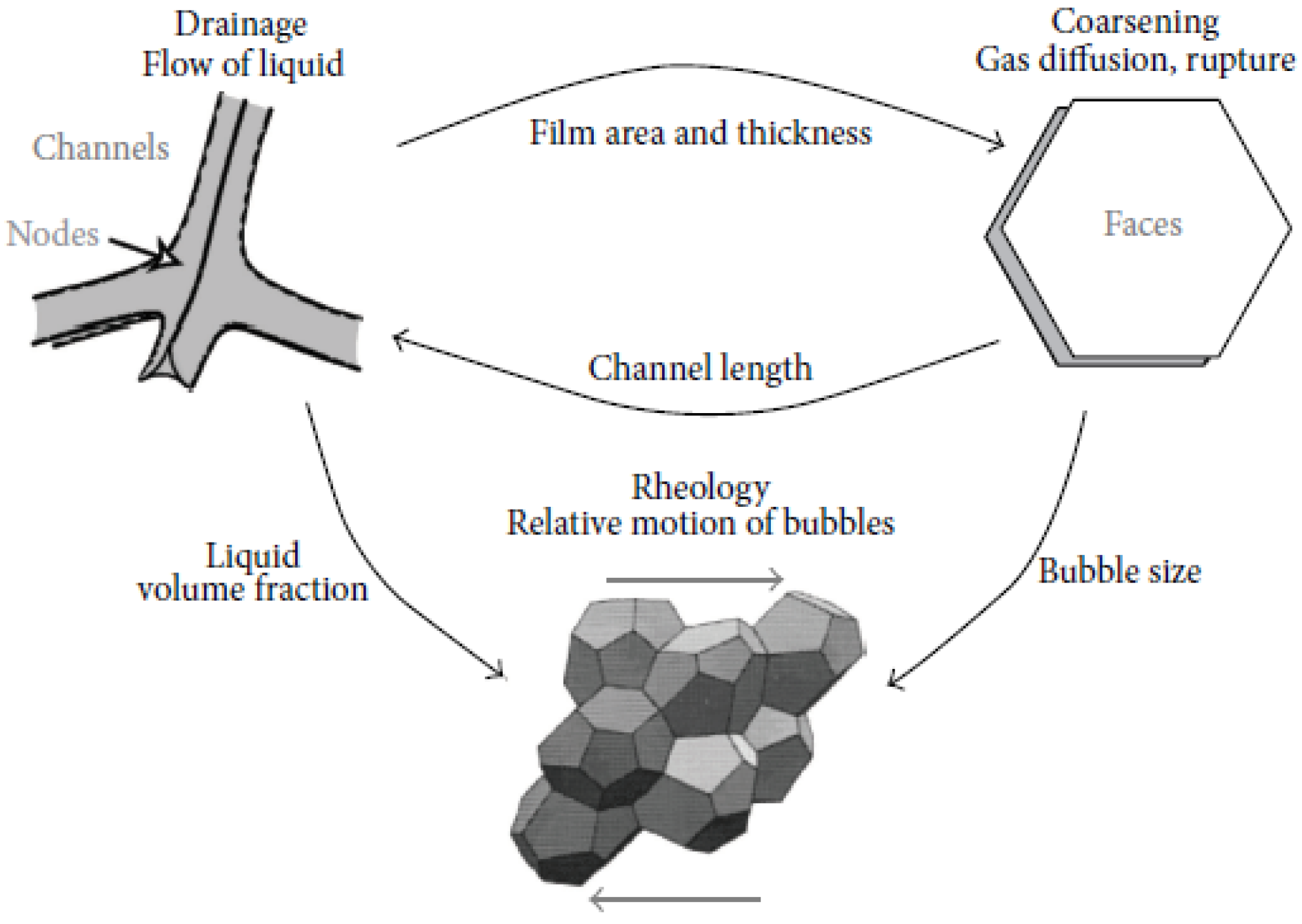
1. Introduction
2. Preliminaries
3. Basic Idea of LHPTM
- (i)
- The second order derivative of according to should be smaller as the parameter p becomes larger, i.e.,
- (ii)
- , so that the series converges, whereas represents the inverse of the linear operator .
4. Convergence Analysis
- (1)
- ;
- (2)
- is forever in the neighborhood of meaning
- (3)
- .
- ;
- whatever may be , there exists a constant such that for with , we have for every .
5. Numerical Applications
5.1. Example 1
5.2. Example 2
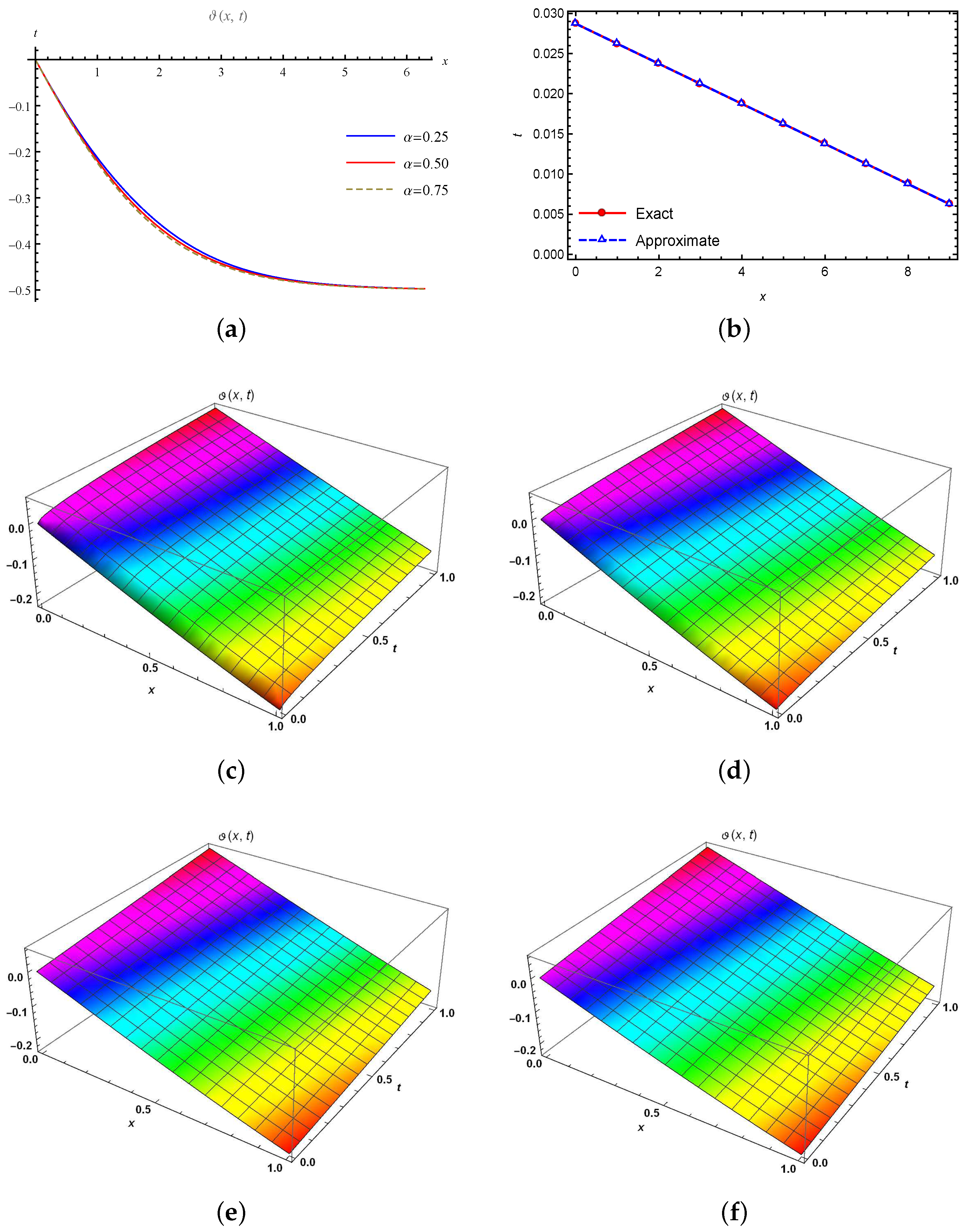
6. Results and Discussion
7. Conclusions
Author Contributions
Funding
Institutional Review Board Statement
Informed Consent Statement
Data Availability Statement
Conflicts of Interest
References
- Kilbas, A.A.; Srivastava, H.M.; Trujillo, J.J. Theory and Applications of Fractional Differential Equations; Elsevier: New York, NY, USA, 2006; Volume 204. [Google Scholar]
- Wazwaz, A.M. New integrable (2+1)-and (3+1)-dimensional shallow water wave equations: Multiple soliton solutions and lump solutions. Int. J. Numer. Methods Heat Fluid Flow 2021, 32, 138–149. [Google Scholar] [CrossRef]
- Nadeem, M.; He, J.H. He–Laplace variational iteration method for solving the nonlinear equations arising in chemical kinetics and population dynamics. J. Math. Chem. 2021, 59, 1234–1245. [Google Scholar] [CrossRef]
- Habib, S.; Islam, A.; Batool, A.; Sohail, M.U.; Nadeem, M. Numerical solutions of the fractal foam drainage equation. GEM Int. J. Geomath. 2021, 12, 1–10. [Google Scholar] [CrossRef]
- Islam, S.; Alam, M.N.; Al-Asad, M.F.; Tunç, C. An analytical technique for solving new comoutational solutions of the Modified Zakharov-Kuznetsov equation arising in electrical enfineering. J. Appl. Comput. Mech. 2021, 7, 715–726. [Google Scholar]
- Alam, M.N. Exact solutions to the foam drainage equation by using the new generalized (G′/G)-expansion method. Results Phys. 2015, 5, 168–177. [Google Scholar] [CrossRef]
- Dahmani, Z.; Anber, A. The variational iteration method for solving the fractional foam drainage equation. Int. J. Nonlinear Sci. 2010, 10, 39–45. [Google Scholar]
- Khani, F.; Hamedi-Nezhad, S.; Darvishi, M.; Ryu, S.W. New solitary wave and periodic solutions of the foam drainage equation using the Exp-function method. Nonlinear Anal. Real World Appl. 2009, 10, 1904–1911. [Google Scholar] [CrossRef]
- Alquran, M. Analytical solutions of fractional foam drainage equation by residual power series method. Math. Sci. 2014, 8, 153–160. [Google Scholar] [CrossRef]
- Jena, R.M.; Chakraverty, S.; Jena, S.K.; Sedighi, H.M. Analysis of time-fractional fuzzy vibration equation of large membranes using double parametric based Residual power series method. ZAMM J. Appl. Math. Mech. Angew. Math. Mech. 2021, 101, e202000165. [Google Scholar] [CrossRef]
- Fereidoon, A.; Yaghoobi, H.; Davoudabadi, M. Application of the homotopy perturbation method for solving the foam drainage equation. Int. J. Differ. Equ. 2011, 2011, 864023. [Google Scholar] [CrossRef]
- Darvishi, M.; Khani, F. A series solution of the foam drainage equation. Comput. Math. Appl. 2009, 58, 360–368. [Google Scholar] [CrossRef][Green Version]
- Arbabi, S.; Nazari, A.; Darvishi, M.T. A semi-analytical solution of foam drainage equation by Haar wavelets method. Optik 2016, 127, 5443–5447. [Google Scholar] [CrossRef]
- Nadeem, M.; Yao, S.W. Solving the fractional heat-like and wave-like equations with variable coefficients utilizing the Laplace homotopy method. Int. J. Numer. Methods Heat Fluid Flow 2020, 31, 273–292. [Google Scholar] [CrossRef]
- Gupta, S.; Kumar, D.; Singh, J. Analytical solutions of convection–diffusion problems by combining Laplace transform method and homotopy perturbation method. Alex. Eng. J. 2015, 54, 645–651. [Google Scholar] [CrossRef]
- Johnston, S.; Jafari, H.; Moshokoa, S.; Ariyan, V.; Baleanu, D. Laplace homotopy perturbation method for Burgers equation with space-and time-fractional order. Open Phys. 2016, 14, 247–252. [Google Scholar] [CrossRef]
- Madani, M.; Fathizadeh, M.; Khan, Y.; Yildirim, A. On the coupling of the homotopy perturbation method and Laplace transformation. Math. Comput. Model. 2011, 53, 1937–1945. [Google Scholar] [CrossRef]
- Caponetto, R. Fractional Order Systems: Modeling and Control Applications; World Scientific: Singapore, 2010; Volume 72. [Google Scholar]
- Milici, C.; Drăgănescu, G.; Machado, J.T. Introduction to Fractional Differential Equations; Springer: Berlin/Heidelberg, Germany, 2018; Volume 25. [Google Scholar]
- Zhou, Y.; Wang, J.; Zhang, L. Basic Theory of Fractional Differential Equations; World Scientific: Singapore, 2016. [Google Scholar] [CrossRef]
- Eslami, M.; Mirzazadeh, M. Study of convergence of Homotopy perturbation method for two-dimensional linear Volterra integral equations of the first kind. Int. J. Comput. Sci. Math. 2014, 5, 72–80. [Google Scholar] [CrossRef]
- He, J.H. Homotopy perturbation technique. Comput. Methods Appl. Mech. Eng. 1999, 178, 257–262. [Google Scholar] [CrossRef]
- Nadeem, M.; Li, F.; Ahmad, H. Modified Laplace variational iteration method for solving fourth-order parabolic partial differential equation with variable coefficients. Comput. Math. Appl. 2019, 78, 2052–2062. [Google Scholar] [CrossRef]


| x | Exact | |||
|---|---|---|---|---|
| 0.01 | 0.315188 | 0.291273 | 0.187715 | 0.187746 |
| 0.02 | 0.309270 | 0.282554 | 0.178066 | 0.178081 |
| 0.03 | 0.303405 | 0.273793 | 0.168371 | 0.168381 |
| 0.04 | 0.297590 | 0.264991 | 0.158649 | 0.158649 |
| 0.05 | 0.294341 | 0.256149 | 0.148896 | 0.148885 |
Publisher’s Note: MDPI stays neutral with regard to jurisdictional claims in published maps and institutional affiliations. |
© 2022 by the authors. Licensee MDPI, Basel, Switzerland. This article is an open access article distributed under the terms and conditions of the Creative Commons Attribution (CC BY) license (https://creativecommons.org/licenses/by/4.0/).
Share and Cite
Liu, F.; Liu, J.; Nadeem, M. A Numerical Strategy for the Approximate Solution of the Nonlinear Time-Fractional Foam Drainage Equation. Fractal Fract. 2022, 6, 452. https://doi.org/10.3390/fractalfract6080452
Liu F, Liu J, Nadeem M. A Numerical Strategy for the Approximate Solution of the Nonlinear Time-Fractional Foam Drainage Equation. Fractal and Fractional. 2022; 6(8):452. https://doi.org/10.3390/fractalfract6080452
Chicago/Turabian StyleLiu, Fenglian, Jinxing Liu, and Muhammad Nadeem. 2022. "A Numerical Strategy for the Approximate Solution of the Nonlinear Time-Fractional Foam Drainage Equation" Fractal and Fractional 6, no. 8: 452. https://doi.org/10.3390/fractalfract6080452
APA StyleLiu, F., Liu, J., & Nadeem, M. (2022). A Numerical Strategy for the Approximate Solution of the Nonlinear Time-Fractional Foam Drainage Equation. Fractal and Fractional, 6(8), 452. https://doi.org/10.3390/fractalfract6080452