Error Bounds of a Finite Difference/Spectral Method for the Generalized Time Fractional Cable Equation

Abstract

We present a finite difference/spectral method for the two-dimensional generalized time fractional cable equation by combining the second-order backward difference method in time and the Galerkin spectral method in space with Legendre polynomials. Through a detailed analysis, we demonstrate that the scheme is unconditionally stable. The scheme is proved to have $\min \{2-\alpha ,2-\beta \}$-order convergence in time and spectral accuracy in space for smooth solutions, where $\alpha ,\beta$ are two exponents of fractional derivatives. We report numerical results to confirm our error bounds and demonstrate the effectiveness of the proposed method. This method can be applied to model diffusion and viscoelastic non-Newtonian fluid flow.

1. Introduction

In recent years, with the fractional differential equations (FDEs) being widely applied in various fields of science and engineering [1], fractional calculus has attracted extensive attention. Furthermore, due to the inherent non-local properties of fractional integrals and derivatives, FDEs have been proven to be more appropriate than integer-order differential equations in describing the memory and hereditary properties of some phenomena and processes in many fields [2], such as physics, chemistry, biology, materials, economics, mechanical engineering, signal processing, systems identification, control theory, and so on [3,4].

Nowadays, fractional calculus has been extensively applied in the modeling of the phenomena of anomalous diffusion in a specific type of porous medium [5] and viscoelastic fluid flow. Consequently, the study of analytical and numerical solutions of FDEs has attracted increasing attention. The fractional cable equation was derived from the Nernst–Planck equation, which modeled electronic properties in spiny neuronal dendrites [6]. Due to its significant deviation from the dynamics of Brownian motion, the anomalous diffusion in biological systems cannot be adequately described by the traditional Nernst–Planck equation or its simplification, the traditional cable equation [6,7]. Subsequently, the time/space fractional cable equation was derived for modeling the electro-diffusion of ions in nerve cells, when the molecular diffusion process is one of anomalous subdiffusion due to binding, crowding, or trapping [8]. The Rayleigh–Stokes/Stokes’ first problem for a generalized second-grade fluid plays an important role in the description of the behavior of some non-Newtonian fluids [9,10,11]. Because of the practical importance of Stokes’ first problem for a heated flat plate, as well as that of the Rayleigh–Stokes problem for a heated edge [12], they have been widely used to investigate different problems, for example, in describing the flow of an Oldroyd-B fluid over a suddenly moved flat plate [13], studying the Oldroyd-B fluid in a heated boundary second-grade fluid in a porous half-space [14], in the case of a Newtonian fluid in a non-Darcian porous half-space [15], etc.

In this paper, we consider the following two-dimensional (2D) generalized time fractional cable equation, which can be simplified as the fractional cable equation and a heated generalized second-grade fluid model in the special case

$${\partial }_{t}u=-a_0\left({}_0{D}_t^{1-{\gamma }_1}u\right)+\left({}_0{D}_t^{1-{\gamma }_2}{a}_1\mathsf{\Delta }u\right)+a_2\mathsf{\Delta }u+f(\mathbf{x},t),\mathbf{x}\in \mathsf{\Omega },t\in I,$$

(1)

with the initial condition

$$u(\mathbf{x},0)=u^0\left(\mathbf{x}\right),\mathbf{x}\in \overline{\mathsf{\Omega }}=\mathsf{\Omega }\cup \partial \mathsf{\Omega },$$

(2)

and the boundary condition

$$u(\mathbf{x},t)=0,(\mathbf{x},t)\in \partial \mathsf{\Omega }\times I,$$

(3)

where $u=u(\mathbf{x},t)$ denotes the 2D velocity, $\mathbf{x}=(x,y),$ $\mathsf{\Omega }=(-L,L)\times (-L,L),$ $I=(0,T];\mathsf{\Delta }u={\partial }_{xx}u+{\partial }_{yy}u,a_0,a_1,a_2$ are positive constants; and $u^0\left(\mathbf{x}\right)$ and $f(\mathbf{x},t)$ are sufficiently smooth functions. When $a_2=0$, this model can be reduced to the 2D fractional cable equation [16,17,18,19,20]. If $a_0=0$, it can be simplified as the 2D Rayleigh–Stokes problem for a heated generalized second-grade fluid model [9,12,21,22,23,24,25]. When $\mathbf{x}=(x,0)$, the 2D generalized fractional cable equation can be reduced to the 1D model; then it can be simplified to the 1D fractional cable equation [26,27,28,29,30,31] for $a_2=0$ and the 1D Stokes’ first problem for heated generalized second-grade fluid model [10,14,32,33] for $a_0=0$. Here the derivative ${}_0{D}_t^{1-\gamma }(0<\gamma <1)$ is the Riemann–Liouville fractional derivative defined by Podlubny [34]

$${}_0{D}_t^{1-\gamma }u(\mathbf{x},t)=\frac{1}{\mathsf{\Gamma }\left(\gamma \right)}\frac{\partial }{\partial t}{\int }_0^t\frac{u(\mathbf{x},\eta )}{{(t-\eta )}^{1-\gamma }}d\eta ,$$

in which $\mathsf{\Gamma }(·)$ is the Gamma function.

Some researchers have tried to construct analytical solutions for the above two types of models. For example, Langlands and Henry [8] introduced fractional Nernst–Planck equations, derived fractional cable equations, and obtained solutions in infinite cables and semi-infinite cables. They also presented the fundamental solutions of two fractional cable equations which modeled the subdiffusion in two ways on infinite and semi-infinite domains [26]. Li and Deng [27] derived the analytical solutions via the integral transform method of the time-space fractional cable equation. Shen et al. [12] investigated the Rayleigh–Stokes problem for a heated generalized second-grade fluid model, and they also obtained its exact solution by using the Fourier transform and fractional Laplace transform. Tan and Masuoka [14] applied Fourier sine transforms to obtain the exact solutions of the velocity and temperature fields of Stokes’ first problem for a second-grade fluid in a porous half-space with a heated boundary. Nazar et al. [32] considered the unsteady flow of a generalized second-grade fluid through an infinite straight circular cylinder.

However, because of the complex properties of the exact solution, analytical methods do not work well for most FDEs, so it is worthwhile to develop numerical methods. Several methods have been developed for solving the fractional cable equation and the generalized second-grade fluid model numerically, such as finite difference methods (FDMs), finite element methods (FEMs), spectral methods, and other methods. As for finite difference methods (FDMs), Liu et al. [28] proposed two new implicit numerical methods for the fractional cable equation and investigated their stability and convergence using the energy method. Hu and Zhang [29] developed two implicit compact difference schemes for the fractional cable equation, and discussed the stability and convergence of the first scheme. Chen et al. [30] utilized Fourier analysis to analyze the convergence and stability of a variable-order nonlinear cable equation. Yu and Jiang [16] proposed a fourth-order compact FDM for the two-dimensional fractional cable equation and investigated the inverse problem of the identification for the fractional derivatives. Chen et al. [9,21] proposed a Fourier method and an extrapolation technique to study the 1D Stokes’ first problem for a heated generalized second-grade fluid, and they also used explicit and implicit FDM to analyze the 2D Rayleigh–Stokes problem for a heated generalized second-grade fluid with fractional derivatives. Mohebbi et al. [22] investigated the compact finite difference scheme and radial basis function (RBF) meshless approach for solving the 2D fractional Rayleigh–Stokes equations of a heated generalized second-grade fluid model. Regarding finite element methods (FEMs), Zhuang et al. [31] simulated the fractional cable equation by means of a Galerkin FEM and verified its theoretical analysis. Liu et al. [17] solved a nonlinear fractional cable equation with a two-grid algorithm combined with FEM. Dehghan and Abbaszadeh [23] employed the Galerkin FEM for the 2D Rayleigh–Stokes problem of a heated generalized second-grade fluid. Bazhlekova et al. [9] investigated the Galerkin FEM in a semi-discrete scheme and two types of FDM in full discrete schemes of the homogeneous problem for the Rayleigh–Stokes equation of a generalized second-grade fluid. Furthermore, concerning spectral methods, Zhang et al. [18] used the discrete-time orthogonal spline collocation method for the 2D fractional cable equation. Bhrawy and Zaky [19] proposed the spectral collocation method for solving one- and two-dimensional variable-order fractional nonlinear cable equations based on the shifted Jacobi collocation procedure in conjunction with the shifted Jacobi operational matrix for variable-order fractional derivatives. Abdelkawy and Alqahtani [24] solved the one and two space-dimensional Stokes’ first problems for a heated generalized second-grade fluid using the spectral collocation method. Some other methods have also been employed to solve this problem. For example, Dehghan and Abbaszadeh [20] proposed an error estimate for the extracted numerical scheme using the element-free Galerkin method to solve the fractional cable equation with a Dirichlet boundary condition. Lin and Jiang [33] introduced an algorithm which was based on reproducing kernel theory to obtain the exact solution and numerically solve Stokes’ first problem for a heated generalized second-grade fluid.

Compared to the low-order methods based on the local category, the spectral method [35,36,37,38,39,40] is a high-order method based on the global category, which has exponential rates of convergence and a high level of accuracy. As a result, it is widely applied in the numerical computing of FDEs. Li and Xu [41] proposed Galerkin spectral methods in both temporal and spatial directions for the time fractional diffusion equation. Zeng et al. [42] investigated the 2D Riesz space fractional nonlinear reaction-diffusion equation by developing a new finite difference/spectral method which combined the Crank–Nicolson method in time and an alternating direction-implicit Galerkin–Legendre spectral method in space. Zheng et al. [43] presented a space-time spectral method for the time fractional Fokker–Planck equation and verified its high-order accuracy and efficiency with some numerical results. Lin and Xu [44] proved the stability and convergence of a finite difference/spectral method for the time-fractional diffusion equation. Lin et al. [7] constructed finite difference/Legendre spectral approximations for the fractional cable equation and analyzed their stability and convergence properties. Huang et al. [5] derived a second-order finite difference-spectral method for the space fractional diffusion equations. Similar studies were given elsewhere in the literature [45]. However, few papers have been published on the spectral method, especially for high-dimensional FDEs. This motivated us to generalize the mixed finite difference/spectral method for the 2D generalized time fractional cable equation.

The rest of this paper is arranged as follows. In Section 2, the second-order backward difference method in time and the Galerkin spectral method in space for the generalized time fractional cable Equations (1)–(3) are constructed, then the stability and error bounds of the full-discrete problem are analyzed. In Section 3, the implementation of the spectral method is presented. Some numerical results are provided in Section 4, which support the theoretical analysis and verify the effectiveness of the proposed method. Finally, our conclusions are presented in Section 5.

2. A Full Discretization and Its Error Bounds

In this section, we first construct a full-discrete scheme using the second-order backward difference method in time and the Galerkin spectral method in space, and then we analyze the stability and the error bounds of the fully discretized scheme for the 2D generalized time fractional cable Equations (1)–(3).

To simplify the symbols without losing generality, in the following discussion, we let $1-{\gamma }_1=\alpha ,1-{\gamma }_2=\beta ,u(\mathbf{x},0)=u^0.$ The constant c denotes a generic positive constant independent of any discretization parameters, which is different for different inequalities and equations. Here we consider the case $f\equiv 0$ in the scheme construction and the numerical analysis of the generalized time fractional cable Equations (1)–(3).

According to the relationship between the two definitions provided by Riemann–Liouville and Caputo [34]

$${}_0^{RL}{D}_t^{\alpha }u={}_0^C{D}_t^{\alpha }u+\frac{u^0}{\mathsf{\Gamma }(1-\alpha )t^{\alpha }},0<\alpha <1,$$

(4)

and considering the wide application of the Caputo definition, here we follow the construction idea used in [44] and employ some of the conclusions presented in [7]. Equation (1) can be denoted under the Caputo definition

$${\partial }_{t}u=-a_0\left({}_0^C{D}_t^{\alpha }u\right)-\frac{a_0{u}^0}{\mathsf{\Gamma }(1-\alpha )t^{\alpha }}+a_1\left({}_0^C{D}_t^{\beta }\mathsf{\Delta }u\right)+\frac{a_1}{\mathsf{\Gamma }(1-\beta )t^{\beta }}\mathsf{\Delta }{u}^0+a_2\mathsf{\Delta }u+f.$$

(5)

2.1. A Finite Difference Scheme in Time

Here, we construct a temporal semi-discrete scheme using the finite difference method. Let $t_k=k\tau ,k=0,1,\cdots ,K,$ where $\tau =\frac{T}{K}$ is the time step size, $u(·,·,t_k)=u^k,and{t}_{k+1}=(k+1)\tau .$ Then, for $0\le k\le K-1$, the time fractional derivative term can be approximated by means of the finite difference method

$$\begin{array}{c}{}_0^C{D}_t^{\alpha }u(x,y,t_{k+1})=\frac{1}{\mathsf{\Gamma }(2-\alpha )}{\displaystyle {\displaystyle \sum }_{j=0}^k}{b}_j\frac{u(x,y,t_{k+1-j})-u(x,y,t_{k-j})}{{\tau }^{\alpha }}+r_{\alpha }^{k+1},\hfill \\ {}_0^C{D}_t^{\beta }\mathsf{\Delta }u(x,y,t_{k+1})=\frac{1}{\mathsf{\Gamma }(2-\beta )}{\displaystyle {\displaystyle \sum }_{j=0}^k}{d}_j\frac{\mathsf{\Delta }u(x,y,t_{k+1-j})-\mathsf{\Delta }u(x,y,t_{k-j})}{{\tau }^{\beta }}+r_{\beta }^{k+1},\hfill \end{array}$$

(6)

where $b_j={(j+1)}^{1-\alpha }-j^{1-\alpha },d_j={(j+1)}^{1-\beta }-j^{1-\beta },j=0,1,\cdots ,k,0\le k\le K-1$. The Appendix of [7,46] has proven that $r_{\alpha }^{k+1}\le c{\tau }^{2-\alpha }$ with c depending only on $\underset{(x,y)\in \mathsf{\Omega },\tau \in I}{max}{\partial }_{\tau \tau }u(x,y,\tau )$, a constant measuring ${\partial }_{tt}u$ and $r_{\beta }^{k+1}\le c{\tau }^{2-\beta }$, where c is merely dependent on ${\partial }_{tt}\mathsf{\Delta }u.$

The first-order time derivative term is approximated using the second-order backward difference method. Thus, we obtain

$${\partial }_{t}u(x,y,t_{k+1})=\frac{3u(x,y,t_{k+1})-4u(x,y,t_k)+u(x,y,t_{k-1})}{2\tau }+O\left({\tau }^2\right),k\ge 1,$$

(7)

$${\partial }_{t}u(x,y,t_1)=\frac{u(x,y,t_1)-u(x,y,t_0)}{\tau }+O\left(\tau \right),k=0.$$

(8)

Then we define the difference operator as follows

$$L_t^1{g}^{k+1}=\left\{\begin{array}{c}\frac{g^1-g^0}{\tau },k=0,\hfill \\ \frac{3g^{k+1}-4g^k+g^{k-1}}{2\tau },k\ge 1.\hfill \end{array}\right.$$

(9)

$$L_t^{\alpha }{g}^{k+1}=\frac{1}{\mathsf{\Gamma }(2-\alpha )}\sum _{j=0}^k{b}_j\frac{g^{k+1-j}-g^{k-j}}{{\tau }^{\alpha }},k\ge 0.$$

(10)

$$L_t^{\beta }\mathsf{\Delta }{g}^{k+1}=\frac{1}{\mathsf{\Gamma }(2-\beta )}\sum _{j=0}^k{d}_j\frac{\mathsf{\Delta }{g}^{k+1-j}-\mathsf{\Delta }{g}^{k-j}}{{\tau }^{\beta }},k\ge 0.$$

(11)

According to (5)–(11), we have

$$\begin{array}{c}{L}_t^{1}u(x,y,t_{k+1})\hfill \\ \hfill =& -a_0{L}_t^{\alpha }u(x,y,t_{k+1})+a_1{L}_t^{\beta }\mathsf{\Delta }u(x,y,t_{k+1})\hfill \\ \hfill & +a_2\mathsf{\Delta }u(x,y,t_{k+1})-\frac{a_0}{\mathsf{\Gamma }(1-\alpha ){(k+1)}^{\alpha }{\tau }^{\alpha }}u(x,y,0)\hfill \\ \hfill & +\frac{a_1}{\mathsf{\Gamma }(1-\beta ){(k+1)}^{\beta }{\tau }^{\beta }}\mathsf{\Delta }u(x,y,0)+R^{k+1},k⩾0,\hfill \end{array}$$

(12)

where $R^{k+1}=r_1^{k+1}-a_0{r}_{\alpha }^{k+1}+a_1{r}_{\beta }^{k+1},r_1^{k+1}=O\left(\tau \right)$ for $k=0$, and $r_1^{k+1}=O\left({\tau }^2\right)$ for $k\ge 1$.

Hence, we obtain the finite difference scheme for the time discretization of (5) in $f=0$ as follows.

$$\begin{array}{cc}\hfill L_t^1{u}^{k+1}=& -a_0{L}_t^{\alpha }{u}^{k+1}+a_1{L}_t^{\beta }\mathsf{\Delta }{u}^{k+1}+a_2\mathsf{\Delta }{u}^{k+1}\hfill \\ \hfill & -\frac{a_0}{\mathsf{\Gamma }(1-\alpha ){(k+1)}^{\alpha }{\tau }^{\alpha }}{u}^0+\frac{a_1}{\mathsf{\Gamma }(1-\beta ){(k+1)}^{\beta }{\tau }^{\beta }}\mathsf{\Delta }{u}^0,k⩾0,\hfill \end{array}$$

(13)

where $u^k=u^k(x,y)$ is an approximation of $u(x,y,t_k)$. Then scheme (13) has the truncation error $r_1^{k+1}+r_{\alpha }^{k+1}+r_{\beta }^{k+1}$, and the details are as follows

$$\begin{array}{cc}\hfill \frac{u^1-u^0}{\tau }=-& \frac{a_0}{\mathsf{\Gamma }(2-\alpha ){\tau }^{\alpha }}(u^1-u^0)+\frac{a_1}{\mathsf{\Gamma }(2-\beta ){\tau }^{\beta }}\left(\mathsf{\Delta }{u}^1-\mathsf{\Delta }{u}^0\right)\hfill \\ \hfill +& a_2\mathsf{\Delta }{u}^1-\frac{a_0{u}^0}{\mathsf{\Gamma }(1-\alpha ){\tau }^{\alpha }}+\frac{a_1}{\mathsf{\Gamma }(1-\beta ){\tau }^{\beta }}\mathsf{\Delta }{u}^0,k=0,\hfill \end{array}$$

(14)

$$\begin{array}{cc}\hfill \frac{3u^{k+1}-4u^k+u^{k-1}}{2\tau }=-& \frac{a_0}{\mathsf{\Gamma }(2-\alpha ){\tau }^{\alpha }}\left[u^{k+1}-\sum _{j=0}^{k-1}(b_j-b_{j+1})u^{k-j}-b_k{u}^0\right]\hfill \\ \hfill +& \frac{a_1}{\mathsf{\Gamma }(2-\beta ){\tau }^{\beta }}\left[\mathsf{\Delta }{u}^{k+1}-\sum _{j=0}^{k-1}(d_j-d_{j+1})\mathsf{\Delta }{u}^{k-j}-d_k\mathsf{\Delta }{u}^0\right]\hfill \\ \hfill +& a_2\mathsf{\Delta }{u}^{k+1}-\frac{a_0{u}^0}{\mathsf{\Gamma }(1-\alpha ){(k+1)}^{\alpha }{\tau }^{\alpha }}\hfill \\ \hfill +& \frac{a_1}{\mathsf{\Gamma }(1-\beta ){(k+1)}^{\beta }{\tau }^{\beta }}\mathsf{\Delta }{u}^0,k⩾1.\hfill \end{array}$$

(15)

Thus, from (14) and (15), combining the initial and boundary value conditions, we get

$$\begin{array}{ccc}\hfill u^0(x,y)& =& u^0,(x,y)\in \overline{\mathsf{\Omega }},\hfill \end{array}$$

(16)

$$\begin{array}{ccc}\hfill u^{k+1}(x,y)& =& 0,(x,y,t)\in \partial \mathsf{\Omega }\times I,k\ge 0,\hfill \end{array}$$

(17)

which form the complete semi-discrete problem.

Next we will consider the stability and the error bounds for the full-discrete form of the generalized time fractional cable Equations (1)–(3). We assume that the problem has sufficiently smooth solution.

2.2. Stability and Error Bounds for the Full-Discrete Problem

Here we introduce several definitions of functional spaces endowed with standard norms and inner products that will be used in the following discussion.

$$\begin{array}{c}{H}^1\left(\mathsf{\Omega }\right)=\{v\in L^2\left(\mathsf{\Omega }\right)|{\partial }_{x}v,{\partial }_{y}v\in L^2\left(\mathsf{\Omega }\right)\},\hfill \\ H_0^1\left(\mathsf{\Omega }\right)=\{v\in H^1\left(\mathsf{\Omega }\right)|{\left.v\right|}_{\partial \mathsf{\Omega }}=0\},\hfill \end{array}$$

$$H^m\left(\mathsf{\Omega }\right)=\{v\in L^2\left(\mathsf{\Omega }\right)|{\partial }_x^{k}v,{\partial }_y^{k}v\in L^2\left(\mathsf{\Omega }\right)\mathrm{for}\mathrm{all}\mathrm{positive}\mathrm{integer}k\le m\}.$$

Here, $L^{\infty }(0,T;H^m\left(\mathsf{\Omega }\right))$ denotes the space of the measurable functions $u:[0,T]\to H^m\left(\mathsf{\Omega }\right),$ such that

$${\parallel u\parallel }_{L^{\infty }\left(H^m\right)}=\underset{t\in (0,T)}{\mathrm{ess}sup}{\parallel u(·,·,t)\parallel }_m<\infty .$$

To simplify the formula, we introduce the following notation:

$$\begin{array}{cc}\hfill & \tilde{\alpha }=\frac{4a_0}{\mathsf{\Gamma }(2-\alpha ){\tau }^{\alpha }},{\tilde{\alpha }}_{k+1}=\frac{4a_0}{\mathsf{\Gamma }(1-\alpha ){(k+1)}^{\alpha }{\tau }^{\alpha }},\end{array}$$

(18)

$$\begin{array}{cc}\hfill & \tilde{\beta }=\frac{4a_1}{\mathsf{\Gamma }(2-\beta ){\tau }^{\beta }},{\tilde{\beta }}_{k+1}=\frac{4a_1}{\mathsf{\Gamma }(1-\beta ){(k+1)}^{\beta }{\tau }^{\beta }}.\end{array}$$

(19)

Then the inner products of $L^2\left(\mathsf{\Omega }\right)$ and $H^1\left(\mathsf{\Omega }\right)$ are defined as follows

$$(u,v)={\iint }_{\mathsf{\Omega }}uvdxdy,{(u,v)}_1=(u,v)+4a_2\tau (\nabla u,\nabla v),$$

and the corresponding norms are

$${∥v∥}_0={(v,v)}^{\frac{1}{2}},{∥v∥}_1={(v,v)}_1^{\frac{1}{2}}={\left({∥v∥}_0^2+4a_2\tau {∥\nabla v∥}_0^2\right)}^{\frac{1}{2}},$$

(20)

and hereafter we use an $H^1$-norm, differing from the standard one.

Lemma 1

(see [7,44]). The coefficients of the discrete scheme $b_j={(j+1)}^{1-\alpha }-j^{1-\alpha },$$d_j={(j+1)}^{1-\beta }-j^{1-\beta },j=0,1,2,\cdots$, satisfy

$$\begin{array}{c}1=b_0>b_1>\cdots >b_j>0,b_j\to 0as\mathrm{j}\to \infty ,\\ 1=d_0>d_1>\cdots >d_j>0,d_j\to 0as\mathrm{j}\to \infty .\end{array}$$

Lemma 2

(see [7,44]). For the coefficients of the discrete scheme $\tilde{\alpha },{\tilde{\alpha }}_{k+1},\tilde{\beta },$ and ${\tilde{\beta }}_{k+1},k=0,1,2\cdots ,$ denoted in (18), (19), we have

$$\tilde{\alpha }{b}_{k+1}⩽{\tilde{\alpha }}_{k+1}⩽\tilde{\alpha }{b}_k,\tilde{\beta }{d}_{k+1}⩽{\tilde{\beta }}_{k+1}⩽\tilde{\beta }{d}_k.$$

Lemma 3.

$$\begin{array}{c}2(3u^{k+1}-4u^k+u^{k-1},u^{k+1})\hfill \\ ={∥u^{k+1}∥}_0^2-{∥u^k∥}_0^2+{∥2u^{k+1}-u^k∥}_0^2-{∥2u^k-u^{k-1}∥}_0^2+{∥u^{k+1}-2u^k+u^{k-1}∥}_0^2.\hfill \end{array}$$

Proof. 

It can directly verified. □

Then, we introduce a finite-dimensional space $P_N^0\left(\mathsf{\Omega }\right)=H_0^1\left(\mathsf{\Omega }\right)\cap V_N\left(\mathsf{\Omega }\right)$, where $V_N\left(\mathsf{\Omega }\right)=P_N\left(I_x\right)\otimes P_N\left(I_y\right)$ is the polynomial space in which the degree of the polynomial is less than or equal to N with respect to $x,y$.

The $H^1$-orthogonal projection operator ${\pi }_N^{1,0}$ is defined as $\forall \psi \in H_0^1\left(\mathsf{\Omega }\right)$ and $\forall v_N\in P_N^0\left(\mathsf{\Omega }\right),$ let ${\pi }_N^{1,0}\psi \in P_N^0\left(\mathsf{\Omega }\right)$, such that

$$\left(\nabla {\pi }_N^{1,0}\psi ,\nabla v_N\right)=\left(\nabla \psi ,\nabla v_N\right),$$

(21)

where $\nabla =\left(\frac{\partial }{{\partial }_x},\frac{\partial }{{\partial }_y}\right).$ Taking into consideration the norm equivalence and the standard projection error (see Reference [47]), it is well known that the the following projection estimate holds

$${∥\psi -{\pi }_N^{1,0}\psi ∥}_l\le c{N}^{l-m}{∥\psi ∥}_m,\forall \psi \in H^m\left(\mathsf{\Omega }\right)\cap H_0^1\left(\mathsf{\Omega }\right),m\ge 1,l=0,1,$$

(22)

in which ${∥·∥}_0$ is the $L^2$-norm and ${∥·∥}_1$ is the modified $H^1$-norm defined in (20).

Hence, after a simple rearrangement, we can obtain the Galerkin spectral full discretization for problem (1) as follows: find $u_N^{k+1}\in P_N^0\left(\mathsf{\Omega }\right)$, such that for all $v_N\in P_N^0\left(\mathsf{\Omega }\right)$

$$\begin{array}{cc}\hfill & 2(3u_N^{k+1}-4u_N^k+u_N^{k-1},v_N)+\tau \tilde{\alpha }(u_N^{k+1},v_N)+\tau (\tilde{\beta }+4a_2)(\nabla u_N^{k+1},\nabla v_N)\hfill \\ \hfill & =\tau \tilde{\alpha }\sum _{j=0}^{k-1}(b_j-b_{j+1})(u_N^{k-j},v_N)+\tau \tilde{\beta }\sum _{j=0}^{k-1}(d_j-d_{j+1})(\nabla u_N^{k-j},\nabla v_N)\hfill \\ \hfill & +\tau (\tilde{\alpha }{b}_k-{\tilde{\alpha }}_{k+1})(u_N^0,v_N)+\tau (\tilde{\beta }{d}_k-{\tilde{\beta }}_{k+1})(\nabla u_N^0,\nabla v_N),k\ge 1,\hfill \end{array}$$

(23)

and the first step’s solution, $u_N^1\in P_N^0\left(\mathsf{\Omega }\right)$, is given by

$$\begin{array}{cc}\hfill & (u_N^1-u_N^0,v_N)+\frac{\tau \tilde{\alpha }}{4}(u_N^1,v_N)+\tau (\frac{\tilde{\beta }}{4}+a_2)(\nabla u_N^1,\nabla v_N)\hfill \\ \hfill & =\frac{\tau }{4}(\tilde{\alpha }{b}_0-{\tilde{\alpha }}_1)(u_N^0,v_N)+\frac{\tau }{4}(\tilde{\beta }{d}_0-{\tilde{\beta }}_1)(\nabla u_N^0,\nabla v_N),k=0,\hfill \end{array}$$

(24)

and we take $u_N^0={\pi }_N^1{u}^0$ as the initial condition.

Theorem 1.

The full-discrete problem (23) is unconditionally stable in the sense that for all $\tau >0$, it satisfies

$$E\left(u_N^{k+1}\right)\le E\left(u_N^k\right),1\le k\le K-1,$$

(25)

where

$$\begin{array}{c}\hfill E\left(u_N^k\right)={∥u_N^k∥}_0^2+{∥2u_N^k-u_N^{k-1}∥}_0^2+\frac{\tau \tilde{\alpha }}{2}\sum _{j=0}^k{b}_j{∥u_N^{k-j}∥}_0^2+\frac{\tau \tilde{\beta }}{2}\sum _{j=0}^k{d}_j{∥\nabla u_N^{k-j}∥}_0^2,\end{array}$$

(26)

Moreover, for $k=0$, the first step of the problem (24) holds

$$\begin{array}{cc}\hfill & {∥u_N^1∥}_0^2+\frac{\tau \tilde{\alpha }}{4}\sum _{j=0}^1{b}_j{∥u_N^{1-j}∥}_0^2+\frac{\tau \tilde{\beta }}{4}\sum _{j=0}^1{d}_j{∥\nabla u_N^{1-j}∥}_0^2\hfill \\ \hfill & ⩽{∥u_N^0∥}_0^2+\frac{\tau \tilde{\alpha }}{4}{b}_0{∥u_N^0∥}_0^2+\frac{\tau \tilde{\beta }}{4}{d}_0{∥\nabla u_N^0∥}_0^2.\hfill \end{array}$$

(27)

Proof. 

First, we prove (27). From (24), taking $v=u_N^1$, then using the triangle inequality and Lemma 2 yields

$$\begin{array}{cc}\hfill 2{∥u_N^1∥}_0^2⩽& {∥u_N^0∥}_0^2+{∥u_N^1∥}_0^2-\frac{\tau \tilde{\alpha }}{4}\left(b_0{∥u_N^1∥}_0^2+b_1{∥u_N^0∥}_0^2\right)-2\tau a_2{∥\nabla u_N^1∥}_0^2\hfill \\ & -\frac{\tau \tilde{\beta }}{4}\left(d_0{∥\nabla u_N^1∥}_0^2+d_1{∥\nabla u_N^0∥}_0^2\right)+\frac{\tau \tilde{\alpha }}{4}{b}_0{∥u_N^0∥}_0^2-\frac{\tau \tilde{\alpha }}{4}{b}_1{∥u_N^1∥}_0^2\hfill \\ & +\frac{\tau \tilde{\beta }}{4}{d}_0{∥\nabla u_N^0∥}_0^2-\frac{\tau \tilde{\beta }}{4}{d}_1{∥\nabla u_N^1∥}_0^2,\hfill \end{array}$$

where $b_0=1,d_0=1$. Rearranging the above inequality, we obtain

$$\begin{array}{cc}\hfill {∥u_N^1∥}_0^2& +\frac{\tau \tilde{\alpha }}{4}\sum _{j=0}^1{b}_j{∥u_N^{1-j}∥}_0^2+\frac{\tau \tilde{\beta }}{4}\sum _{j=0}^1{d}_j{∥\nabla u_N^{1-j}∥}_0^2\hfill \\ & +2\tau a_2{∥\nabla u_N^1∥}_0^2+\frac{\tau \tilde{\alpha }}{4}{b}_1{∥u_N^1∥}_0^2+\frac{\tau \tilde{\beta }}{4}{d}_1{∥\nabla u_N^1∥}_0^2\hfill \\ \hfill ⩽& {∥u_N^0∥}_0^2+\frac{\tau \tilde{\alpha }}{4}{b}_0{∥u_N^0∥}_0^2+\frac{\tau \tilde{\beta }}{4}{d}_0{∥\nabla u_N^0∥}_0^2.\hfill \end{array}$$

Removing the last three terms in LHS of the above inequality, we obtain (27).

Next, we prove (25) by taking $v=u_N^{k+1}$ in (23), and using the triangle inequality, Lemmas 2 and 3 and rearranging the above inequality, we obtain

$$\begin{array}{c}{∥u_N^{k+1}∥}_0^2-{∥u_N^k∥}_0^2+{∥2u_N^{k+1}-u_N^k∥}_0^2-{∥2u_N^k-u_N^{k-1}∥}_0^2+{∥u_N^{k+1}-2u_N^k+u_N^{k-1}∥}_0^2\hfill \\ \le \tau \tilde{\alpha }\left[-1+\frac{1}{2}{\displaystyle {\displaystyle \sum }_{j=0}^{k-1}}(b_j-b_{j+1})+\frac{b_k}{2}\right]{∥u_N^{k+1}∥}_0^2-\frac{\tau {\tilde{\alpha }}_{k+1}}{2}{∥u_N^{k+1}∥}_0^2\hfill \\ +\frac{\tau }{2}(\tilde{\alpha }{b}_k-{\tilde{\alpha }}_{k+1}){∥u_N^0∥}_0^2+\frac{\tau \tilde{\alpha }}{2}{\displaystyle {\displaystyle \sum }_{j=0}^{k-1}}(b_j-b_{j+1}){∥u_N^{k-j}∥}_0^2\hfill \\ +\tau \tilde{\beta }\left[-1+\frac{1}{2}{\displaystyle {\displaystyle \sum }_{j=0}^{k-1}}(d_j-d_{j+1})+\frac{d_k}{2}\right]{∥\nabla u_N^{k+1}∥}_0^2-\frac{\tau {\tilde{\beta }}_{k+1}}{2}{∥\nabla u_N^{k+1}∥}_0^2\hfill \\ +\frac{\tau }{2}(\tilde{\beta }{d}_k-{\tilde{\beta }}_{k+1}){∥\nabla u_N^0∥}_0^2+\frac{\tau \tilde{\beta }}{2}{\displaystyle {\displaystyle \sum }_{j=0}^{k-1}}(d_j-d_{j+1}){∥\nabla u_N^{k-j}∥}_0^2-4\tau a_2{∥\nabla u_N^{k+1}∥}_0^2\hfill \\ ⩽-\frac{\tau \tilde{\alpha }}{2}{\displaystyle {\displaystyle \sum }_{j=0}^{k+1}}{b}_j{∥u_N^{k+1-j}∥}_0^2+\frac{\tau \tilde{\alpha }}{2}{\displaystyle {\displaystyle \sum }_{j=0}^k}{b}_j{∥u_N^{k-j}∥}_0^2-\frac{\tau \tilde{\beta }}{2}{\displaystyle {\displaystyle \sum }_{j=0}^{k+1}}{d}_j{∥\nabla u_N^{k+1-j}∥}_0^2\hfill \\ +\frac{\tau \tilde{\beta }}{2}{\displaystyle {\displaystyle \sum }_{j=0}^k}{d}_j{∥\nabla u_N^{k-j}∥}_0^2-\frac{\tau {\tilde{\alpha }}_{k+1}}{2}{∥u_N^{k+1}∥}_0^2-\tau \left(\frac{{\tilde{\beta }}_{k+1}}{2}+4a_2\right){∥\nabla u_N^{k+1}∥}_0^2,\hfill \end{array}$$

noting that ${\displaystyle {\displaystyle \sum }_{j=0}^{k-1}}(b_j-b_{j+1})=1-b_k,\left[-1+\frac{1}{2}{\displaystyle {\displaystyle \sum }_{j=0}^{k-1}}(b_j-b_{j+1})+\frac{b_k}{2}\right]=-\frac{1}{2}$ and the term of $d_j$ have similar results.

By removing the last term of LHS and the last two terms of RHS from the above inequality, respectively, we obtain

$$E\left(u_N^{k+1}\right)\le E\left(u_N^k\right),1\le k\le K-1.$$

The proof is completed. □

The error bounds for the continuous problems (1)–(3) and full-discrete problems (23), (24) are given in the following theorem.

Theorem 2.

Let ${\left\{u\left(t_k\right)\right\}}_{k=1}^K$ be the solution of continuous problems (1)–(3) and ${\left\{u_N^k\right\}}_{k=1}^K$ be the solution of the full-discrete problem (23). Assume $u,{}_0^C{D}_t^{\alpha }u,{\partial }_{t}u,{\partial }_t^{3}u\in L^{\infty }\left((0,T];H^m\left(\mathsf{\Omega }\right)\right),$${\partial }_t^2\mathsf{\Delta }u\in L^{\infty }\left((0,T];L^2\left(\mathsf{\Omega }\right)\right),m\ge 1.$ Then for $1\le k\le K,$ we have the error estimate, which satisfies

$${∥u\left(t_k\right)-u_N^k∥}_1\le c({\tau }^{{\alpha }^{*}}+N^{1-m}),2\le k\le K,$$

(28)

when $k=1,$ we obtain

$${∥u\left(t_k\right)-u_N^k∥}_1\le c(\tau +N^{1-m}),$$

(29)

where ${\alpha }^{*}=min\{2-\alpha ,2-\beta \}$ and c is a constant that is independent of $N.$

Proof. 

Let $e_N^k=u_N^k-u\left(t_k\right)=\left(u_N^k-{\pi }_N^{1,0}u\left(t_k\right)\right)+\left({\pi }_N^{1,0}u\left(t_k\right)-u\left(t_k\right)\right)={\xi }_N^k+{\eta }_N^k.$ Combining (23) and the $H^1$-projection of (12) at $t_{n+1}$ yields $\forall v_N\in P_N^0\left(\mathsf{\Omega }\right),$

$$\begin{array}{cc}\hfill & 2\left[\left(3{\xi }_N^{k+1}-4{\xi }_N^k+{\xi }_N^{k-1}\right),v_N\right]+\tau \tilde{\alpha }\left({\xi }_N^{k+1},v_N\right)\hfill \\ \hfill & -\tau \tilde{\alpha }\sum _{j=0}^{k-1}(b_j-b_{j+1})\left({\xi }_N^{k-j},v_N\right)-\tau \left(\tilde{\alpha }{b}_k-{\tilde{\alpha }}_{k+1}\right)\left({\xi }_N^0,v_N\right)\hfill \\ \hfill & +\tau \left(\tilde{\beta }+4a_2\right)\left(\nabla {\xi }_N^{k+1},\nabla v_N\right)-\tau \tilde{\beta }\sum _{j=0}^{k-1}(d_j-d_{j+1})\left(\nabla {\xi }_N^{k-j},\nabla v_N\right)\hfill \\ \hfill & -\tau \left(\tilde{\beta }{d}_k-{\tilde{\beta }}_{k+1}\right)\left(\nabla {\xi }_N^0),\nabla v_N\right)\hfill \\ \hfill & =-2\left[\left(3{\eta }_N^{k+1}-4{\eta }_N^k+{\eta }_N^{k-1}\right),v_N\right]-\tau {\tilde{\alpha }}_{k+1}\left({\eta }_N^0,v_N\right)-4\tau (R^{k+1},v_N)\hfill \\ \hfill & -\tau \tilde{\alpha }\left[\left({\eta }_N^{k+1}-\sum _{j=0}^{k-1}(b_j-b_{j+1}){\eta }_N^{k-j}-b_k{\eta }_N^0\right),v_N\right]\hfill \\ \hfill & =-4\tau \left({\delta }_N^{k+1},v_N\right)-\tau {\tilde{\alpha }}_{k+1}\left({\eta }_N^0,v_N\right),\hfill \end{array}$$

(30)

in which

$${\delta }_N^{k+1}=L_t^1{\eta }_N^{k+1}+a_0{L}_t^{\alpha }{\eta }_N^{k+1}+R^{k+1},$$

(31)

according to the conclusions from (25) in [46], we obtain

$$\begin{array}{c}{∥{\delta }_N^{k+1}∥}_0\le {∥L_t^1{\eta }_N^{k+1}∥}_1+{∥a_0{L}_t^{\alpha }{\eta }_N^{k+1}∥}_1+{∥R^{k+1}∥}_0\hfill \\ \le c(N^{1-m}+{\tau }^{{\alpha }^{*}}),k\ge 1,\hfill \end{array}$$

(32)

here ${∥R^{k+1}∥}_0⩽c{\tau }^{{\alpha }^{*}},k⩾1$ and ${∥R^{k+1}∥}_0⩽c\tau ,k=0,{\alpha }^{*}=min\{2-\alpha ,2-\beta \}.$

Taking $v_N={\xi }_N^{k+1}$ in (30), and then using a similar method to that in Theorem 1, we finally obtain

$$\begin{array}{cc}\hfill & E\left({\xi }_N^{k+1}\right)+\frac{\tau {\tilde{\alpha }}_{k+1}}{2}{∥{\xi }_N^{k+1}∥}_0^2+4a_2\tau {∥\nabla {\xi }_N^{k+1}∥}_0^2\hfill \\ \hfill & \le E\left({\xi }_N^k\right)+4\tau \left({\delta }_N^{k+1},v_N\right)+\tau {\tilde{\alpha }}_{k+1}\left({\eta }_N^0,v_N\right).\hfill \end{array}$$

(33)

Consequently, we have

$$\begin{array}{cc}\hfill & E\left({\xi }_N^{k+1}\right)+\frac{\tau }{2}\sum _{j=1}^{k+1}\left({\tilde{\alpha }}_j{∥{\xi }_N^j∥}_0^2\right)+4a_2\tau \sum _{j=1}^{k+1}{∥\nabla {\xi }_N^j∥}_0^2\hfill \\ \hfill & \le E\left({\xi }_N^0\right)+4\tau \sum _{j=1}^{k+1}\left({\delta }_N^j,{\xi }_N^j\right)+\tau \sum _{j=1}^{k+1}\left({\tilde{\alpha }}_j\left({\eta }_N^0,{\xi }_N^j\right)\right)\hfill \\ \hfill & \le \frac{8\tau }{\tilde{\alpha }}\sum _{j=1}^{k+1}\frac{1}{b_{k+1-j}}{∥{\delta }_N^j∥}_0^2+\frac{\tau \tilde{\alpha }}{2}\sum _{j=1}^{k+1}\left(b_{k+1-j}{∥{\xi }_N^j∥}_0^2\right)\hfill \\ \hfill & +\tau c{N}^{2-2m}{∥u\left(t_0\right)∥}_m^2\sum _{j=1}^{k+1}{\tilde{\alpha }}_j+\frac{\tau }{2}\sum _{j=1}^{k+1}\left({\tilde{\alpha }}_j{∥{\xi }_N^j∥}_0^2\right),\hfill \end{array}$$

(34)

where ${\xi }_N^0=0$, we have $1/\phantom{1b_k}{b}_k\le c_{\alpha }{k}^{\alpha }$, where $c_{\alpha }$ is only dependent on $\alpha$. So

$$\begin{array}{c}\frac{1}{\tilde{\alpha }{b}_k}\le \frac{\mathsf{\Gamma }(2-\alpha ){\left(\tau k\right)}^{\alpha }{c}_{\alpha }}{4a_0}\le c{T}^{\alpha },\hfill \\ {\displaystyle {\displaystyle \sum }_{j=0}^{k+1}}\tau {\tilde{\alpha }}_j={\displaystyle {\displaystyle \sum }_{j=0}^{k+1}}\frac{4a_0\tau }{\mathsf{\Gamma }(1-\alpha )t_j^{\alpha }}\le c{\int }_0^T\frac{1}{t^{\alpha }}dt\le \frac{c{T}^{1-\alpha }}{1-\alpha }.\hfill \end{array}$$

(35)

According to (26), (32), (34) and (35), we observe that

$$\begin{array}{cc}\hfill {∥{\xi }_N^{k+1}∥}_1^2& \le c\tau \sum _{j=1}^{k+1}{∥{\delta }_N^j∥}_0^2+\frac{c{T}^{1-\alpha }}{1-\alpha }{N}^{2-2m}{∥u\left(t_0\right)∥}_m^2\hfill \\ \hfill & \le c(N^{1-m}+{\tau }^{{\alpha }^{*}}),k\ge 1.\hfill \end{array}$$

(36)

Finally, we obtain (28), (29) using the triangular inequality ${∥e_N^k∥}_1⩽{∥{\xi }_N^k∥}_1+{∥{\eta }_N^k∥}_1$ and (22). This completes the proof. □

3. Implementation of the Difference/Spectral Method

In this section, we provide a detailed description of the implementation of the difference/spectral method. We use Lagrangian polynomials as the basis and the Gauss–Lobatto–Legendre (GLL) quadrature to compute the integrations in the space direction. We first introduce some notation.

Let $P_N^{x,0}\left(I_x\right)=\left\{{\varphi }_m\left(x\right)\right\},$$P_N^{y,0}\left(I_y\right)=\left\{{\psi }_n\left(y\right)\right\}$ be the function spaces associated with GLL quadrature formal points $\left\{x_m\right\},$$\left\{y_n\right\}$ where $x_m,y_n,m=0,1,\cdots ,N_x,n=0,1,\cdots ,N_y$ are the points of the GLL quadrature formula defined by:

$$\begin{array}{c}{x}_0=-1,x_{N_x}=1,{L^{\prime }}_{N_x}\left(x_m\right)=0,m=1,2,\cdots ,N_x-1,\hfill \\ y_0=-1,y_{N_y}=1,{L^{\prime }}_{N_y}\left(y_n\right)=0,n=1,2,\cdots ,N_y-1,\hfill \end{array}$$

in which $x_0<x_1<···<x_{N_x},y_0<y_1<···<y_{N_y}.$ $L_N$ is the Legendre polynomial of degree N. The associated Legendre weights of the GLL quadrature formula are denoted by ${\omega }_i,i=0,1,...,N.$

That is, ${\varphi }_m\left(x\right)\in P_N^{x,0}\left(I_x\right),{\psi }_n\left(y\right)\in P_N^{y,0}\left(I_y\right)$, such that ${\varphi }_m\left(x_p\right)={\delta }_{pm},{\psi }_n\left(y_q\right)$$={\delta }_{qn},m,p=0,1,\cdots ,N_x,n,q=0,1,\cdots ,N_y,$ with $\delta$ denoting the Kronecker symbol. Obviously, we have the approximation function space $V_N^0\left(\mathsf{\Omega }\right)=P_N^{x,0}\left(I_x\right)\otimes P_N^{y,0}\left(I_y\right)$ as follows

$$V_N^0\left(\mathsf{\Omega }\right)=span\left\{{\varphi }_m\left(x\right){\psi }_n\left(y\right),m=0,1,\cdots ,N_x,n=0,1,\cdots ,N_y\right\}.$$

Then, we consider the full-discrete problem with numerical quadratures as follows: Find $u_N^{k+1}\in P_N^0\left(\mathsf{\Omega }\right),$ such that for all $v_N\in P_N^0\left(\mathsf{\Omega }\right),$

$$\left(3+\frac{\tau \tilde{\alpha }}{2}\right){(u_N^{k+1},v_N)}_N+\frac{\tau g}{2}{(\nabla u_N^{k+1},\nabla v_N)}_N=F(u_N^0,u_N^1,\cdots ,u_N^k;v_N),1\le k\le K-1,$$

(37)

in which $g=\tilde{\beta }+4a_2,$ and

$$\begin{array}{c}F(u_N^0,u_N^1,\cdots ,u_N^k;v_N)\hfill \\ ={(4u_N^k-u_N^{k-1},v_N)}_N+\frac{\tau \tilde{\alpha }}{2}{\displaystyle {\displaystyle \sum }_{j=0}^{k-1}}(b_j-b_{j+1}){(u_N^{k-j},v_N)}_N\hfill \\ +\frac{\tau \tilde{\beta }}{2}{\displaystyle {\displaystyle \sum }_{j=0}^{k-1}}(d_j-d_{j+1}){(\nabla u_N^{k-j},\nabla v_N)}_N+\frac{\tau \left(\tilde{\beta }{d}_k-{\tilde{\beta }}_{k+1}\right)}{2}{(\nabla u_N^0,\nabla v_N)}_N\hfill \\ +\frac{\tau \left(\tilde{\alpha }{b}_k-{\tilde{\alpha }}_{k+1}\right)}{2}{(u_N^0,v_N)}_N+2\tau {(f^{k+1},v_N)}_N,\hfill \end{array}$$

where the discrete inner product is defined by

$${(\varphi ,\phi )}_N=\sum _{i=0}^N\varphi \left(x_i\right)\phi \left(x_i\right){\omega }_i,\forall \varphi ,\phi \in C^0\left({\overline{I}}_x\right),$$

where the discrete norm ${∥\varphi ∥}_N={(\varphi ,\varphi )}_N^{1/\phantom{1/2}2}$ is equivalent to the standard $L^2$-norm in $V_N\left(\mathsf{\Omega }\right).$

The unknown function $u_N^{k+1}\in P_N^0\left(\mathsf{\Omega }\right)$ has the following form:

$$u_N^{k+1}=\sum _{m=0}^{N_x}\sum _{n=0}^{N_y}{u}_{mn}^{k+1}{\varphi }_m\left(x\right){\psi }_n\left(y\right),$$

and by considering the homogeneous boundary condition $u_{0n}^{k+1}=u_{N_{x}n}^{k+1}=0,u_{m0}^{k+1}=u_{m{N}_y}^{k+1}=0,$ and choosing the test function $v_N={\varphi }_l\left(x\right){\psi }_s\left(y\right),l=1,2,\cdots ,N_x-1,s=1, 2,\cdots ,N_y-1,$ the LHS of (37) can be written as

$$\begin{array}{c}LHS=(3+\frac{\tau \tilde{\alpha }}{2}){\left({\displaystyle {\displaystyle \sum }_{m=1}^{N_x-1}}{\displaystyle {\displaystyle \sum }_{n=1}^{N_y-1}}{u}_{mn}^{k+1}{\varphi }_m\left(x\right){\psi }_n\left(y\right),{\varphi }_l\left(x\right){\psi }_s\left(y\right)\right)}_N\hfill \\ +\frac{\tau g}{2}{\left({\displaystyle {\displaystyle \sum }_{m=1}^{N_x-1}}{\displaystyle {\displaystyle \sum }_{n=1}^{N_y-1}}{u}_{mn}^{k+1}{{\varphi }_m}^{\prime }\left(x\right){\psi }_n\left(y\right),{{\varphi }_l}^{\prime }\left(x\right){\psi }_s\left(y\right)\right)}_N\hfill \\ +\frac{\tau g}{2}{\left({\displaystyle {\displaystyle \sum }_{m=1}^{N_x-1}}{\displaystyle {\displaystyle \sum }_{n=1}^{N_y-1}}{u}_{mn}^{k+1}{\varphi }_m\left(x\right){{\psi }_n}^{\prime }\left(y\right),{\varphi }_l\left(x\right){{\psi }_s}^{\prime }\left(y\right)\right)}_N\hfill \\ =(3+\frac{\tau \tilde{\alpha }}{2})u_{ls}^{k+1}{\omega }_l{\omega }_s+\frac{\tau g}{2}{\displaystyle {\displaystyle \sum }_{m=1}^{N_x-1}}{u}_{ms}^{k+1}{\omega }_s{\displaystyle {\displaystyle \sum }_{p=0}^{N_y}}{{\varphi }_m}^{\prime }\left(x_p\right){{\varphi }_l}^{\prime }\left(x_p\right){\omega }_p\hfill \\ +\frac{\tau g}{2}{\displaystyle {\displaystyle \sum }_{n=1}^{N_y-1}}{u}_{ln}^{k+1}{\omega }_l{\displaystyle {\displaystyle \sum }_{q=0}^{N_x}}{{\psi }_n}^{\prime }\left(y_q\right){{\psi }_s}^{\prime }\left(y_q\right){\omega }_q,1\le k\le K-1,\hfill \end{array}$$

where ${\partial }_x{\varphi }_m\left(x\right)={{\varphi }_m}^{\prime }\left(x\right),{\partial }_y{\psi }_n\left(y\right)={{\psi }_n}^{\prime }\left(y\right).$

Finally, we obtain the matrix representation of the difference/spectral method as follows:

$$\sum _{m=1}^{N_x-1}\sum _{n=1}^{N_y-1}\left[\left(3+\frac{\tau \tilde{\alpha }}{2}\right)B_{lm}{u}_{mn}^{k+1}{B}_{sn}+\frac{\tau g}{2}{C}_{lm}{u}_{mn}^{k+1}{B}_{sn}+\frac{\tau g}{2}{B}_{lm}{u}_{mn}^{k+1}{C}_{sn}\right]=F_{ls},$$

(38)

where $l=1,2,\cdots N_x-1,s=1,2,\cdots N_y-1,F_{ls}=F(u_N^0,u_N^1,\cdots ,u_N^k;{\varphi }_l\left(x\right){\psi }_s\left(y\right))$, and $B_{lm}$$={\omega }_l{\delta }_{lm},B_{sn}={\omega }_s{\delta }_{sn},C_{\mathrm{lm}}={\displaystyle {\displaystyle \sum }_{p=0}^{N_x}}{D}_{pl}{D}_{pm}{\omega }_p,C_{sn}={\displaystyle {\displaystyle \sum }_{q=0}^{N_y}}{D}_{qs}{D}_{qn}{\omega }_q,$ $D_{pl}={{\varphi }_l}^{\prime }\left(x_p\right),$$m,l=0,1,\cdots ,N_x,n,s=0,1,\cdots ,N_y.$ Hence, we find that (38) is equivalent to the following linear system

$$\left(3+\frac{\tau \tilde{\alpha }}{2}\right)BUB+\frac{\tau g}{2}CUB+\frac{\tau g}{2}BU{C}^T=F,$$

(39)

in which B is a diagonal matrix and C is a symmetric positive definite matrix. We can also rewrite (39) in the following form using the tensor product notation

$$\left[\left(3+\frac{\tau \tilde{\alpha }}{2}\right)B\otimes B+\frac{\tau g}{2}B\otimes C+\frac{\tau g}{2}{C}^T\otimes B\right]\overline{U}=\overline{F},$$

(40)

where $\overline{U}=(u_{1,1}^{k+1},u_{2,1}^{k+1},\cdots ,u_{N_y-1,1}^{k+1},u_{1,2}^{k+1},u_{2,2}^{k+1},\cdots ,u_{N_y-1,2}^{k+1},\cdots ,u_{1,N_x-1}^{k+1},u_{2,N_x-1}^{k+1},\cdots ,$

$u_{N_y-1,N_x-1}^{k+1}{)}^T,\overline{U}$ and $\overline{F}$ are vectors of length $(N_y-1)(N_x-1)$ formed by the columns of U and F, and ⊗ denotes the tensor product of the matrices.

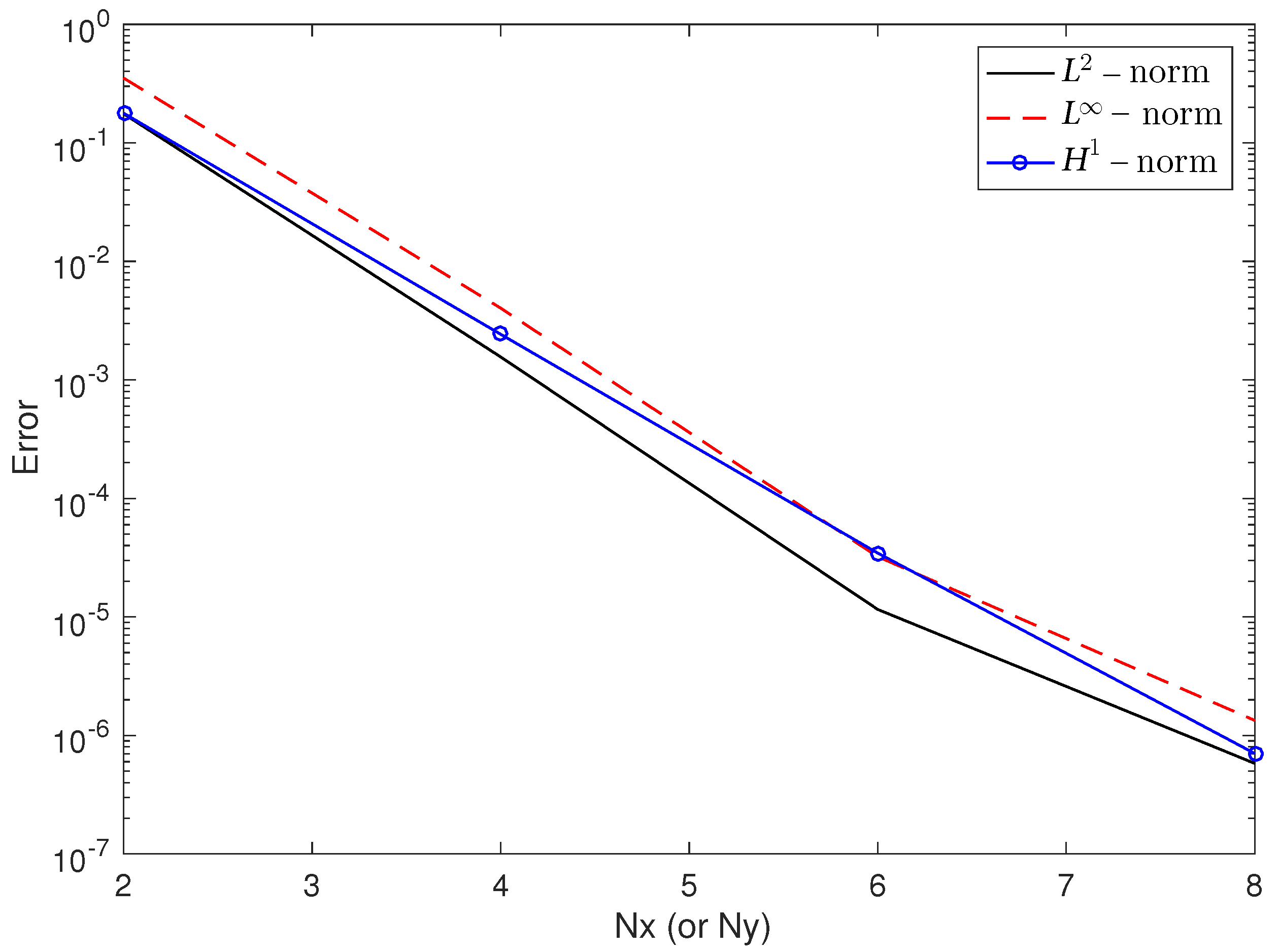
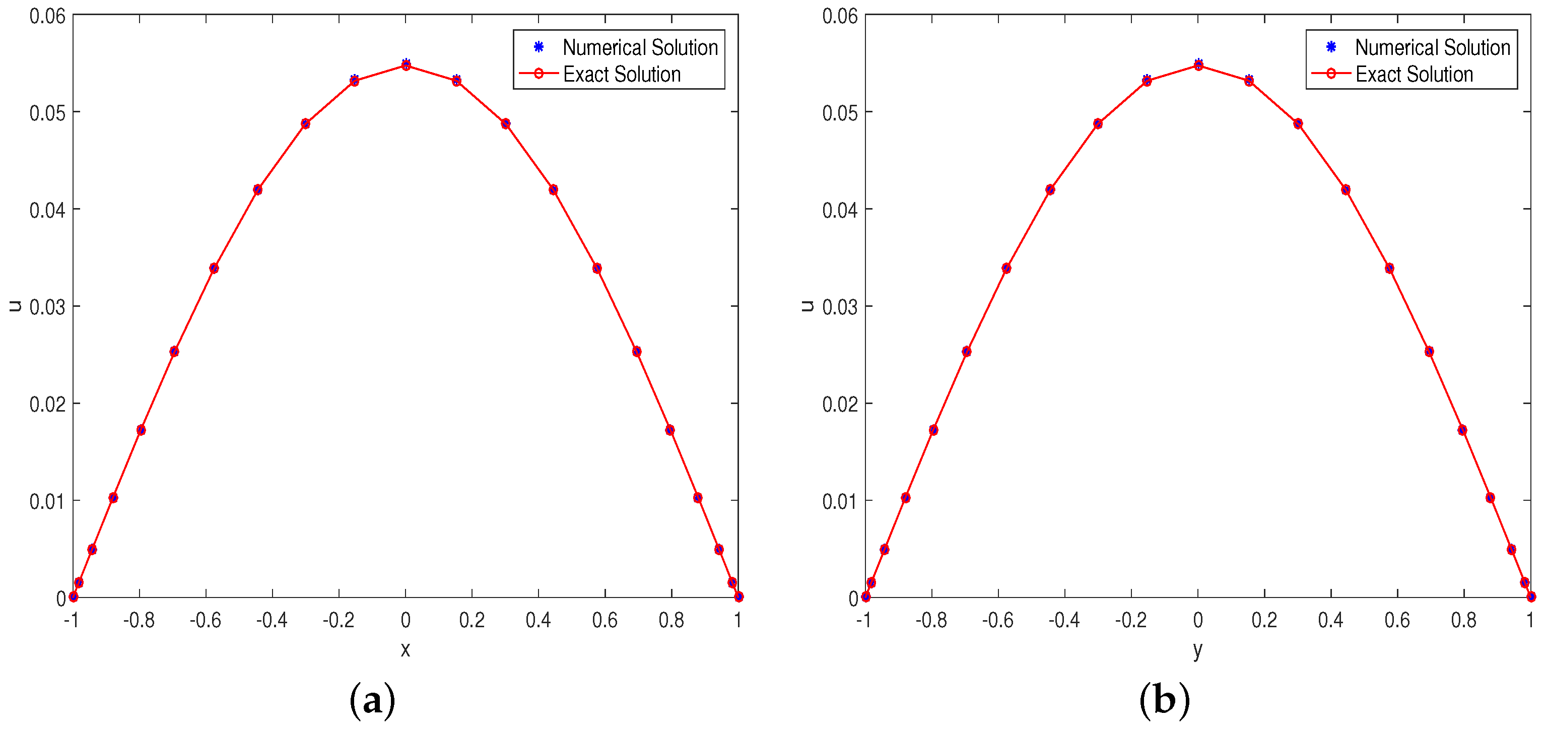
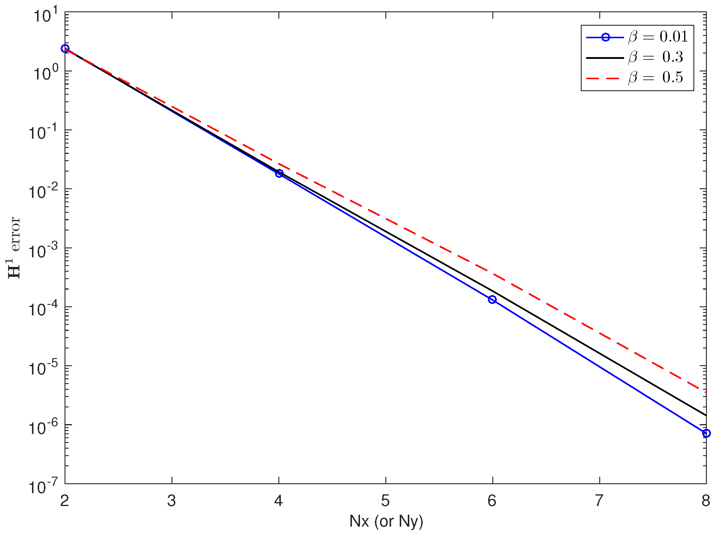
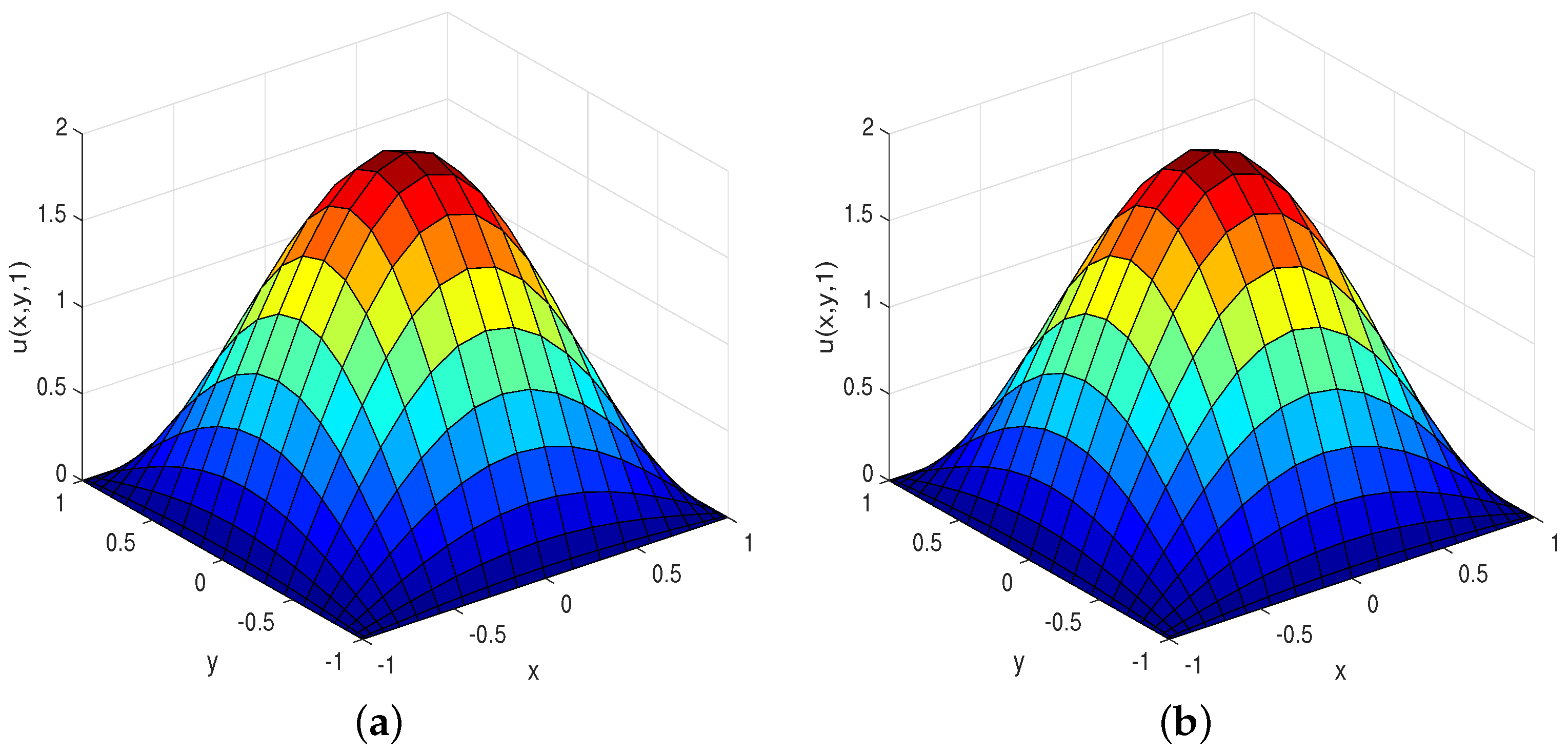
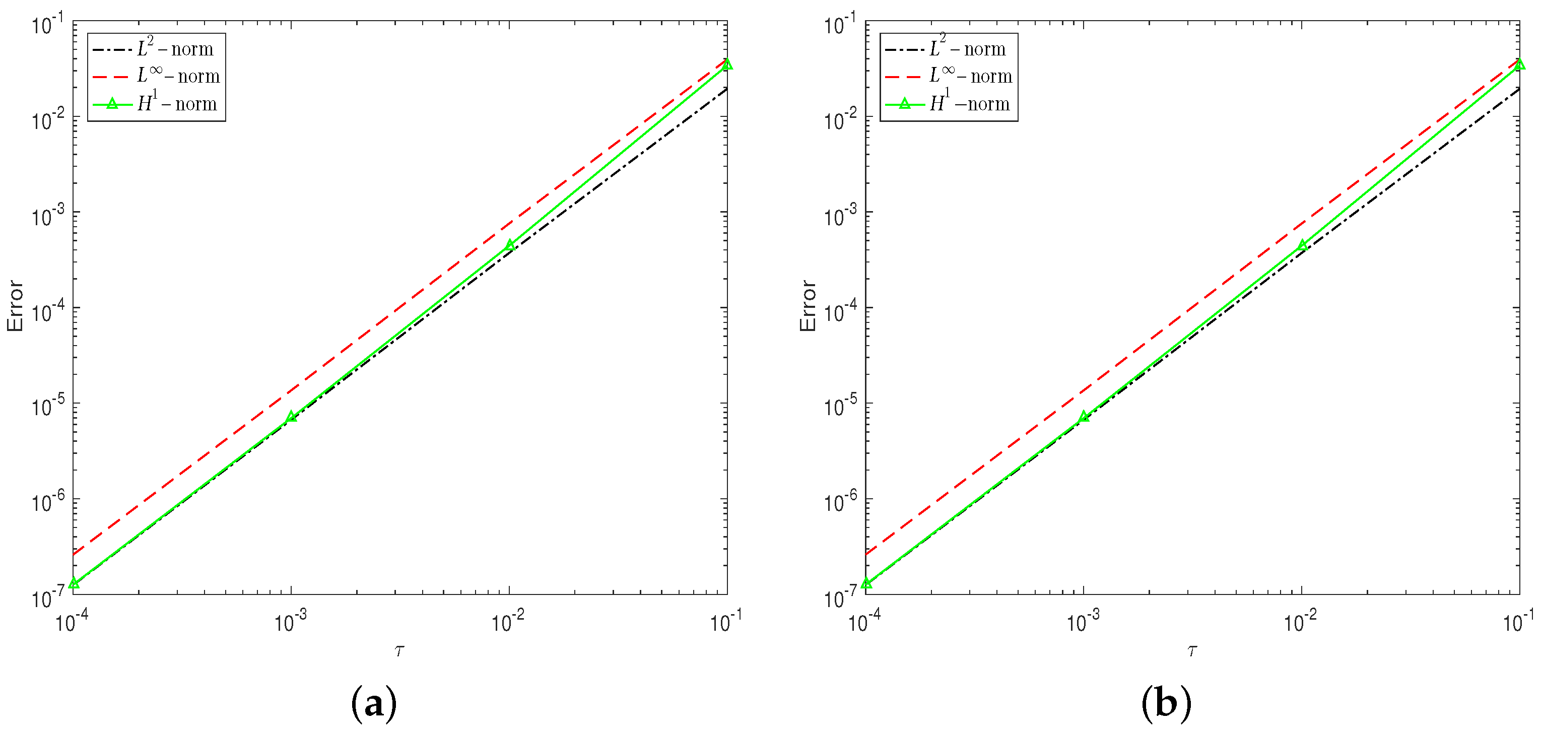
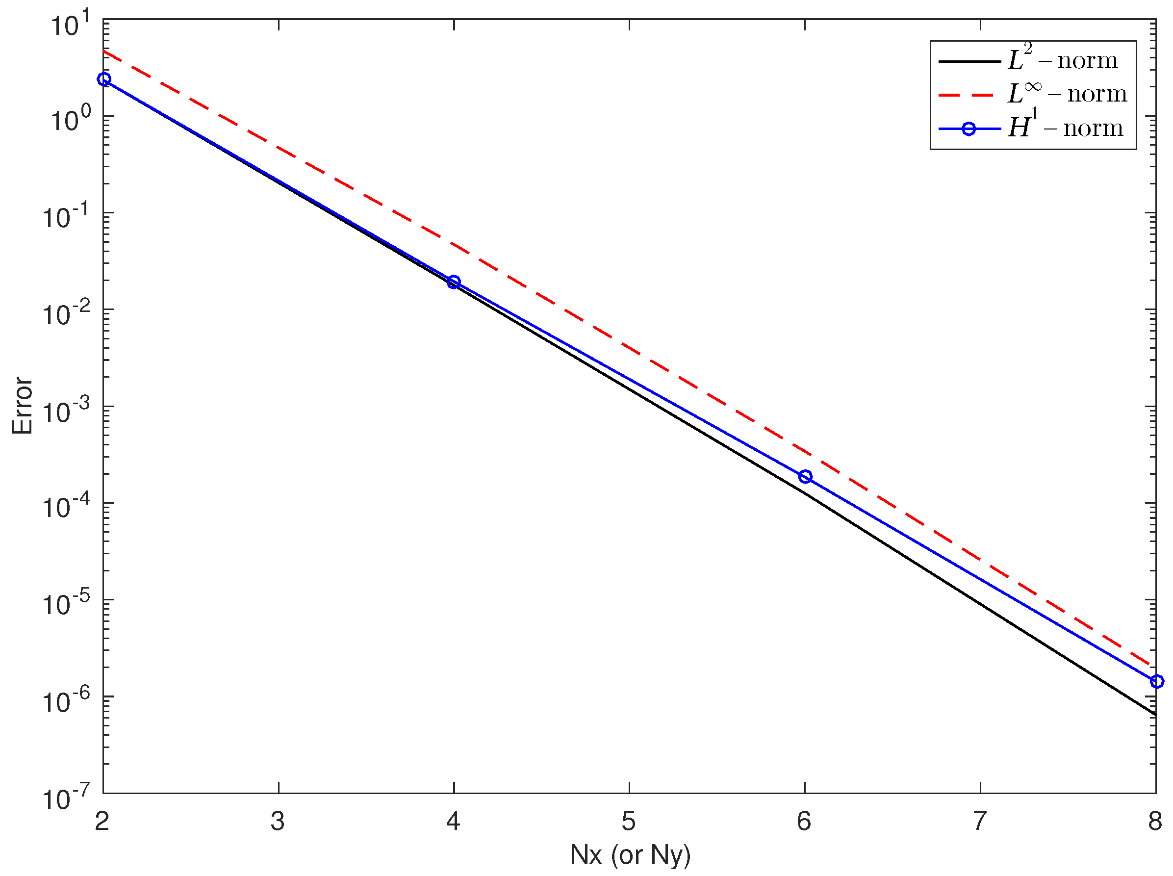
4. Numerical Results

In this section, we present numerical experiments to verify the theoretical analysis presented in Section 2. We shall consider two examples with homogeneous boundary conditions. To investigate the accuracy of the difference/spectral method, we compute the errors in three discrete norms, that is, $L^{\infty },L^2$, and $H^1$. The convergence order in time is defined as

$$\mathrm{order}\mathrm{in}\mathrm{time}=\frac{log\left(∥e({\tau }_2,N,t_k)∥/\phantom{∥e({\tau }_2,N,t_k)∥∥e({\tau }_1,N,t_k)∥}∥e({\tau }_1,N,t_k)∥\right)}{log\left({\tau }_2/\phantom{{\tau }_2{\tau }_1}{\tau }_1\right)},$$

(41)

where $e(\tau ,N,t_k)=u(x,y,t_k)-u_N^k,{\tau }_2\ne {\tau }_1.$

Example 1.

The 2D generalized time fractional cable equation:

$$\left\{\begin{array}{c}{\partial }_{t}u=-{}_0{D}_t^{\alpha }u+{}_0{D}_t^{\beta }\mathsf{\Delta }u+\mathsf{\Delta }u+f(x,y,t),x,y\in {(-1,1)}^2,t\in (0,1],\hfill \\ u(x,y,0)=sin\left(\frac{\pi }{2}x+\frac{\pi }{2}\right)sin\left(\frac{\pi }{2}y+\frac{\pi }{2}\right),x,y\in {[-1,1]}^2,\hfill \\ u(-1,y,t)=u(1,y,t)=0,t\in (0,1],y\in (-1,1),\hfill \\ u(x,-1,t)=u(x,1,t)=0,t\in (0,1],x\in (-1,1),\hfill \end{array}\right.$$

where

$$\begin{array}{c}f(x,y,t)=\left[\left(1+t^{3+\alpha +2\beta }\right)\frac{{\pi }^2}{2}+\left(3+\alpha +2\beta \right)t^{2+\alpha +2\beta }\right]sin\left(\frac{\pi }{2}x+\frac{\pi }{2}\right)sin\left(\frac{\pi }{2}y+\frac{\pi }{2}\right)\hfill \\ +\frac{{\pi }^2}{2}sin\left(\frac{\pi }{2}x+\frac{\pi }{2}\right)sin\left(\frac{\pi }{2}y+\frac{\pi }{2}\right)\{\frac{2t^{-\alpha }}{\mathsf{\Gamma }(1-\alpha ){\pi }^2}+\frac{t^{-\beta }}{\mathsf{\Gamma }(1-\beta )}\hfill \\ +\mathsf{\Gamma }\left(4+\alpha +2\beta \right)\left(\frac{2t^{3+2\beta }}{\mathsf{\Gamma }(4+2\beta ){\pi }^2}+\frac{{\mathrm{t}}^{3+\alpha +\beta }}{\mathsf{\Gamma }(4+\alpha +\beta )}\right)\}.\hfill \end{array}$$

The exact solution is $u(x,y,t)=\left(1+t^{3+\alpha +2\beta }\right)sin\left(\frac{\pi }{2}x+\frac{\pi }{2}\right)sin\left(\frac{\pi }{2}y+\frac{\pi }{2}\right).$

We first consider the temporal errors.

Table 1. The $L^{\infty },L^2,H^1-$ errors in time for three groups of $(\alpha ,\beta )$ at $N_x=N_y=8$.

$(\mathit{\alpha },\mathit{\beta })$	$\mathit{\tau }$	${\mathit{L}}^{\mathit{\infty }}$-Error	Order	${\mathit{L}}^2$-Error	Order	${\mathit{H}}^1$-Error	Order
$(0.1,0.9)$	1/40	$2.7896\times {10}^{-2}$		$1.3632\times {10}^{-2}$		$3.8184\times {10}^{-2}$
	1/80	$1.2995\times {10}^{-2}$	$1.1021$	$6.3503\times {10}^{-3}$	$1.1021$	$1.7225\times {10}^{-2}$	$1.1485$
	1/160	$6.0591\times {10}^{-3}$	$1.1008$	$2.9609\times {10}^{-3}$	$1.1008$	$7.7868\times {10}^{-3}$	$1.1454$
	1/320	$2.8263\times {10}^{-3}$	$1.1002$	$1.3811\times {10}^{-3}$	$1.1002$	$3.5244\times {10}^{-3}$	$1.1436$
	1/640	$1.3186\times {10}^{-3}$	$1.1000$	$6.4428\times {10}^{-4}$	$1.1000$	$1.5965\times {10}^{-3}$	$1.1425$
$(0.3,0.7)$	1/40	$1.1014\times {10}^{-2}$		$5.3823\times {10}^{-3}$		$1.1542\times {10}^{-2}$
	1/80	$4.4653\times {10}^{-3}$	$1.3025$	$2.1820\times {10}^{-3}$	$1.3026$	$4.3038\times {10}^{-3}$	$1.4232$
	1/160	$1.8096\times {10}^{-3}$	$1.3030$	$8.8427\times {10}^{-4}$	$1.3031$	$1.6132\times {10}^{-3}$	$1.4157$
	1/320	$7.3352\times {10}^{-4}$	$1.3028$	$3.5838\times {10}^{-4}$	$1.3030$	$6.0818\times {10}^{-4}$	$1.4074$
	1/640	$2.9746\times {10}^{-4}$	$1.3022$	$1.4528\times {10}^{-4}$	$1.3026$	$2.3071\times {10}^{-4}$	$1.3984$
$(0.5,0.5)$	1/40	$4.6711\times {10}^{-3}$		$2.2826\times {10}^{-3}$		$3.9660\times {10}^{-3}$
	1/80	$1.6554\times {10}^{-3}$	$1.4966$	$8.0887\times {10}^{-4}$	$1.4967$	$1.2604\times {10}^{-3}$	$1.6538$
	1/160	$5.8555\times {10}^{-4}$	$1.4993$	$2.8607\times {10}^{-4}$	$1.4995$	$4.0562\times {10}^{-4}$	$1.6356$
	1/320	$2.0705\times {10}^{-4}$	$1.4998$	$1.0110\times {10}^{-4}$	$1.5005$	$1.3244\times {10}^{-4}$	$1.6148$
	1/640	$7.3265\times {10}^{-5}$	$1.4988$	$3.5726\times {10}^{-5}$	$1.5008$	$4.3893\times {10}^{-5}$	$1.5933$

displays the relationship of $L^{\infty },L^2$ and $H^1$ errors with $(\alpha ,\beta )=(0.1,0.9),(0.3,0.7),(0.5,0.5),N_x=N_y=8,T=1$ for different step sizes $\tau$. We can observe that the convergence orders in time are approximately equal to $1.1(\alpha =0.1,\beta =0.9),1.3(\alpha =0.3,\beta =0.7),$ and $1.5(\alpha =0.5,\beta =0.5)$, which are in agreement with the theoretical analysis min{$2-\alpha ,2-\beta$}.

Next, we investigate the spatial errors. We fix a large enough value of $\tau ={10}^{-4}$, and let N vary. In Figure 1, we plot the errors as functions for the degree of the polynomials $N_x,N_y$ with $(\alpha ,\beta )=(0.5,0.5),T=1.$ We can obviously observe that the convergence in space of the present method is exponential.

Finally, we analyze the relationship between the numerical results and the exact solutions. Figure 2 shows the velocity distribution of the exact solution and the numerical solution by using the difference/spectral method with $\tau =0.01,N_x=N_y=20,\alpha =0.3,\beta =0.7,T=1.$ Then, the comparison between the numerical solution and the exact solution in the x direction with $y=0$ and in y direction with $x=0$ both at $\tau =0.01,N_x=N_y=20,\alpha =0.3,\beta =0.7,T=1$ is presented in Figure 3. It can be seen that our numerical results are very consistent with the exact solutions.

Example 2.

The 2D Rayleigh–Stokes problem for a heated generalized second-grade fluid with fractional derivatives:

$$\left\{\begin{array}{c}\partial u_t={}_0{D}_t^{\beta }\mathsf{\Delta }u+\mathsf{\Delta }u+f(x,y,t),x,y\in {(-1,1)}^2,t\in (0,1],\hfill \\ u(x,y,0)=20sin(\frac{\pi }{2}x+\frac{\pi }{2})sin(\frac{\pi }{2}y+\frac{\pi }{2}),x,y\in {[-1,1]}^2,\hfill \\ u(-1,y,t)=u(1,y,t)=0,t\in (0,1],y\in (-1,1),\hfill \\ u(x,-1,t)=u(x,1,t)=0,t\in (0,1],x\in (-1,1),\hfill \end{array}\right.$$

where

$$\begin{array}{c}f(x,y,t)=(6+\beta )t^{5+\beta }sin(\frac{\pi }{2}x+\frac{\pi }{2})sin(\frac{\pi }{2}y+\frac{\pi }{2})\hfill \\ +{\pi }^{2}sin(\frac{\pi }{2}x+\frac{\pi }{2})sin(\frac{\pi }{2}y+\frac{\pi }{2})\left\{(10+\frac{1}{2}{t}^{6+\beta })+\frac{10t^{-\beta }}{\mathsf{\Gamma }(1-\beta )}+\frac{\mathsf{\Gamma }(7+\beta )t^6}{1440}\right\}.\hfill \end{array}$$

The exact solution is $u(x,y,t)=(20+t^{6+\beta })sin(\frac{\pi }{2}x+\frac{\pi }{2})sin(\frac{\pi }{2}y+\frac{\pi }{2}).$

We first consider the temporal errors. We take $N_x=N_y=10$ so that the spatial discretization errors are negligible compared with the temporal errors. In Figure 4, we plot errors as functions of the time step $\tau$ for $\beta =0.01,0.3,$ and the slope of the error lines in this log-log plot also represents the convergence order in time. Secondly, we investigate the spatial errors. For a similar reason to the one mentioned above, we fix a large enough value of $\tau ={10}^{-4}$, and let N vary. In Figure 5 and Figure 6, we plot the errors as functions for the degree of polynomials $N_x,N_y$ with $\beta =0.3,T=1$ and $\beta =0.01,0.3,0.5,T=1.$ We can obviously observe that the convergence in space of the present method is exponential. Moreover, we find that the error decreases as the fractional derivative decreases. The numerical results are in agreement with the theoretical analysis.

5. Conclusions

In this study, we investigated a highly accurate numerical method for the 2D generalized time fractional cable equation by combining the second-order backward difference method in temporal discretization and the Galerkin spectral method in spatial discretization. We have proven that the scheme is unconditionally stable and have analyzed the error bounds of the present method. However, the limitation of accuracy in time causes a low global convergence rate. The difference/spectral method was proven to have $\min \{2-\alpha ,2-\beta \}$-order convergence in time and spectral accuracy in space for smooth solutions, where $\alpha ,\beta$ are two exponents of fractional derivatives. The numerical results confirmed the theoretical analysis and the high efficiency of the presented scheme. In this study we have thus developed an efficient numerical method which can be applied to model diffusion and viscoelastic non-Newtonian fluid flow.

References

1. Cui, M.R. Compact finite difference method for the fractional diffusion equation. J. Comput. Phys. 2009, 228, 7792–7804. [Google Scholar] [CrossRef]
2. Miller, K.S.; Ross, B. An Introduction to the Fractional Calculus and Fractional Differential Equations; John Wily and Sons Inc.: New York, NY, USA, 1993. [Google Scholar]
3. Metzler, R.; Klafter, J. The restaurant at the end of the random walk: Recent developments in the description of anomalous transport by fractional dynamics. J. Phys. A Math. Gen. 2004, 37, R161–R208. [Google Scholar] [CrossRef]
4. Podlubny, I. Geometric and physical interpretation of fractional integration and fractional differentiation. Fract. Calc. Appl. Anal. 2002, 5, 367–386. [Google Scholar]
5. Huang, J.F.; Nie, N.M.; Tang, Y.F. A second order finite difference-spectral method for space fractional diffusion equations. Sci. China Math. 2014, 57, 1303–1317. [Google Scholar] [CrossRef]
6. Henry, B.I.; Langlands, T.A.M.; Wearne, S.L. Fractional cable models for spiny neuronal dendrites. Phys. Rev. Lett. 2008, 100, 128103. [Google Scholar] [CrossRef]
7. Lin, Y.M.; Li, X.J.; Xu, C.J. Finite difference/spectral approximations for the fractional cable equation. Math. Comp. 2009, 80, 1369–1396. [Google Scholar] [CrossRef]
8. Langlands, T.A.M.; Henry, B.I.; Wearne, S.L. Fractional cable equation models for anomalous electrodiffusion in nerve cells: Infinite domain solutions. J. Math. Biol. 2009, 59, 761–808. [Google Scholar] [CrossRef]
9. Bazhlekova, E.; Jin, B.; Lazarov, R.; Zhou, Z. An analysis of the Rayleigh-Stokes problem for a generalized second-grade fluid. Numer. Math. 2015, 131, 1–31. [Google Scholar] [CrossRef]
10. Chen, C.M.; Liu, F.; Anh, V. A Fourier method and an extrapolation technique for Stokes’ first problem for a heated generalized second grade fluid with fractional derivative. J. Comput. Appl. Math. 2009, 223, 777–789. [Google Scholar] [CrossRef]
11. Huang, J.F.; Yang, D.D. A unified difference-spectral method for time-space fractional diffusion equations. Int. J. Comput. Math. 2017, 94, 1172–1184. [Google Scholar] [CrossRef]
12. Shen, F.; Tan, W.C.; Zhao, Y.H.; Masuoka, T. The Rayleigh-Stokes problem for a heated generalized second grade fluid with fractional derivative model. Nonlinear Anal. RWA 2006, 7, 1072–1080. [Google Scholar] [CrossRef]
13. Fetecau, C.; Fetecau, C. The first problem of Stokes for an Oldroyd-B fluid. Int. J. Non-Linear Mech. 2003, 38, 1539–1544. [Google Scholar] [CrossRef]
14. Tan, W.C.; Masuoka, T. Stokes’ first problem for a second grade fluid in a porous half-space with heated boundary. Int. J. Non-Linear Mech. 2005, 40, 515–522. [Google Scholar] [CrossRef]
15. Akyildiz, F.T. Stokes’ first problem for a Newtonian fluid in a non-Darcian porous half-space using a Laguerre-Galerkin method. Math. Methods Appl. Sci. 2007, 30, 2263–2277. [Google Scholar] [CrossRef]
16. Yu, B.; Jiang, X.Y. Numerical identification of the fractional derivatives in the two-dimensional fractional cable equation. J. Sci. Comput. 2016, 68, 252–272. [Google Scholar] [CrossRef]
17. Liu, Y.; Du, Y.W.; Li, H.; Wang, J.F. A two-grid finite element approximation for a nonlinear time-fractional Cable equation. Nonlinear Dyn. 2016, 85, 2535–2548. [Google Scholar] [CrossRef]
18. Zhang, H.X.; Yang, X.H.; Han, X.L. Discrete-time orthogonal spline collocation method with application to two-dimensional fractional cable equation. Comput. Math. Appl. 2014, 68, 1710–1722. [Google Scholar] [CrossRef]
19. Bhrawy, A.H.; Zaky, M.A. Numerical simulation for two-dimensional variable-order fractional nonlinear cable equation. Nonlinear Dyn. 2015, 80, 101–116. [Google Scholar] [CrossRef]
20. Dehghan, M.; Abbaszadeh, M. Analysis of the element free Galerkin (EFG) method for solving fractional cable equation with Dirichlet boundary condition. Appl. Numer. Math. 2016, 109, 208–234. [Google Scholar] [CrossRef]
21. Chen, C.M.; Liu, F.W.; Anh, V. Numerical analysis of the Rayleigh-Stokes problem for a heated generalized second grade fluid with fractional derivatives. Appl. Math. Comput. 2008, 204, 340–351. [Google Scholar] [CrossRef]
22. Mohebbi, A.; Abbaszadeh, M.; Dehghan, M. Compact finite difference scheme and RBF meshless approach for solving 2D Rayleigh-Stokes problem for a heated generalized second grade fluid with fractional derivatives. Comput. Methods Appl. Mech. Eng. 2013, 264, 163–177. [Google Scholar] [CrossRef]
23. Dehghan, M.; Abbaszadeh, M. A finite element method for the numerical solution of Rayleigh-Stokes problem for a heated generalized second grade fluid with fractional derivatives. Eng. Comput. Ger. 2017, 33, 587–605. [Google Scholar] [CrossRef]
24. Abdelkawy, M.A.; Alqahtani, R.T. Shifted Jacobi collocation method for solving multi-dimensional fractional Stokes’ first problem for a heated generalized second grade fluid. Adv. Differ. Equ. 2016, 2016, 114. [Google Scholar] [CrossRef]
25. Naz, A.; Ali, U.; Elfasakhany, A.; Ismail, K.A.; Al-Sehemi, A.G.; Al-Ghamdi, A.A. An implicit numerical approach for 2D Rayleigh Stokes problem for a heated generalized second grade fluid with fractional derivative. Fractal Fract. 2021, 5, 283. [Google Scholar] [CrossRef]
26. Langlands, T.A.M.; Henry, B.I.; Wearne, S.L. Fractional cable equation models for anomalous electrodiffusion in nerve cells: Finite domain solutions. SIAM J. Appl. Math. 2011, 71, 1168–1203. [Google Scholar] [CrossRef]
27. Li, C.; Deng, W.H. Analytical solutions, moments, and their asymptotic behaviors for the time-space fractional cable equation. Commun. Theor. Phys. 2014, 62, 54. [Google Scholar] [CrossRef]
28. Liu, F.W.; Chen, Y.Q.; Turner, I. Two new implicit numerical methods for the fractional cable equation. J. Comput. Nonlinear Dyn. 2011, 6, 0110091–0110097. [Google Scholar] [CrossRef]
29. Hu, X.L.; Zhang, L.M. Implicit compact difference schemes for the fractional cable equation. Appl. Math. Model. 2012, 36, 4027–4043. [Google Scholar] [CrossRef]
30. Chen, C.M.; Liu, F.W. Burrage, K. Numerical analysis for a variable-order nonlinear cable equation. J. Comput. Appl. Math. 2011, 236, 209–224. [Google Scholar] [CrossRef]
31. Zhuang, P.; Liu, F.; Turner, I.; Anh, V. Galerkin finite element method and error analysis for the fractional cable equation. Numer. Algorithms 2016, 72, 447–466. [Google Scholar] [CrossRef]
32. Nazar, M.; Fetecau, C.; Awan, A.U. A note on the unsteady flow of a generalized second-grade fluid through a circular cylinder subject to a time dependent shear stress. Nonlinear Anal. RWA 2010, 11, 2207–2214. [Google Scholar] [CrossRef]
33. Lin, Y.Z.; Jiang, W. Numerical method for Stokes’ first problem for a heated generalized second grade fluid with fractional derivative. Numer. Methods Partial. Differ. Equ. 2011, 27, 1599–1609. [Google Scholar] [CrossRef]
34. Podlubny, I. Fractional Differential Equations; Academic Press: New York, NY, USA, 1999. [Google Scholar]
35. Shen, J.; Tang, T. Spectral and High-Order Methods with Applications; Science Press: Beijing, China, 2006. [Google Scholar]
36. Shen, J.; Tang, T.; Wang, L.L. Spectral Methods: Algorithms, Analysis and Applications; Springer Science: Berlin/Heidelberg, Germany, 2011. [Google Scholar]
37. Trefethen, L.N. Spectral Methods in MATLAB; SIAM: Philadelphia, PA, USA, 2000. [Google Scholar]
38. Demmel, J.W. Applied Numerical Linear Algebra; SIAM: Philadelphia, PA, USA, 1997. [Google Scholar]
39. Hesthaven, J.S.; Gottlieb, S.; Gottlieb, D. Spectral Methods for Time-Dependent Problems; Cambridge University Press: Cambridge, UK, 2007. [Google Scholar]
40. Guo, B.Y. Spectral Methods and Their Applications; World Scientific: Singapore, 1998. [Google Scholar]
41. Li, X.J.; Xu, C.J. A space-time spectral method for the time fractional diffusion equation. SIAM J. Numer. Anal. 2009, 47, 2108–2131. [Google Scholar] [CrossRef]
42. Zeng, F.H.; Liu, F.W.; Li, C.P.; Burrage, K.; Turner, I.; Anh, V. A Crank-Nicolson ADI spectral method for a two-dimensional Riesz space fractional nonlinear reaction-diffusion equation. SIAM J. Numer. Anal. 2014, 52, 2599–2622. [Google Scholar] [CrossRef]
43. Zheng, M.L.; Liu, F.W.; Turner, I.; Anh, V. A novel high order space-time spectral method for the time fractional Fokker-Planck equation. SIAM J. Sci. Comput. 2015, 37, A701–A724. [Google Scholar] [CrossRef]
44. Lin, Y.M.; Xu, C.J. Finite difference/spectral approximation for the time fractional diffusion equations. J. Comput. Phys. 2007, 2, 1533–1552. [Google Scholar] [CrossRef]
45. Zheng, M.; Liu, F.; Anh, V.; Turner, I. A high-order spectral method for the multi-term time-fractional diffusion equations. Appl. Math. Model. 2016, 40, 4970–4985. [Google Scholar] [CrossRef]
46. Lu, C.W.; Xu, C.J. Improved error estimates of a finite difference/spectral method for time-fractional diffusion equations. Int. J. Numer. Anal. Model. 2015, 12, 384–400. [Google Scholar]
47. Bernardi, C.; Maday, Y. Approximations Spectrales de Problemes Aux Limites Elliptiques; Springer: Berlin/Heidelberg, Germany, 1992. [Google Scholar]
Figure 1. For α = 0.5 , β = 0.5 , τ = 0.0001 , T = 1 , the L , L 2 and H 1 errors show an exponential decay with N x , N y .
Fractalfract 06 00439 g001
Figure 2. The velocity distribution of the exact solution and the numerical solution with τ = 0.01 , N x = N y = 20 , α = 0.3 , β = 0.7 , T = 1 . (a) Exact result; (b) numerical result.
Fractalfract 06 00439 g002
Figure 3. Comparison between the numerical solution and the exact solution in two directions for τ = 0.01 , N x = N y = 20 , α = 0.3 , β = 0.7 , T = 1 . (a) x direction with y = 0 ; (b) y direction with x = 0 .
Fractalfract 06 00439 g003
Figure 4. For T = 1 , N x = N y = 10 and different β , the errors as a function of the time step τ . (a) β = 0.01 ; (b) β = 0.3 .
Fractalfract 06 00439 g004
Figure 5. For β = 0.3 , τ = 0.0001 , T = 1 , the L , L 2 and H 1 errors show an exponential decay with N x , N y .
Fractalfract 06 00439 g005
Figure 6. H 1 errors versus N x , N y when β = 0.01 , 0.3 , 0.5 .
Fractalfract 06 00439 g006