Article

A Fast High-Order Predictor–Corrector Method on Graded Meshes for Solving Fractional Differential Equations

1
School of Management Engineering, Qingdao University of Technology, Qingdao 266520, China
2
Applied and Computational Mathematics Division, Beijing Computational Science Research Center, Beijing 100193, China
*
Author to whom correspondence should be addressed.
Fractal Fract. 2022, 6(9), 516; https://doi.org/10.3390/fractalfract6090516
Submission received: 1 August 2022 / Revised: 28 August 2022 / Accepted: 7 September 2022 / Published: 13 September 2022

Abstract

:
In this paper, we focus on the computation of Caputo-type fractional differential equations. A high-order predictor–corrector method is derived by applying the quadratic interpolation polynomial approximation for the integral function. In order to deal with the weak singularity of the solution near the initial time of the fractional differential equations caused by the fractional derivative, graded meshes were used for time discretization. The error analysis of the predictor–corrector method is carefully investigated under suitable conditions on the data. Moreover, an efficient sum-of-exponentials (SOE) approximation to the kernel function was designed to reduce the computational cost. Lastly, several numerical examples are presented to support our theoretical analysis.

1. Introduction

Growing interest has focused on the study of fractional differential equations (FDEs) over the last few decades; see [1,2] and the references therein. Obtaining the exact solutions for FDEs can be very challenging, especially for general right-hand-side functions. Thus, there is a need to develop numerical methods for FDEs, for which extensive work has been conducted. One idea is to directly approximate the fractional derivative operators, e.g., [3,4,5]. Another idea is first to transform the FDEs into the integral forms and then use the numerical schemes to solve the integral equation; see, e.g., [6,7,8,9,10,11,12,13,14,15]. There are also some other numerical methods for FDEs, such as the variational iteration [16], Adomian decomposition [17], finite-element [18], and spectral [19] methods.
Adams methods are one of the most studied implicit–explicit linear multistep method groups. They play a major rule in the numerical processing of various differential equations. Therefore, great interest has been devoted to generalizing Adams methods to FDEs, especially the Adams-type predictor–corrector method. For example, Diethelm et al. [7,8,9,10] suggested the numerical approximation of FDEs using the Adams-type predictor–corrector method on uniform meshes. Deng [20] apprehended the short memory principle of fractional calculus and further applied the Adams-type predictor–corrector method for the numerical solution of FDEs on uniform meshes. Nguyen and Jang [21] studied a new Adams-type predictor–corrector method on uniform meshes by introducing a new prediction stage which is the same accuracy order as that of the correction stage for solving FDEs. Zhou et al. [22] considered the fast second-order Adams-type predictor–corrector method on graded meshes to solve a nonlinear time-fractional Benjamin–Bona–Mahony–Burgers equation.
Solutions to FDEs typically exhibit weak singularity at the initial time. In order to handle such problems, several techniques were developed, such as using nonuniform grids to keep errors small near the singularity [5,12,13,23,24,25], or employing correction terms to recover theoretical accuracy [6,15,26,27], or choosing a simple change in variable to derive a new and equivalent time-rescaled FDE [28,29].
In this paper, our goals are to construct high-order numerical methods and deal with the singularity of the solution of FDEs. Motivated by the above research, we follow the predictor–corrector method proposed in [21] and apply graded meshes to solve the following FDEs
C D 0 α y ( t ) = f ( t , y ( t ) ) for α ( 0 , 1 ) , t ( 0 , T ] ; y ( 0 ) = y 0 ,
where y 0 is a real number; C D 0 α denotes the fractional derivative in the Caputo sense, which is defined for all functions w that are absolutely continuous on t > 0 by (e.g., [1])
C D 0 α w ( t ) : = 1 Γ ( 1 α ) s = 0 t ( t s ) α w ( s ) d s for α ( 0 , 1 ) .
To ensure that the existence and uniqueness of the solution of Problem (1) (e.g., [8], Theorems 2.1, 2.2), we assumed that the continuous function f fulfilled the Lipschitz condition with respect to its second argument on a suitable set G, i.e., for any y , y ^ G ,
| f ( t , y ) f ( t , y ^ ) | L | y y ^ | for t [ 0 , T ] ,
where L > 0 is the Lipschitz constant independent of t , y and y ^ . Equation (1) can be rewritten as the following Volterra integral equation (e.g., [8])
y ( t ) = y 0 + 1 Γ ( α ) s = 0 t ( t s ) α 1 f y ( s ) d s with f y ( t ) = f ( t , y ( t ) ) .
The following regularity assumptions on the solution are also used for our proposed method:
y C [ 0 , T ] C 3 ( 0 , T ] with | y ( k ) ( t ) | C ( 1 + t α k ) for k = 0 , 1 , 2 , 3 , t ( 0 , T ] .
Moreover, we can learn from ([30], Section 2) or ([10], Theorem 2.1) that the analytical solution of (1) can be written as the summation of the singular and the regular parts; see the following lemma where for each s R , s : = min n N : n s .
Lemma 1
([10], Theorem 2.1).
(a) 
Suppose that f C 2 ( G ) . Then, there exist some constants c 1 , c 2 , , c v ^ R and a function ψ C 1 [ 0 , T ] such that
y ( t ) = ψ ( t ) + v = 1 v ^ c v t v α with v ^ : = 1 / α 1 .
(b) 
Suppose that f C 3 ( G ) . Then, there exist some constants c 1 , c 2 , , c v ^ R , d 1 , d 2 , , d v ˜ R and a function ψ C 2 [ 0 , T ] , such that
y ( t ) = ψ ( t ) + v = 1 v ^ c v t v α + v = 1 v ˜ d v t 1 + v α with v ^ : = 2 / α 1 , v ˜ : = 1 / α 1 .
From the above lemma, when f C m ( G ) , m 2 , there are some constants c 1 , c 2 , , c v ^ R , such that
y ( t ) = c 1 t α + c 2 t 2 α + + c v ^ t v ^ α + smoother terms .
Then
C D 0 α y ( t ) = d 1 + d 2 t α + + d v ^ t ( v ^ 1 ) α + smoother terms ,
where d 1 , d 2 , , d v ^ R are some constants. Therefore, assumptions (5) are reasonable, and we can also obtain for z : = C D 0 α y that
z C [ 0 , T ] C 3 ( 0 , T ] , | z ( k ) ( t ) | C ( 1 + t α k ) for k = 0 , 1 , 2 , 3 , t ( 0 , T ] .
The computational work and storage of the predictor–corrector method still remain very high due to the nonlocality of the fractional derivatives. Therefore, fast methods to reduce computational cost and storage were also investigated. For example, on the basis of an efficient sum-of-exponentials (SOE) approximation for the kernel function t β 1 , Jiang et al. [31] introduced a fast evaluation of the Caputo fractional derivative on the interval [ Δ t , T ] with a uniform absolute error ϵ , where β ( 0 , 1 ) and Δ t is the time step size. One can also refer to [32,33,34,35]. In the present paper, we also use this SOE technique to construct the corresponding fast predictor–corrector method for (1).
The rest of this paper is organized as follows. In Section 2, we formulate the high-order predictor–corrector method for (1). In Section 3, we discuss the error estimates of the predictor–corrector method. In Section 4, we propose a fast algorithm for the presented predictor–corrector method. Several numerical examples are given in Section 5 to illustrate the computational flexibility and verify our error estimates of the used methods. A brief conclusion is given in Section 6.
Notation: In this paper, notation C is used to denote a generic positive constant that is always independent of mesh size, but may take different values at different occurrences.

2. High-Order Predictor–Corrector Method

In order to handle the weak singularity of the solution of (1), we consider the graded meshes
t n = T ( n / N ) r for n = 0 , 1 , , N , τ n = t n t n 1 for n = 1 , 2 , , N ,
where constant mesh grading r 1 is chosen by the user. One can obtain that
t n C N r n r and τ n = T N r [ n r ( n 1 ) r ] C N r n r 1 for n = 1 , 2 , , N .
The discretized version of (4) at t = t n + 1 is given as
y ( t n + 1 ) = y 0 + 1 Γ ( α ) j = 0 n s = t j t j + 1 ( t n + 1 s ) α 1 f y ( s ) d s .
To construct the high-order predictor–corrector method for (1), on each small interval [ t j , t j + 1 ] , we denote the linear interpolation polynomial and quadratic interpolation polynomial of a function w ( t ) as Π 1 , j w ( t ) and Π 2 , j w ( t ) , respectively, i.e.,
Π 1 , j w ( t ) = t t j + 1 t j t j + 1 w ( t j ) + t t j t j + 1 t j w ( t j + 1 ) : = L j , 0 ( t ) w ( t j ) + L j , 1 ( t ) w ( t j + 1 ) for j = 0 , 1 , , N 1 ,
and
Π 2 , j w ( t ) = ( t t j ) ( t t j + 1 ) ( t j 1 t j ) ( t j 1 t j + 1 ) w ( t j 1 ) + ( t t j 1 ) ( t t j + 1 ) ( t j t j 1 ) ( t j t j + 1 ) w ( t j ) + ( t t j 1 ) ( t t j ) ( t j + 1 t j 1 ) ( t j + 1 t j ) w ( t j + 1 ) : = Q j , 1 ( t ) w ( t j 1 ) + Q j , 0 ( t ) w ( t j ) + Q j , 1 ( t ) w ( t j + 1 ) for j = 1 , 2 , , N 1 .
Set
a j , θ n + 1 : = s = t j t j + 1 ( t n + 1 s ) α 1 L j , θ ( s ) d s with θ = 0 or 1 , j = 0 , 1 , , n ,
b j , θ n + 1 : = s = t j t j + 1 ( t n + 1 s ) α 1 Q j , θ ( s ) d s with θ = 1 , 0 or 1 , j = 1 , 2 , , n ,
c j , θ n + 1 : = s = t j t j + 1 ( t n + 1 s ) α 1 Q j 1 , θ ( s ) d s with θ = 1 , 0 or 1 , j = 2 , 3 , , n .
For the calculation of the predictor formula of (8), we do not use the unknown value y ( t n + 1 ) when computing s = t n t n + 1 ( t n + 1 s ) α 1 f y ( s ) d s . Three cases are divided for n as follows:
  • When n = 0 , we use f y ( t 0 ) to approximate f y ( t ) on interval [ t 0 , t 1 ] .
  • When n = 1 , we use Π 1 , 0 f y ( t ) to approximate f y ( t ) on intervals [ t 0 , t 1 ] and [ t 1 , t 2 ] .
  • When n 2 , we use Π 1 , 0 f y ( t ) to approximate f y ( t ) on first small interval [ t 0 , t 1 ] , Π 2 , j f y ( t ) to approximate f y ( t ) on each interval [ t j , t j + 1 ] ( j = 1 , 2 , , n 1 ) and Π 2 , n 1 f y ( t ) to approximate f y ( t ) on the last small interval [ t n , t n + 1 ] .
Then, it follows from (8) that
y ( t n + 1 ) y 0 + 1 Γ ( α ) s = t 0 t 1 ( t n + 1 s ) α 1 Π 1 , 0 f y ( s ) d s + 1 Γ ( α ) j = 1 n 1 s = t j t j + 1 ( t n + 1 s ) α 1 Π 2 , j f y ( s ) d s + 1 Γ ( α ) s = t n t n + 1 ( t n + 1 s ) α 1 Π 2 , n 1 f y ( s ) d s = y 0 + 1 Γ ( α ) j = 0 n d j n + 1 f y ( t j ) + c n , 1 n + 1 f y ( t n 2 ) + c n , 0 n + 1 f y ( t n 1 ) + c n , 1 n + 1 f y ( t n ) ,
where Π 2 , 1 w ( t ) : = Π 1 , 0 w ( t ) + w ( t 0 ) , Π 2 , 0 w ( t ) : = Π 1 , 0 w ( t ) for a function w ( t ) , and
d 0 1 = 0 , c 0 , 1 1 = c 0 , 0 1 = 0 , c 0 , 1 1 = s = t 0 t 1 ( t 1 s ) α 1 d s ( for n = 0 ) ; d 0 2 = a 0 , 0 2 , d 1 2 = a 0 , 1 2 , c 1 , 1 2 = 0 ,
c 1 , θ 2 = s = t 1 t 2 ( t 2 s ) α 1 L 0 , θ ( s ) d s with θ = 0 or 1 ( for n = 1 ) ;
d 0 3 = a 0 , 0 3 + b 1 , 1 3 , d 1 3 = a 0 , 1 3 + b 1 , 0 3 , d 2 3 = b 1 , 1 3 ( for n = 2 ) ;
and, for n 3 ,
d j n + 1 = a 0 , 0 n + 1 + b 1 , 1 n + 1 , for j = 0 , a 0 , 1 n + 1 + b 1 , 0 n + 1 + b 2 , 1 n + 1 , for j = 1 , b j 1 , 1 n + 1 + b j , 0 n + 1 + b j + 1 , 1 n + 1 , for 2 j n 2 , b n 2 , 1 n + 1 + b n 1 , 0 n + 1 , for j = n 1 , b n 1 , 1 n + 1 , for j = n .
For the corrector formula of (8), we use Π 1 , 0 f y ( t ) to approximate f y ( t ) on the first small interval [ t 0 , t 1 ] , and Π 2 , j f y ( t ) to approximate f y ( t ) on intervals [ t j , t j + 1 ] ( j = 1 , 2 , , n ) . Hence, we can obtain from (8) that
y ( t n + 1 ) y 0 + 1 Γ ( α ) s = t 0 t 1 ( t n + 1 s ) α 1 Π 1 , 0 f y ( s ) d s + 1 Γ ( α ) j = 1 n s = t j t j + 1 ( t n + 1 s ) α 1 Π 2 , j f y ( s ) d s = y 0 + 1 Γ ( α ) j = 0 n d j n + 1 f y ( t j ) + b n , 1 n + 1 f y ( t n 1 ) + b n , 0 n + 1 f y ( t n ) + b n , 1 n + 1 f y ( t n + 1 ) ,
where
b 0 , 1 1 = 0 , b 0 , 0 1 = a 0 , 0 1 , b 0 , 1 1 = a 0 , 1 1 ( for n = 0 ) .
We denote the preliminary approximation of y ( t n + 1 ) from (12) as y n + 1 P (used in (15)) and the final approximation of y ( t n + 1 ) from (15) as y n + 1 . Then, with (12) and (15), our predictor–corrector method for Problem (1) can be derived as follows:
y n + 1 P = y 0 + 1 Γ ( α ) j = 0 n d j n + 1 f j + c n , 1 n + 1 f n 2 + c n , 0 n + 1 f n 1 + c n , 1 n + 1 f n , y n + 1 = y 0 + 1 Γ ( α ) j = 0 n d j n + 1 f j + b n , 1 n + 1 f n 1 + b n , 0 n + 1 f n + b n , 1 n + 1 f n + 1 P ,
where f j : = f ( t j , y j ) and f j P : = f ( t j , y j P ) .
Remark 1.
We use the same approximation of integral s = t 0 t n ( t n + 1 s ) α 1 f y ( s ) ds for the calculation of predictor Formula (12) and corrector Formula (15), which had the greatest computational burden. Thus, this reduces the overall cost of the predictor–corrector method. In addition, even though our predictor–corrector method (17) can be viewed as a generalization of the predictor–corrector method presented in [21], unlike their method, we did not need to use the values of y ( t 1 / 4 ) and y ( t 1 / 2 ) to start up the scheme.

3. Error Estimates of the Predictor–Corrector Method

In this section, we study the error analysis of the predictor–corrector method (17). For this, we first introduce some lemmas that are used in analysis.
Lemma 2
([11], Lemma 3.3). Assume that k j , n C τ j + 1 ( t n t j ) α 1 with 0 j n 1 , 1 n N . Let ψ 0 0 . Assume also that sequence ϕ n n = 0 N satisfies
ϕ 0 ψ 0 , ϕ n ψ 0 + j = 0 n 1 k j , n ϕ j for 1 n N .
Then, one has
ϕ n C ψ 0 for 1 n N .
Lemma 3.
Terms d j n + 1 , b j , 1 n + 1 , b j , 0 n + 1 , b j , 1 n + 1 and c j , 1 n + 1 , c j , 0 n + 1 , c j , 1 n + 1 in (11), (13), (14) and (16) satisfy the following estimates:
| d j n + 1 | C τ j + 1 ( t n + 1 t j ) α 1 for 0 j n , 0 n N 1 ,
| c n , 1 n + 1 | C τ n 1 ( t n + 1 t n 2 ) α 1 for 2 n N 1 ,
| c n , 0 n + 1 | , | b n , 1 n + 1 | C τ n ( t n + 1 t n 1 ) α 1 for 1 n N 1 ,
| c n , 1 n + 1 | , | b n , 0 n + 1 | , | b n , 1 n + 1 | C τ n + 1 α for 0 n N 1 .
Proof. 
A simple deduction from the expression of L j , θ ( θ = 0 or 1 ) and Q j , θ ( θ = 1 , 0 or 1 ) in (9) and (10) gives
| L j , θ | C for θ = 0 or 1 , | Q j , θ | C for θ = 1 , 0 or 1 .
Then, from (11), we have for 0 j n and θ = 0 or 1 that
| a j , θ n + 1 | C s = t j t j + 1 ( t n + 1 s ) α 1 d s C ( t n + 1 t j ) α ( t n + 1 t j + 1 ) α C τ j + 1 ( t n + 1 t j ) α 1 t n + 1 t j t n + 1 t j + 1 1 α C τ j + 1 ( t n + 1 t j ) α 1 1 + τ j + 1 τ n + 1 + τ n + + τ j + 2 1 α C τ j + 1 ( t n + 1 t j ) α 1 .
Again, one can obtain that
| b j , θ n + 1 | C τ j + 1 ( t n + 1 t j ) α 1 with θ = 1 , 1 or 1 , j = 0 , 1 , , n ,
| c j , θ n + 1 | C τ j + 1 ( t n + 1 t j ) α 1 with θ = 1 , 1 or 1 , j = 0 , 1 , , n .
Moreover,
τ j + 2 ( t n + 1 t j + 1 ) α 1 = τ j + 1 ( t n + 1 t j ) α 1 τ j + 2 τ j + 1 t n + 1 t j t n + 1 t j + 1 1 α C τ j + 1 ( t n + 1 t j ) α 1 τ 2 τ 1 1 + τ j + 1 τ n + 1 + τ n + + τ j + 2 1 α C τ j + 1 ( t n + 1 t j ) α 1 .
Hence, for 2 j n 2 , n 3 , one has from (14) that
| d j n + 1 | | b j 1 , 1 n + 1 | + | b j , 0 n + 1 | + | b j + 1 , 1 n + 1 | C τ j ( t n + 1 t j 1 ) α 1 + C τ j + 1 ( t n + 1 t j ) α 1 + C τ j + 2 ( t n + 1 t j + 1 ) α 1 C τ j + 1 ( t n + 1 t j ) α 1 .
Similar to the above inequalities, we can obtain other cases of the bound of | d j n + 1 | ; that is,
| d j n + 1 | C τ j + 1 ( t n + 1 t j ) α 1 for j = 0 , 1 , , n , n = 0 , 1 , , N 1 .
In addition, by using (18)–(20), we obtain
| c n , 1 n + 1 | C τ n + 1 ( t n + 1 t n ) α 1 C τ n ( t n + 1 t n 1 ) α 1 C τ n 1 ( t n + 1 t n 2 ) α 1 for 2 n N 1 ,
| c n , 0 n + 1 | , | b n , 1 n + 1 | C τ n + 1 ( t n + 1 t n ) α 1 C τ n ( t n + 1 t n 1 ) α 1 for 1 n N 1 ,
| c n , 1 n + 1 | , | b n , 0 n + 1 | , | b n , 1 n + 1 | C τ n + 1 α for 0 n N 1 .
Therefore, the proof is now completed. □
For r 1 and 0 < α < 1 . Define
Φ ( N , r , α ) : = N 2 r α for 1 r < 3 2 α , N 3 ln N for r = 3 2 α , N 3 for r > 3 2 α .
Lemma 4.
Let w C [ 0 , T ] C 3 ( 0 , T ] . Suppose that | w ( k ) ( t ) | C ( 1 + t α k ) for k = 0 , 1 , 2 , 3 , t ( 0 , T ] . For n 0 , we define
I 1 n + 1 = s = t 0 t 1 ( t n + 1 s ) α 1 ( w Π 1 , 0 w ) ( s ) d s + j = 1 n s = t j t j + 1 ( t n + 1 s ) α 1 ( w Π 2 , j w ) ( s ) d s ,
and
I 2 n + 1 = s = t 0 t 1 ( t n + 1 s ) α 1 ( w Π 1 , 0 w ) ( s ) d s + j = 1 n 1 s = t j t j + 1 ( t n + 1 s ) α 1 ( w Π 2 , j w ) ( s ) d s + s = t n t n + 1 ( t n + 1 s ) α 1 ( w Π 2 , n 1 w ) ( s ) d s .
Then, we have
I 1 n + 1 + I 2 n + 1 C Φ ( N , r , α ) for 0 n N 1 .
The proof of the above lemma is a bit lengthy. For the detailed proof, see Appendix A. Set
e j = y ( t j ) y j , e j P = y ( t j ) y j P for j = 0 , 1 , , N .
On the basis of the above preliminaries, a convergence criterion of the predictor–corrector method (17) can be stated as follows.
Theorem 1.
Suppose that y ( t j ) and y j j = 0 N are the solutions of (8) and (17), respectively. Suppose also that (5) holds true. Then, we have
| e j | C Φ ( N , r , α ) for 1 j N .
Proof. 
We can obtain from (8), (12), (15) and (17) that
e n + 1 P = 1 Γ ( α ) [ s = t 0 t 1 ( t n + 1 s ) α 1 ( f y Π 1 , 0 f y ) ( s ) d s + j = 1 n 1 s = t j t j + 1 ( t n + 1 s ) α 1 ( f y Π 2 , j f y ) ( s ) d s + s = t n t n + 1 ( t n + 1 s ) α 1 ( f y Π 2 , n 1 f y ) ( s ) d s ] + 1 Γ ( α ) [ j = 0 n d j n + 1 f y ( t j ) f j + c n , 1 n + 1 f y ( t n 2 ) f n 2 + c n , 0 n + 1 f y ( t n 1 ) f n 1 + c n , 1 n + 1 ( f y ( t n ) f n ) ] : = R 1 , 1 + R 1 , 2 ,
and
e n + 1 = 1 Γ ( α ) [ s = t 0 t 1 ( t n + 1 s ) α 1 ( f y Π 1 , 0 f y ) ( s ) d s + j = 1 n s = t j t j + 1 ( t n + 1 s ) α 1 ( f y Π 2 , j f y ) ( s ) d s ] + 1 Γ ( α ) j = 0 n d j n + 1 f y ( t j ) f j + b n , 1 n + 1 f y ( t n 1 ) f n 1 + b n , 0 n + 1 f y ( t n ) f n + 1 Γ ( α ) b n , 1 n + 1 f y ( t n + 1 ) f n + 1 P : = R 2 , 1 + R 2 , 2 + R 2 , 3 .
By using (1), (5), (6) and Lemma 4, we have
| R 1 , 1 | + | R 2 , 1 | C Φ ( N , r , α ) .
It follows from (3) and Lemma 3 that
| R 1 , 2 | C L j = 0 n | d j n + 1 | | e j | + C L | c n , 1 n + 1 | | e n 2 | + | c n , 0 n + 1 | | e n 1 | + | c n , 1 n + 1 | | e n | ,
| R 2 , 2 | C L j = 0 n | d j n + 1 | | e j | + C L ( | b n , 1 n + 1 | | e n 1 | + | b n , 0 n + 1 | | e n | ) ,
and
| R 2 , 3 | C L τ n + 1 α | e n + 1 P | .
Then, we obtain from (22)–(27) that
| e n + 1 P | C Φ ( N , r , α ) + C L j = 0 n | d j n + 1 | | e j | + C L | c n , 1 n + 1 | | e n 2 | + | c n , 0 n + 1 | | e n 1 | + | c n , 1 n + 1 | | e n | ,
and
| e n + 1 | C Φ ( N , r , α ) + C L j = 0 n | d j n + 1 | | e j | + C L | b n , 1 n + 1 | | e n 1 | + | b n , 0 n + 1 | | e n | + C L τ n + 1 α | e n + 1 P | .
Substituting (28) into (29) gives
| e n + 1 | C Φ ( N , r , α ) + C j = 0 n | d j n + 1 | | e j | + C | c n , 1 n + 1 | | e n 2 | + | c n , 0 n + 1 | | e n 1 | + | c n , 1 n + 1 | | e n | + C | b n , 1 n + 1 | | e n 1 | + | b n , 0 n + 1 | | e n | C 1 Φ ( N , r , α ) + C 1 j = 0 n τ j + 1 ( t n + 1 t j ) α 1 | e j |
for a fixed constant C 1 with the use of Lemma 3. Invoking Lemma 2 to (30) gives
| e n + 1 | C Φ ( N , r , α ) for 0 n N 1 .
The proof is, thus, complete. □
Remark 2.
Our predictor–corrector method (17) can easily be generalized to solve (1) with α 1 . The corresponding convergence order is
| e j | C N 3 ln N for 2 r α = 3 , N 3 otherwise , with 1 j N .

4. Construction of the Fast Algorithm

Due to the nonlocality of the fractional derivatives, our predictor–corrector method (17) also needed high computational work and storage. In order to overcome this difficulty, inspired by Jiang [31], in this section we consider the corresponding sum-of-exponentials (SOE) technique to improve the computational efficiency of the predictor–corrector method (17). Before deriving the fast predictor–corrector method, we give the following lemma for the SOE approximation.
Lemma 5
([31], Section 2.1). For the given β ( 0 , 2 ) , an absolute tolerance error ϵ, a cut-off time Δ t : = min 1 n N τ n and a final time T, there exist a positive integer N e x p , positive quadrature nodes s i , and corresponding positive weights ϖ i ( i = 1 , 2 , , N e x p ) such that
| t β i = 1 N e x p ϖ i e s i t | ϵ for t [ Δ t , T ] ,
where
N e x p = O log 1 ϵ log log 1 ϵ + log T Δ t + log 1 Δ t log log 1 ϵ + log 1 Δ t .
Now, we describe the fast predictor–corrector method, and we obtain from (12) that
y ( t n + 1 ) y 0 + 1 Γ ( α ) [ s = t 0 t 1 Π 1 , 0 f y ( s ) i = 1 N e x p ϖ i e s i ( t n + 1 s ) d s + j = 1 n 1 s = t j t j + 1 Π 2 , j f y ( s ) i = 1 N e x p ϖ i e s i ( t n + 1 s ) d s ] + 1 Γ ( α ) s = t n t n + 1 ( t n + 1 s ) α 1 Π 2 , n 1 f y ( s ) d s = y 0 + 1 Γ ( α ) i = 1 N e x p ϖ i [ s = t 0 t 1 e s i ( t n + 1 s ) Π 1 , 0 f y ( s ) d s + j = 1 n 1 s = t j t j + 1 e s i ( t n + 1 s ) Π 2 , j f y ( s ) d s ] + 1 Γ ( α ) s = t n t n + 1 ( t n + 1 s ) α 1 Π 2 , n 1 f y ( s ) d s = y 0 + 1 Γ ( α ) i = 1 N e x p ϖ i P i n + c n , 1 n + 1 f y ( t n 2 ) + c n , 0 n + 1 f y ( t n 1 ) + c n , 1 n + 1 f y ( t n ) ,
where P i 0 = 0 for i = 1 , 2 , , N e x p and
P i n = s = t 0 t 1 e s i ( t n + 1 s ) Π 1 , 0 f y ( s ) d s + j = 1 n 1 s = t j t j + 1 e s i ( t n + 1 s ) Π 2 , j f y ( s ) d s for i = 1 , 2 , , N e x p , n = 1 , 2 , , N 1 .
By using a recursive relation, one has that
P i n = s = t 0 t 1 e s i ( t n + τ n + 1 s ) Π 1 , 0 f y ( s ) d s + j = 1 n 2 s = t j t j + 1 e s i ( t n + τ n + 1 s ) Π 2 , j f y ( s ) d s + s = t n 1 t n e s i ( t n + 1 s ) Π 2 , n 1 f y ( s ) d s = e s i τ n + 1 s = t 0 t 1 e s i ( t n s ) Π 1 , 0 f y ( s ) d s + j = 1 n 2 s = t j t j + 1 e s i ( t n s ) Π 2 , j f y ( s ) d s + s = t n 1 t n e s i ( t n + 1 s ) Π 2 , n 1 f y ( s ) d s = e s i τ n + 1 P i n 1 + A i , 1 n + 1 f y ( t n 2 ) + A i , 0 n + 1 f y ( t n 1 ) + A i , 1 n + 1 f y ( t n ) for n = 2 , 3 , , N 1 ,
where
A i , θ n + 1 : = s = t n 1 t n e s i ( t n + 1 s ) Q n 1 , θ ( s ) d s with θ = 1 , 0 or 1 , n = 2 , 3 , , N 1 .
Similarly, we have from (15) that
y ( t n + 1 ) y 0 + 1 Γ ( α ) i = 1 N e x p ϖ i P i n + b n , 1 n + 1 f y ( t n 1 ) + b n , 0 n + 1 f y ( t n ) + b n , 1 n + 1 f y ( t n + 1 ) .
The prediction and correction stages approximations of y ( t n + 1 ) are denoted with y ¯ n + 1 P and y ¯ n + 1 , respectively. Set f ¯ j = f ( t j , y ¯ j ) and f ¯ j P : = f ( t j , y ¯ j P ) . Then, we obtain the fast predictor–corrector method for Problem (1) from (31)–(33):
y ¯ n + 1 P = y 0 + 1 Γ ( α ) i = 1 N e x p ϖ i p ¯ i n + c n , 1 n + 1 f ¯ n 2 + c n , 0 n + 1 f ¯ n 1 + c n , 1 n + 1 f ¯ n , y ¯ n + 1 = y 0 + 1 Γ ( α ) i = 1 N e x p ϖ i p ¯ i n + b n , 1 n + 1 f ¯ n 1 + b n , 0 n + 1 f ¯ n + b n , 1 n + 1 f ¯ n + 1 P , p ¯ i 0 = 0 , p ¯ i 1 = s = t 0 t 1 e s i ( t n + 1 s ) ( L 0 , 0 f ¯ 0 + L 0 , 1 f ¯ 1 ) d s for i = 1 , 2 , , N e x p , p ¯ i n = e s i τ n + 1 p ¯ i n 1 + A i , 1 n + 1 f ¯ n 2 + A i , 0 n + 1 f ¯ n 1 + A i , 1 n + 1 f ¯ n for i = 1 , 2 , , N e x p , n = 2 , 3 , , N .
The next result is the fundamental convergence bound for our fast predictor–corrector method (34).
Lemma 6.
Let w C [ 0 , T ] C 3 ( 0 , T ] . Suppose that | w ( k ) ( t ) | C ( 1 + t α k ) for k = 0 , 1 , 2 , 3 , t ( 0 , T ] . For n 0 , we define
I 3 n + 1 = | s = t 0 t n + 1 ( t n + 1 s ) α 1 w ( s ) d s s = t 0 t 1 Π 1 , 0 w ( s ) i = 1 N e x p ϖ i e s i ( t n + 1 s ) d s j = 1 n 1 s = t j t j + 1 Π 2 , j w ( s ) i = 1 N e x p ϖ i e s i ( t n + 1 s ) d s s = t n t n + 1 ( t n + 1 s ) α 1 Π 2 , n w ( s ) d s |
and
I 4 n + 1 = | s = t 0 t n + 1 ( t n + 1 s ) α 1 w ( s ) d s s = t 0 t 1 Π 1 , 0 w ( s ) i = 1 N e x p ϖ i e s i ( t n + 1 s ) d s j = 1 n 1 s = t j t j + 1 Π 2 , j w ( s ) i = 1 N e x p ϖ i e s i ( t n + 1 s ) d s s = t n t n + 1 ( t n + 1 s ) α 1 Π 2 , n 1 w ( s ) d s | .
Then, we have
I 3 n + 1 + I 4 n + 1 C Φ ( N , r , α ) + C ϵ for 0 n N 1 .
Proof. 
We can obtain that
I 3 n + 1 I 1 n + 1 + | s = t 0 t 1 Π 1 , 0 w ( s ) ( t n + 1 s ) α 1 i = 1 N e x p ϖ i e s i ( t n + 1 s ) d s + j = 1 n 1 s = t j t j + 1 Π 2 , j w ( s ) ( t n + 1 s ) α 1 i = 1 N e x p ϖ i e s i ( t n + 1 s ) d s d s | I 1 n + 1 + ϵ | s = t 0 t 1 Π 1 , 0 w ( s ) d s + j = 1 n 1 s = t j t j + 1 Π 2 , j w ( s ) d s | I 1 n + 1 + C ϵ t n max t 0 t t n | w ( t ) | C Φ ( N , r , α ) + C ϵ ,
where we used Lemmas 4 and 5. The proof of the bound of I 4 n + 1 is similar. □
The following theorem can easily be obtained by repeating the proof of Theorem 1.
Theorem 2.
Suppose that y ( t j ) and y ¯ j j = 0 N are the solutions of (8) and (34), respectively. Suppose also that (5) holds true. Then, we have
| y ( t j ) y ¯ j | C Φ ( N , r , α ) + C ϵ for 1 j N .

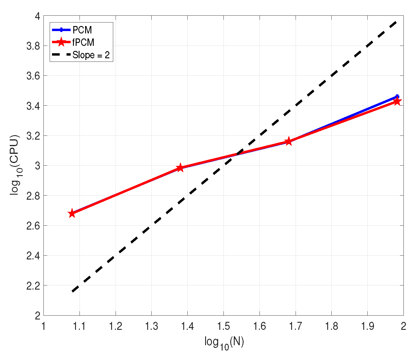
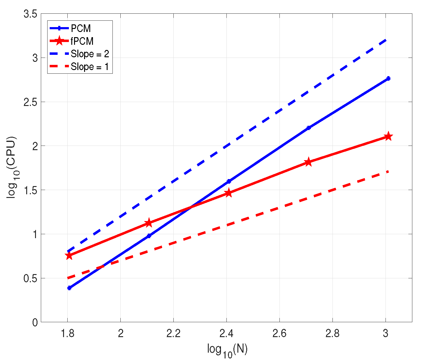
5. Numerical Examples

We present some numerical examples to check the convergence orders and the efficiency of the proposed predictor–corrector method (17) and fast predictor–corrector method (34). For convenience, we denote these two methods as PCM and fPCM, respectively.
Example 1.
Consider the following FDEs with α ( 0 , 1 ) :
C D 0 α y ( t ) = y ( t ) , t ( 0 , 1 ] ; y ( 0 ) = 1 .
The exact solution of (35) is y ( t ) = E α ( t α ) , where
E α ( s ) = k = 0 s k Γ ( α k + 1 )
is the Mittag-Leffler function.
Since
C D 0 α y ( t ) = 1 t α Γ ( α + 1 ) ( t α ) 2 Γ ( 2 α + 1 ) ,
that is, C D 0 α y ( t ) behaves as C ( 1 + t α ) . Set err N : = max 0 j N | y ( t j ) y j | and err N f : = max 0 j N | y ( t j ) y ¯ j | . Through Theorems 1 and 2, we have
err N C N min 2 r α , 3 and err N f C N min 2 r α , 3 + C ϵ ,
for PCM (17) and fPCM (34), respectively.
In our calculation, for fPCM, we take ϵ = 10 12 . In addition, to present the results, we define p : = log 2 E N / E 2 N to measure the convergence order of the methods, where E N can be err N or err N f . Applying PCM and fPCM to Problem (35) with different α and r, a series of numerical solutions can be obtained. For simplicity, in Table 1, we just display the maximal nodal errors, convergence orders, and CPU times in seconds of PCM and fPCM for Problem (35) with α = 0.5 . “EOC” in each column of p denotes the expected order of convergence presented in (36). “CPU" denotes the total CPU time in seconds for used methods to solve (35). As one may infer from Table 1, both PCM and fPCM almost had the same maximal nodal errors and convergence orders because, as shown in (36), the influence of the SOE approximation error ϵ could be negligible when it is chosen to be very small. In terms of CPU times, Figure 1 shows that fPCM took less time than PCM did, and this advantage is becoming more obvious with the increase in time steps N. When N was rather small compared to PCM, the fPCM was no longer efficient. Moreover, Figure 1 shows that the scales of PCM were like O ( N 2 ) , but the scales of fPCM were just like O ( N ) .
Example 2.
Consider the following Benjamin–Bona–Mahony–Burgers equation:
C D 0 α ( u u x x ) + u u x u x x = f ( x , t ) for ( x , t ) ( 0 , 1 ) × ( 0 , 1 ] ,
u ( x , 0 ) = sin ( π x ) for x [ 0 , 1 ] , u ( 0 , t ) = u ( 1 , t ) = 0 for t ( 0 , 1 ] ,
the function f, the initial-boundary value conditions are determined by exact solution u ( x , t ) = ( 1 + t α + t 2 α ) sin ( π x ) .
Similarly to (4), Equation (37) can be rewritten as the following integrodifferential equation.
u ( x , t ) u x x ( x , t ) = Q ( x ) + 1 Γ ( α ) s = 0 t ( t s ) α 1 F ( x , s , u ) d s for ( x , t ) ( 0 , 1 ) × ( 0 , 1 ] ,
where
Q ( x ) : = u ( x , 0 ) u x x ( x , 0 ) = ( 1 + π 2 ) sin ( π x ) ,
F ( x , t , u ) : = u x x ( x , t ) u ( x , t ) u x ( x , t ) + f ( x , t ) .
Let M be a positive integer. Set h = ( x R x L ) / M , x i = x L + i h for 0 i M . By applying the centered difference schemes δ x 2 v i = v i + 1 2 v i + v i 1 h 2 and Δ x v i = v i + 1 v i 1 2 h to numerically approximate u x x and u x , respectively, we can obtain the corresponding PCM and fPCM for (37).
One can check that
C D 0 α ( u u x x ) ( x , t ) = Γ ( α + 1 ) + 2 α Γ ( 2 α ) Γ ( 1 + α ) t α ( 1 + π 2 ) sin ( π x )
behaves as C ( 1 + t α ) . For 0 n N , 0 i M , set e i n = u ( x i , t n ) u i n , e ¯ i n = u ( x i , t n ) u ¯ i n , where u i n and u ¯ i n are the predictor–corrector method solution and the fast predictor–corrector method solution of (37). Set e n = e 1 n , e 2 n , , e M 1 n T and e ¯ n = e ¯ 1 n , e ¯ 2 n , , e ¯ M 1 n T . Similarly to [22], we use discrete H 1 norm to calculate the errors. Let E ( M , N ) : = max 0 j N e j H 1 and E ( M , N ) f : = max 0 j N e ¯ j H 1 . Then, one has
E ( M , N ) C ( N min 2 r α , 3 + h 2 ) and E ( M , N ) f C ( N min 2 r α , 3 + h 2 + ϵ )
for PCM and fPCM, respectively.
The numerical results are given in Table 2 and Table 3, where the convergence orders in time and space are calculated with
p t : = log 2 E M , N E M , 2 N , p x : = log 2 E M , N E 2 M , N ,
respectively, and E M , N can be E ( M , N ) or E ( M , N ) f . In the fPCM, we set ϵ = 10 8 . Table 2 and Table 3 show that PCM and fPCM almost had the same accuracy. In terms of CPU time, Table 3 and Figure 2 show that the fPCM offered no advantage when N was small, but when N was larger, the advantage of fPCM was obvious.

6. Concluding Remarks

A fast high-order predictor–corrector method was constructed for solving fractional differential equations. Graded meshes were used for time discretization to deal with the weak singularity of the solution near the initial time. Several numerical examples were presented to support our theoretical analysis. Since the predictor–corrector method failed to solve the stiff problem (see [6], Section 5), our fast high-order predictor–corrector method also had the same property. In future work, we will try to construct implicit–explicit methods by using the technique of our predictor–corrector method to solve the stiff fractional differential equations or time-fractional partial differential equations.

Author Contributions

Methodology, Y.Z.; writing—original draft preparation, X.S.; writing—review and editing, X.S. and Y.Z. All authors have read and agreed to the published version of the manuscript.

Funding

The work of Yongtao Zhou is supported in part by the China Postdoctoral Science Foundation under grant 2021M690322, and the National Natural Science Foundation of China for Young Scientists under grant 12101037.

Data Availability Statement

Not applicable.

Acknowledgments

The authors sincerely thank the reviewers for their constructive comments to improve the manuscript.

Conflicts of Interest

The authors declare no conflict of interest. The funders had no role in the design of the study; in the collection, analyses, or interpretation of data; in the writing of the manuscript; or in the decision to publish the results.

Abbreviations

The following abbreviations are used in this manuscript:
SOESum of exponentials
FDEsFractional differential equations
PCMPredictor–corrector method
fPCMFast predictor–corrector method

Appendix A. Proof of Lemma 4

Proof. 
By using | w ( t ) | C ( 1 + t α 1 ) , for t [ t 0 , t 1 ]
| w ( t ) Π 1 , 0 w ( t ) | = | t t 1 t 0 t 1 θ = t 0 t w ( θ ) d θ t t 0 t 1 t 0 θ = t t 1 w ( θ ) d θ | C θ = t 0 t 1 ( 1 + θ α 1 ) d θ C t 1 α ,
and, for t [ t 1 , t 2 ]
| w ( t ) Π 2 , 1 w ( t ) | = | w ( t ) t t 2 t 0 t 2 t t 1 t 0 t 1 w ( t 0 ) + t t 0 t 1 t 0 w ( t 1 ) t t 0 t 2 t 0 t t 2 t 1 t 2 w ( t 1 ) + t t 1 t 2 t 1 w ( t 2 ) | = | t t 2 t 0 t 2 w ( t ) t t 1 t 0 t 1 w ( t 0 ) t t 0 t 1 t 0 w ( t 1 ) t t 0 t 2 t 0 t t 2 t 1 t 2 w ( t 1 ) + t t 1 t 2 t 1 w ( t 2 ) w ( t ) | C | w ( t ) t t 1 t 0 t 1 w ( t 0 ) + t t 0 t 1 t 0 w ( t 1 ) | + C | w ( t ) t t 2 t 1 t 2 w ( t 1 ) + t t 1 t 2 t 1 w ( t 2 ) | = C | t t 1 t 0 t 1 θ = t 0 t w ( θ ) d θ t t 0 t 1 t 0 θ = t t 1 w ( θ ) d θ | + C | t t 2 t 1 t 2 θ = t 1 t w ( θ ) d θ t t 1 t 2 t 1 θ = t t 2 w ( θ ) d θ | C θ = t 0 t 2 ( 1 + θ α 1 ) d θ C t 2 α .
We similarly derive
| w ( t ) Π 1 , 0 w ( t ) | C t 2 α for t [ t 1 , t 2 ] , | w ( t ) Π 2 , 1 w ( t ) | C t 3 α for t [ t 2 , t 3 ] .
We first consider the estimate of I 1 n + 1 . When n = 0 , with the use of (7) and (A1), we obtain
I 1 1 = | s = t 0 t 1 ( t 1 s ) α 1 ( w Π 1 , 0 w ) ( s ) d s | C s = t 0 t 1 ( t 1 s ) α 1 t 1 α d s C t 1 2 α C N 2 r α .
When n = 1 , it follows from (7), (A1), and (A2) that
I 1 2 = | s = t 0 t 1 ( t 2 s ) α 1 ( w Π 1 , 0 w ) ( s ) d s + s = t 1 t 2 ( t 2 s ) α 1 ( w Π 2 , 1 w ) ( s ) d s | C s = t 0 t 1 ( t 2 s ) α 1 t 1 α d s + C s = t 1 t 2 ( t 2 s ) α 1 t 2 α d s C t 2 α s = t 0 t 2 ( t 2 s ) α 1 d s C t 2 2 α C N 2 r α .
For some ξ ( t j 1 , t j + 1 )
w ( t ) Π 2 , j w ( t ) = w ( ξ ) 6 ( t t j 1 ) ( t t j ) ( t t j + 1 ) for t [ t j 1 , t j + 1 ] .
Then, when n 2 , one obtains from | w ( t ) | C ( 1 + t α 3 ) , (A1), (A2) and (A4) that
I 1 n + 1 | s = t 0 t 1 ( t n + 1 s ) α 1 ( w Π 1 , 0 w ) ( s ) d s + s = t 1 t 2 ( t n + 1 s ) α 1 ( w Π 2 , 1 w ) ( s ) d s | + | j = 2 n 2 s = t j t j + 1 ( t n + 1 s ) α 1 ( w Π 2 , j w ) ( s ) d s | + | j = n 2 + 1 n 1 s = t j t j + 1 ( t n + 1 s ) α 1 ( w Π 2 , j w ) ( s ) d s | + | s = t n t n + 1 ( t n + 1 s ) α 1 ( w Π 2 , n w ) ( s ) d s | C | s = t 0 t 2 ( t n + 1 s ) α 1 t 2 α d s | + C | j = 2 n 2 t j 1 α 3 τ j + 1 3 s = t j t j + 1 ( t n + 1 s ) α 1 d s | + C | j = n 2 + 1 n 1 t j 1 α 3 τ j + 1 3 s = t j t j + 1 ( t n + 1 s ) α 1 d s | + C | t n 1 α 3 τ n + 1 3 s = t n t n + 1 ( t n + 1 s ) α 1 d s | : = I 1 , 1 n + 1 + I 1 , 2 n + 1 + I 1 , 3 n + 1 + I 1 , 4 n + 1 .
For I 1 , 1 n + 1 , we can obtain from (7) that
I 1 , 1 n + 1 C ( t n + 1 t 2 ) α 1 t 2 α + 1 C N 2 r α ( n + 1 ) r 2 r α 1 C N 2 r α .
For I 1 , 2 n + 1 , recalling (7) and noting that, for 2 j n 2
( t n + 1 t j + 1 ) α 1 C N r ( n + 1 ) r ( j + 1 ) r 1 α C N r ( n + 1 ) r ( n 2 + 1 ) r 1 α C ( N / n ) r ( 1 α ) .
Therefore
I 1 , 2 n + 1 C j = 2 n 2 t j 1 α 3 τ j + 1 4 ( t n + 1 t j + 1 ) α 1 C N 2 r α j = 2 n 2 j 2 r α 4 ( j / n ) r ( 1 α ) C N 2 r α j = 2 n 2 j 2 r α 4 C N 2 r α for 1 r < 3 2 α , N 3 ln N for r = 3 2 α , N 3 for r > 3 2 α ,
where the well-known convergence results for series
j = 1 n j β 1 C 1 for β < 0 , ln n for β = 0 , n γ for β > 0 ,
was used. For I 1 , 3 n + 1 , with the use of (7), one obtains for n 2 + 1 j n 1 that
t j 1 α 3 C [ ( j 1 ) / N ] r ( α 3 ) C n 2 / N r ( α 3 ) C ( n / N ) r ( α 3 ) .
Then, one sees that
I 1 , 3 n + 1 C N r α n r α 3 s = t n 2 + 1 t n ( t n + 1 s ) α 1 d s C N r α n r α 3 ( t n + 1 t n 2 + 1 ) α ( t n + 1 t n ) α C N r α n r α 3 ( t n + 1 ) α C N 2 r α n 2 r α 3 C N 2 r α for 1 r < 3 2 α , N 3 for r 3 2 α .
For I 1 , 4 n + 1 , again by using (7), one can obtain that
I 1 , 4 n + 1 C t n 1 α 3 τ n + 1 3 + α C N 2 r α n 2 r α 3 α C N 2 r α for 1 r < 3 + α 2 α , N 3 α for r 3 + α 2 α .
Substituting (A6)–(A9) into (A5) gives
I 1 n + 1 C N 2 r α for 1 r < 3 2 α , N 3 ln N for r = 3 2 α , N 3 for r > 3 2 α , with 0 n N 1 .
Next, to estimate I 2 n + 1 , when n = 0 , it follows from | w ( t ) | C ( 1 + t α 1 ) and (7) that
I 2 1 = s = t 0 t 1 ( t 1 s ) α 1 ( w ( s ) w ( t 0 ) ) d s C s = t 0 t 1 ( t 1 s ) α 1 θ = t 0 s w ( θ ) d θ d s C s = t 0 t 1 ( t 1 s ) α 1 θ = t 0 s ( 1 + θ α 1 ) d θ d s C s = t 0 t 1 ( t 1 s ) α 1 s α d s C t 1 2 α C N 2 r α .
When n = 1 , by using (7), (A1), and (A3),
I 2 2 = | s = t 0 t 2 ( t 2 s ) α 1 ( w Π 1 , 0 w ) ( s ) d s | C s = t 0 t 2 ( t 2 s ) α 1 t 2 α d s C t 2 2 α C N 2 r α .
When n = 2 , from (7), (A1), (A2) and (A3), one obtains
I 2 3 = | s = t 0 t 1 ( t 3 s ) α 1 ( w Π 1 , 0 w ) ( s ) d s + s = t 1 t 3 ( t 3 s ) α 1 ( w Π 2 , 1 w ) ( s ) d s | C s = t 0 t 1 ( t 3 s ) α 1 t 1 α d s + C s = t 1 t 3 ( t 3 s ) α 1 t 3 α d s C ( t 3 t 1 ) α 1 t 1 α + 1 + C ( t 3 t 1 ) α t 3 α C N 2 r α .
When n 3 ,
I 2 n + 1 | s = t 0 t 1 ( t n + 1 s ) α 1 ( w Π 1 , 0 w ) ( s ) d s + s = t 1 t 2 ( t n + 1 s ) α 1 ( w Π 2 , 1 w ) ( s ) d s | + | j = 2 n 2 s = t j t j + 1 ( t n + 1 s ) α 1 ( w Π 2 , j w ) ( s ) d s | + | j = n 2 + 1 n 1 s = t j t j + 1 ( t n + 1 s ) α 1 ( w Π 2 , j w ) ( s ) d s | + | s = t n t n + 1 ( t n + 1 s ) α 1 ( w Π 2 , n 1 w ) ( s ) d s | C | s = t 0 t 2 ( t n + 1 s ) α 1 t 2 α d s | + C | j = 2 n 2 t j 1 α 3 τ j + 1 3 s = t j t j + 1 ( t n + 1 s ) α 1 d s | + C | j = n 2 + 1 n 1 t j 1 α 3 τ j + 1 3 s = t j t j + 1 ( t n + 1 s ) α 1 d s | + C | t n 2 α 3 τ n + 1 3 s = t n t n + 1 ( t n + 1 s ) α 1 d s | : = I 1 , 1 n + 1 + I 1 , 2 n + 1 + I 1 , 3 n + 1 + I 2 , 1 n + 1 ,
the difference to I 1 n + 1 is just the last term I 2 , 1 n + 1 . One obtains from (7) that
I 2 , 1 n + 1 C t n 2 α 3 τ n + 1 3 + α C N 2 r α n 2 r α 3 α C N 2 r α for 1 r < 3 + α 2 α , N 3 α for r 3 + α 2 α .
Hence, we have
I 2 n + 1 C N 2 r α for 1 r < 3 2 α , N 3 ln N for r = 3 2 α , N 3 for r > 3 2 α , with 0 n N 1 .
Therefore, synthesizing the above results, the lemma is proved. □

References

  1. Diethelm, K. The Analysis of Fractional Differential Equations; Lecture Notes in Mathematics; Springer: Berlin, Germany, 2010; Volume 2004, pp. viii+247. [Google Scholar]
  2. Jin, B.; Lazarov, R.; Zhou, Z. Numerical methods for time-fractional evolution equations with nonsmooth data: A concise overview. Comput. Methods Appl. Mech. Engrg. 2019, 346, 332–358. [Google Scholar] [CrossRef]
  3. Chen, H.; Stynes, M. Error analysis of a second-order method on fitted meshes for a time-fractional diffusion problem. J. Sci. Comput. 2019, 79, 624–647. [Google Scholar] [CrossRef]
  4. Kopteva, N.; Meng, X. Error analysis for a fractional-derivative parabolic problem on quasi-graded meshes using barrier functions. SIAM J. Numer. Anal. 2020, 58, 1217–1238. [Google Scholar] [CrossRef]
  5. Stynes, M.; O’Riordan, E.; Gracia, J.L. Error analysis of a finite difference method on graded meshes for a time-fractional diffusion equation. SIAM J. Numer. Anal. 2017, 55, 1057–1079. [Google Scholar] [CrossRef]
  6. Cao, W.; Zeng, F.; Zhang, Z.; Karniadakis, G.E. Implicit-explicit difference schemes for nonlinear fractional differential equations with nonsmooth solutions. SIAM J. Sci. Comput. 2016, 38, A3070–A3093. [Google Scholar] [CrossRef]
  7. Diethelm, K.; Freed, A.D. The FracPECE subroutine for the numerical solution of differential equations of fractional order. Forsch. Und Wiss. Rechn. 1998, 1999, 57–71. [Google Scholar]
  8. Diethelm, K.; Ford, N.J. Analysis of fractional differential equations. J. Math. Anal. Appl. 2002, 265, 229–248. [Google Scholar] [CrossRef]
  9. Diethelm, K.; Ford, N.J.; Freed, A.D. A predictor-corrector approach for the numerical solution of fractional differential equations. Nonlinear Dyn. 2002, 29, 3–22. [Google Scholar] [CrossRef]
  10. Diethelm, K.; Ford, N.J.; Freed, A.D. Detailed error analysis for a fractional Adams method. Numer. Algorithms 2004, 36, 31–52. [Google Scholar] [CrossRef]
  11. Li, C.; Yi, Q.; Chen, A. Finite difference methods with non-uniform meshes for nonlinear fractional differential equations. J. Comput. Phys. 2016, 316, 614–631. [Google Scholar] [CrossRef]
  12. Liu, Y.; Roberts, J.; Yan, Y. Detailed error analysis for a fractional Adams method with graded meshes. Numer. Algorithms 2018, 78, 1195–1216. [Google Scholar] [CrossRef] [Green Version]
  13. Liu, Y.; Roberts, J.; Yan, Y. A note on finite difference methods for nonlinear fractional differential equations with non-uniform meshes. Int. J. Comput. Math. 2018, 95, 1151–1169. [Google Scholar] [CrossRef]
  14. Lubich, C. Fractional linear multistep methods for Abel-Volterra integral equations of the second kind. Math. Comp. 1985, 45, 463–469. [Google Scholar] [CrossRef]
  15. Zhou, Y.; Suzuki, J.L.; Zhang, C.; Zayernouri, M. Implicit-explicit time integration of nonlinear fractional differential equations. Appl. Numer. Math. 2020, 156, 555–583. [Google Scholar] [CrossRef]
  16. Inc, M. The approximate and exact solutions of the space-and time-fractional Burgers equations with initial conditions by variational iteration method. J. Math. Anal. Appl. 2008, 345, 476–484. [Google Scholar] [CrossRef]
  17. Jafari, H.; Daftardar-Gejji, V. Solving linear and nonlinear fractional diffusion and wave equations by Adomian decomposition. Appl. Math. Comput. 2006, 180, 488–497. [Google Scholar] [CrossRef]
  18. Jin, B.; Lazarov, R.; Pasciak, J.; Zhou, Z. Error analysis of a finite element method for the space-fractional parabolic equation. SIAM J. Numer. Anal. 2014, 52, 2272–2294. [Google Scholar] [CrossRef]
  19. Zayernouri, M.; Karniadakis, G.E. Discontinuous spectral element methods for time- and space-fractional advection equations. SIAM J. Sci. Comput. 2014, 36, B684–B707. [Google Scholar] [CrossRef]
  20. Deng, W. Short memory principle and a predictor-corrector approach for fractional differential equations. J. Comput. Appl. Math. 2007, 206, 174–188. [Google Scholar] [CrossRef]
  21. Nguyen, T.B.; Jang, B. A high-order predictor-corrector method for solving nonlinear differential equations of fractional order. Fract. Calc. Appl. Anal. 2017, 20, 447–476. [Google Scholar] [CrossRef]
  22. Zhou, Y.; Li, C.; Stynes, M. A fast second-order predictor-corrector method for a nonlinear time-fractional Benjamin-Bona-Mahony-Burgers equation. 2022; submitted to Numer. Algorithms. [Google Scholar]
  23. Zhou, Y.; Stynes, M. Block boundary value methods for linear weakly singular Volterra integro-differential equations. BIT Numer. Math. 2021, 61, 691–720. [Google Scholar] [CrossRef]
  24. Zhou, Y.; Stynes, M. Block boundary value methods for solving linear neutral Volterra integro-differential equations with weakly singular kernels. J. Comput. Appl. Math. 2022, 401, 113747. [Google Scholar] [CrossRef]
  25. Zhou, B.; Chen, X.; Li, D. Nonuniform Alikhanov linearized Galerkin finite element methods for nonlinear time-fractional parabolic equations. J. Sci. Comput. 2020, 85, 39. [Google Scholar] [CrossRef]
  26. Lubich, C. Discretized fractional calculus. SIAM J. Math. Anal. 1986, 17, 704–719. [Google Scholar] [CrossRef]
  27. Zeng, F.; Zhang, Z.; Karniadakis, G.E. Second-order numerical methods for multi-term fractional differential equations: Smooth and non-smooth solutions. Comput. Methods Appl. Mech. Engrg. 2017, 327, 478–502. [Google Scholar] [CrossRef]
  28. Li, D.; Sun, W.; Wu, C. A novel numerical approach to time-fractional parabolic equations with nonsmooth solutions. Numer. Math. Theory Methods Appl. 2021, 14, 355–376. [Google Scholar]
  29. She, M.; Li, D.; Sun, H.w. A transformed L1 method for solving the multi-term time-fractional diffusion problem. Math. Comput. Simul. 2022, 193, 584–606. [Google Scholar] [CrossRef]
  30. Lubich, C. Runge-Kutta theory for Volterra and Abel integral equations of the second kind. Math. Comp. 1983, 41, 87–102. [Google Scholar] [CrossRef]
  31. Jiang, S.; Zhang, J.; Zhang, Q.; Zhang, Z. Fast evaluation of the Caputo fractional derivative and its applications to fractional diffusion equations. Commun. Comput. Phys. 2017, 21, 650–678. [Google Scholar] [CrossRef]
  32. Li, D.; Zhang, C. Long time numerical behaviors of fractional pantograph equations. Math. Comput. Simul. 2020, 172, 244–257. [Google Scholar] [CrossRef]
  33. Yan, Y.; Sun, Z.Z.; Zhang, J. Fast evaluation of the Caputo fractional derivative and its applications to fractional diffusion equations: A second-order scheme. Commun. Comput. Phys. 2017, 22, 1028–1048. [Google Scholar] [CrossRef]
  34. Liao, H.l.; Tang, T.; Zhou, T. A second-order and nonuniform time-stepping maximum-principle preserving scheme for time-fractional Allen-Cahn equations. J. Comput. Phys. 2020, 414, 109473. [Google Scholar] [CrossRef] [Green Version]
  35. Ran, M.; Lei, X. A fast difference scheme for the variable coefficient time-fractional diffusion wave equations. Appl. Numer. Math. 2021, 167, 31–44. [Google Scholar] [CrossRef]
Figure 1. Total number of time steps N versus CPU times of PCM and fPCM in log–log scale for Problem (35) with r = 3 / ( 2 α ) .
Fractalfract 06 00516 g001
Figure 2. Total number of time steps N versus CPU times of PCM and fPCM in log–log scale for Problem (37) with α = 0.8 and r = 3 / ( 2 α ) .
Fractalfract 06 00516 g002
Table 1. Maximal nodal errors, convergence orders, and CPU times of PCM and fPCM for Problem (35) with α = 0.5 .
PCM fPCM
Nr err N pCPU err N f pCPU
641 1.1732 × 10 3 2.58 1.1732 × 10 3 3.34
128 6.9056 × 10 4 0.76469.51 6.9056 × 10 4 0.76466.95
256 4.1422 × 10 4 0.737439.85 4.1422 × 10 4 0.737414.99
512 2.3219 × 10 4 0.8351162.84 2.3219 × 10 4 0.835132.26
1024 1.2514 × 10 4 0.8917638.56 1.2514 × 10 4 0.891767.66
EOC 1 1
64 r = 2 2 α 1.0150 × 10 4 2.41 1.0150 × 10 4 4.68
128 1.8584 × 10 5 2.44939.61 1.8584 × 10 5 2.44939.97
256 4.2737 × 10 6 2.120539.23 4.2737 × 10 6 2.120522.57
512 1.0898 × 10 6 1.9715157.12 1.0898 × 10 6 1.971548.61
1024 2.7510 × 10 7 1.9860639.94 2.7510 × 10 7 1.9860107.74
EOC 2 2
64 r = 3 2 α 8.3324 × 10 6 2.44 8.3324 × 10 6 5.71
128 8.1803 × 10 7 3.34859.53 8.1803 × 10 7 3.348513.35
256 9.6599 × 10 8 3.082139.48 9.6599 × 10 8 3.082129.22
512 1.2096 × 10 8 2.9975159.67 1.2096 × 10 8 2.997565.48
1024 1.5129 × 10 9 2.9991580.18 1.5129 × 10 9 2.9991128.07
EOC 3 3
64 r = 4 2 α 3.5974 × 10 6 2.41 3.5974 × 10 6 6.95
128 3.6817 × 10 7 3.28858.71 3.6817 × 10 7 3.288515.04
256 4.1714 × 10 8 3.141835.14 4.1714 × 10 8 3.141833.36
512 4.9751 × 10 9 3.0677142.50 4.9751 × 10 9 3.067773.69
1024 6.0885 × 10 10 3.0306568.88 6.0883 × 10 10 3.0306159.33
EOC 3 3
Table 2. Maximal nodal errors and convergence orders of PCM and fPCM for Problem (37) with r = 3 / ( 2 α ) and M = 8000 .
α = 0.4 α = 0.6 α = 0.8
Scheme N E M , N p t E M , N p t E M , N p t
PCM12 6.4472 × 10 2 3.8631 × 10 3 4.8683 × 10 4
24 3.1108 × 10 3 4.3733 2.5987 × 10 4 3.8939 4.4781 × 10 5 3.4425
48 1.7218 × 10 4 4.1753 2.2876 × 10 5 3.5058 5.7787 × 10 6 2.9541
96 1.1986 × 10 5 3.8445 2.4634 × 10 6 3.2151 7.9723 × 10 7 2.8577
EOC 3 3 3
fPCM12 6.4472 × 10 2 3.8631 × 10 3 4.8683 × 10 4
24 3.1108 × 10 3 4.3733 2.5987 × 10 4 3.8939 4.4781 × 10 5 3.4425
48 1.7218 × 10 4 4.1753 2.2876 × 10 5 3.5058 5.7787 × 10 6 2.9541
96 1.1986 × 10 5 3.8445 2.4634 × 10 6 3.2151 7.9723 × 10 7 2.8577
EOC 3 3 3
Table 3. Maximal nodal errors, convergence orders, and CPU times of PCM and fPCM for Problem (37) with α = 0.8 , r = 3 / ( 2 α ) and N = 2000 .
PCM fPCM
M E ( M , N ) p x CPU E ( M , N ) f p x CPU
8 8.9024 × 10 2 1.93772141.30 8.9024 × 10 2 1.9377134.57
16 2.2690 × 10 2 1.97222131.37 2.2690 × 10 2 1.9722133.85
32 5.7260 × 10 3 1.98642164.59 5.7260 × 10 3 1.9864132.92
64 1.4382 × 10 3 1.99322158.93 1.4382 × 10 3 1.9933137.41
EOC 2 2
Publisher’s Note: MDPI stays neutral with regard to jurisdictional claims in published maps and institutional affiliations.

