Fractional Model of the Deformation Process

Abstract

The article considers the fractional Poisson process as a mathematical model of deformation activity in a seismically active region. The dislocation approach is used to describe five modes of the deformation process. The change in modes is determined by the change in the intensity of the event stream, the regrouping of dislocations, and the change in and the appearance of stable connections between dislocations. Modeling of the change of deformation modes is carried out by changing three parameters of the proposed model. The background mode with independent events is described by a standard Poisson process. To describe variations from the background mode of seismic activity, when connections are formed between dislocations, the fractional Poisson process and the Mittag–Leffler function characterizing it are used. An approximation of the empirical cumulative distribution function of waiting time of the foreshocks obtained as a result of processing the seismic catalog data was carried out on the basis of the proposed model. It is shown that the model curves, with an appropriate choice of the Mittag–Leffler function’s parameters, gives results close to the experimental ones and can be allowed to characterize the deformation process in the seismically active region under consideration.

1. Introduction

A large number of studies have been devoted to study the correlations between seismic events [1,2,3,4]. The laws of Gutenberg–Richter and Omori–Utsu, the property of clustering in aftershock and foreshock sequences, and swarms of earthquakes, among other things, are well known. [5,6,7]. A block-hierarchical approach [4], an ETAS model [3,8], methods for identifying the main energy branches [9,10,11,12,13], and methods for studying complex networks [14] have been used to study the correlations and to determine the criteria of seismic event connectivity, which are considered as a stream of random events in some volume. The theory of fractals and fractional processes is widely applied in studies of the seismic process and in the construction of its models. The medium characteristics, the structure of fault networks [15], and the set of the epicenters of earthquakes [16] have a fractal nature and are determined by fractional laws [3,14,17]. The result of a large number of constructed statistical models was the conclusion that there is a correlation between seismic events in the catalogs under consideration based on the selected criteria [3,6,7,10,11,12,17,18,19,20]. In this case, the seismic process representation as a stream of independent events and its description by standard Poisson process becomes incorrect [2,19,21]. Correlations between events in these sequences leads to the appearance of the properties of hereditarity (non-locality in time, «memory») and non-locality in space. The use of the fractional Poisson process to describe the process of seismic deformations is a logical continuation of this approach, which takes into account properties of non-locality [22].

This article is a continuation of the works [12,13,22]. The fractional Poisson process is used to describe irreversible deformation changes [22]. The proposed model of the seismic deformation process includes five modes, each of which is determined by a change in the values of the fractional Poisson process parameters. To verify of the fractional model of the deformation process, foreshock sequences constructed on the base of a seismic catalog data [23] by a statistical model are used [12]. This phase of seismic deformational process activation is of interest from the point of view of seismic hazard assessment. The deformations can be considered a sequence of independent random dislocation changes. The standard Poisson process can serve as a model of such changes. To account for non-locality effects, the authors propose the use of a fractional Poisson process [22]. The transition in this investigation to a multiparametric fractional Poisson process expands the possibilities of describing deformation changes. It is possible to consider not only exponential, but also power-law correlations between seismic events, which makes it possible to model both normal and abnormal activation and relaxation processes. The analytical dependencies compare with the results of catalog data processing obtained on the base on the criteria of event connectivity.

2. Mathematical Model of the Deformation Process

As noted in reference [22], the critical level of elastic stresses is sustained by the work of external forces. The result of their actions is a deformation process with a change of the deformation modes. This process is characterized by the rate of random changes of dislocations, which are determined by the spatial scale and the value of the displacement vector. This approach describes discontinuities, movements along existing faults, and repackaging of grains or blocks in a wide range of scales using the theory of dislocation changes.

Each dislocation is defined by spatial-temporal coordinates. The distribution of the set of dislocation changes in the considered volume over the time is a random process. If the areas of influence of the dislocations does not intersect, then they are considered independent. In this case, the process of dislocation repackaging is defined as a random walk process and is described by a standard Poisson process. If the density of dislocations increases and their areas of influence overlap, then the dislocations become correlated and a dislocation cluster is formed. Then, in the spatial-temporal representation, the cluster is described by a fractional Poisson process. We apply this generalization of the standard Poisson process as a model for describing irreversible changes in deformation process. The fractional Poisson process makes it possible to obtain a variety of activation and relaxation processes of three types: $e^{\pm t}$, $e^{\pm t^{\alpha }}$, and $t^{\pm \alpha }$. The last type of power law dependence arises due to hereditarity effects, corresponds to fractal properties and gives the abnormal activation and relaxation of the process.

The processes of dislocation change has the same structure at different scale levels of the deformation process. Therefore, to describe the model, it is sufficient to consider the deformation process for one selected spatial scale.

The deformation activity is decomposed into five modes or states: $s_1$—the background mode (background or normal pulsations); $s_2$—the decaying mode (deceleration pulsations); $s_3$—the activation mode in the phase of foreshocks; $s_4$—the activation mode in the phase of the main shock; and $s_5$—the relaxation mode in the phase of aftershocks. We describe each state and the probability of its preservation in the same state or transition to another one using the concept of a fractional Poisson process and the Mittag–Leffler function with a power law argument, which defines the relaxation or activation (depending on the sign change) characteristic of the deformation process,

$$E_{\nu }(-{\left(\mu t\right)}^{\tilde{\nu }})=\sum _{k=0}^{\infty }\frac{{(-{\left(\mu t\right)}^{\tilde{\nu }})}^k}{\Gamma (1+\nu k)},$$

(1)

where the parameter $\nu$ ($0<\nu \le 1$) is the fractional parameter of the Poisson process (the parameter of the fractional derivative), and the parameter $\tilde{\nu }$ is a non-stationarity parameter, i.e., a power law dependence on the time of the non-stationary event stream if the parameter value satisfies the condition $0<\tilde{\nu }<1$. The function $E_{\nu }\left(x\right)$ gives a description of the hereditarity effects (when $\nu$ decreases, hereditarity of the process increases), and the power law argument ${\left(\mu t\right)}^{\tilde{\nu }}$ determines the power law change of the dislocation stream intensity. Function $x=e^{-{\left(\mu t\right)}^{\tilde{\nu }}}$ is the power law exponential one, which obeys a differential equation,

$${\displaystyle \frac{dx}{dt}}=-x\mu \tilde{\nu }{\left(\mu t\right)}^{\tilde{\nu }-1}$$

for a process x in which the intensity of the dislocation stream varies locally with time according to a power law. Together, ${\left(\mu t\right)}^{\tilde{\nu }}$ and $E_{\nu }\left(x\right)$ define the complicated delayed relaxation (gives a non-local effect) (Figure 1(II)).

Thus, by varying the parameters $\nu$ and $\tilde{\nu }$, it is possible to obtain different modes of the deformation process with the predominance of the hereditarity properties («memory» or non-locality) or locality (power law exponential function of local branching processes), respectively. The temporal and spatial properties of wave processes with non-exponential correlations between events are related by dispersion relations (for example, the pulse duration of acoustic emission is related to the crack size, and the waiting time between pulses is related to the distances between cracks); therefore, if the process has temporal nonlocality, then it also has spatial non-locality. When the activation phase of the process begins, memory effects occur, and with them, the effects of spatial nonlocality of the seismic events branching occur.

State$s_1$. Within the framework of this approach, the background process of seismic deformations is a standard Poisson process (a stream of independent events) with an average intensity $\mu$. Then the probability of remaining in the same state exponentially depends on the time (Figure 1(I)) and is defined as

$$P_{11}\left(t\right)=e^{-\mu t}=E_1(-\mu t),$$

(2)

and the transition probability of the process to the next state is given as follows: $P_{12}\left(t\right)=1-e^{-\mu t}=1-E_1(-\mu t)$.

State$s_2$. Variation from the background mode occurs as a result of constantly acting external forces and leads to a change in rheology. If, in some volume V of space, a local hardening of the medium occurs at the instant of time $t^{\prime }$, then the deformation process slows down, and the intensity $\mu$ of the stream of events decreases and becomes equal to $\widehat{\mu }$ (an area of seismic gap [24], in which a deformation inhomogeneity is formed). Thus, there is an energy accumulation of adjourned (unfulfilled) events, which are localized in a volume V and are formed into a cluster. As a consequence of this, the waiting time interval increases for each following occurring event, which indicates the heredity of the process. Then, the probability of the remaining the process in the state $s_2$ can be given by the decreasing fractional Mittag–Leffler function (1) with the following parameters: $\widehat{\mu }t>{(\Gamma (1+\nu ))}^{-\frac{1}{1+\tilde{\nu }}}$, $0<\nu \le 1$, and $0<\tilde{\nu }\le 1$ [25,26]

$$P_{22}\left(t\right)=E_{\nu }(-{\left(\widehat{\mu }t\right)}^{\tilde{\nu }})=\sum _{k=0}^{\infty }{\displaystyle \frac{{(-{\left(\widehat{\mu }t\right)}^{\tilde{\nu }})}^k}{\Gamma (1+\nu k)}}.$$

(3)

The probability $P_{22}\left(t\right)$ (3) at the initial stage decreases faster than the exponential function (2), and as the time interval increases, it decreases more slowly (Figure 1(II)), i.e., the process is delayed in time. This indicates the presence of aftereffects or hereditarity effects in the fractional process due to the clustering of events that did not occurr in the seismic gap.

We should note that the parameter $\nu$ is defined the fractional dimension of the event distribution over the time interval [26]. Thus, the medium hardening changes the fractional order of the process (statistics of events), which detects a delayed relaxation caused by the effects of hereditarity that arose as a result of hardening.

State$s_3$. The event shortages in the state $s_2$ leads to an increase in elastic stresses, as a result of which the medium hardening is overcome and the intensity $\widehat{\mu }$ of the event stream increases and takes the value $\tilde{\mu }$, and the accumulated additional elastic energy is released. The result of that is a deformation perturbation that occurs at the instant of time $t^{\prime }$ and a transition to the state $s_3$, the phase of foreshocks, which ends with the mainshock (transition to the state $s_4$). This activation can be considered as an event of a higher scale in relation to events that were unfulfilled in the seismic gap, and the energy of the deformation disturbance should correspond to the sum of the energies of the unfulfilled events.

For an analytical description of the state $s_3$, we use the probability of the mainshock occurrence at the instant of time $t^{*}$ ($t<t^{*}$), i.e., the probability $P_{34}\left(t\right)$ of transition from state $s_3$ to state $s_4$. We give the probability $P_{34}\left(t\right)$ by the increasing Mittag–Leffler fractional function (1) as follows (Figure 2):

$$P_{34}\left(t\right)=E_{\nu }(-{\left[\tilde{\mu }(t^{*}-t)\right]}^{\tilde{\nu }})=\sum _{k=0}^{\infty }\frac{{(-{\left[\tilde{\mu }(t^{*}-t)\right]}^{\tilde{\nu }})}^k}{\Gamma (1+\nu k)},$$

(4)

where $\tilde{\mu }$—is the average intensity of the event stream in the deformation perturbation, $0<\nu \le 1$, $0<\tilde{\nu }\le 1$. In this case, the probability of not changing the state $s_3$ is given by the expression $P_{33}\left(t\right)=1-P_{34}\left(t\right)=1-E_{\nu }(-{\left[\tilde{\mu }(t^{*}-t)\right]}^{\tilde{\nu }})$.

Differentiating the expression (4), we obtain the probability density of distribution of the increasing stream of foreshocks, which can be interpreted as the inverse Omori–Utsu’s law,

$$\frac{d{P}_{34}\left(t\right)}{dt}=\frac{d{E}_{\nu }(-{\left[\tilde{\mu }(t^{*}-t)\right]}^{\tilde{\nu }})}{dt}=\sum _{k=0}^{\infty }\frac{{(-1)}^{k+1}\tilde{\mu }\tilde{\nu }k{\left(\tilde{\mu }(t^{*}-t)\right)}^{\tilde{\nu }k-1}}{\Gamma (1+\nu k)}.$$

The phase of foreshocks as well as the damping phase preceding it are interesting for the purpose of earthquake prediction. The energy of stress discharge can be evaluated from the decay time, and the development rate of a deformation disturbance can be predicted from the period of foreshocks, which gives the time of a short-term forecast.

State$s_4$. When the function $P_{34}\left(t\right)$ reaches a value equal to one, the process goes to the state $s_4$ of the mainshock with the maximum density of dislocations. The probability $P_{44}\left(t\right)$ of remaining in the state $s_4$ of the mainshock that occurred at instant of time $t^{*}$, for the values $t>t^{*}$, is given by the decreasing Mittag–Leffler fractional function (1):

$$P_{44}\left(t\right)=1-E_{{\nu }^{\prime }}(-{\left[\tilde{\mu }(t-t^{*})\right]}^{{\tilde{\nu }}^{\prime }})=1-\sum _{k=0}^{\infty }\frac{{(-{\left[\tilde{\mu }(t-t^{*})\right]}^{{\tilde{\nu }}^{\prime }})}^k}{\Gamma (1+{\nu }^{\prime }k)},$$

where $0<{\nu }^{\prime }\le 1$, $0<{\tilde{\nu }}^{\prime }\le 1$.

State$s_5$. As a result of the mainshock, the medium weakens (rheology changes), which leads to a gradual decrease in the density of dislocations and the event stream intensity $\tilde{\mu }$, which takes the value ${\tilde{\mu }}^{\prime }$. The process is inverse to the phase of foreshocks; consequently, the phase of aftershocks can be defined similarly to the state $s_3$. The probability $P_{45}\left(t\right)$ of transition to state $s_5$, the aftershock phase, is defined as the probability of the non-preservation mainshock (Figure 3).

$$P_{45}\left(t\right)=1-P_{44}\left(t\right)=E_{{\nu }^{\prime }}(-{\left[{\tilde{\mu }}^{\prime }(t-t^{*})\right]}^{{\tilde{\nu }}^{\prime }})=\sum _{k=0}^{\infty }\frac{{(-{\left[{\tilde{\mu }}^{\prime }(t-t^{*})\right]}^{{\tilde{\nu }}^{\prime }})}^k}{\Gamma (1+{\nu }^{\prime }k)}.$$

(5)

Differentiating expression (5), we obtain the density of decreasing the stream of aftershocks, i.e., Omori–Utsu’s law,

$$\frac{d{P}_{45}\left(t\right)}{dt}=\frac{d{E}_{{\nu }^{\prime }}(-{[{\tilde{\mu }}^{\prime }(t-t^{*})]}^{{\tilde{\nu }}^{\prime }})}{dt}=\sum _{k=0}^{\infty }\frac{{(-1)}^k{\tilde{\mu }}^{\prime }{\tilde{\nu }}^{\prime }k{\left({\tilde{\mu }}^{\prime }(t-t^{*})\right)}^{{\tilde{\nu }}^{\prime }k-1}}{\Gamma (1+{\nu }^{\prime }k)}.$$

3. Statistical Model of the Foreshock Mode

3.1. Algorithm for Constructing Sequences of Foreshocks

We use the criteria defined in works [12,13] to construct a statistical model. Two events are correlated if they satisfy the spatial criterion, which is determined by the medium inhomogeneity [27], the temporal criterion derived from Gutenberg–Richter’s law, and the energy criterion, according to which the events preceding the mainshock have less energy (magnitude or energy class). The construction of a sequence of correlated seismic events forming a cluster is determined by the proximity of preceding events to the initiated one based on the introduced criteria.

The identification of preceding events as a foreshock is carried out according to the following algorithm. The spatial-temporal area of the mainshock preparation is determined by the spatial $R_d$ and temporal $R_t$ scales, depending on the energy class of the event being prepared [12,13]. The preceding earthquake is considered a foreshock and is included in the sequence (cluster) if the following conditions are satisfied:

(1)

The time interval between the mainshock and the preceding event does not exceed the time scale $R_t$: $\Delta t=(t_j-t_i)\le R_t$;

(2)

The distance between the mainshock and the preceding event does not exceed the spatial scale $R_d$: $\Delta d=|{\mathbf{r}}_j-{\mathbf{r}}_i|\le R_d$, where r is the radius-vector before the event;

(3)

The energy class of the preceding event is less than the class K of the mainshock.

If an event is marked as a foreshock, then the same algorithm is applied to it, i.e., we make the transition to a lower energy level and find foreshocks for this event, etc. Thus, we proceed down the levels.

The algorithm works if the events (foreshocks) of lower energy get into the spatial-temporal area of the event under consideration. Otherwise, the algorithm returns to one energy level higher. This procedure continues until the initial event (mainshock) is reached. Then the algorithm continues to work until the related events (foreshocks) of lower energy are exhausted.

3.2. Method for Constructing an Empirical Cumulative Foreshock Waiting Time Distribution Function $P^{*}\left(\tau \right)$ for the Mainshock with a Given Energy

We consider that the mainshock with energy K occurred at instant of time $t^{*}$. Then, the argument $\tau$ of the empirical cumulative distribution function (eCDF) $P^{*}\left(\tau \right)$ of foreshock waiting time that occurred at instant of time t, where $t<t^{*}$, is defined as

$$\tau =t-t^{*},\tau <0.$$

(6)

To construct the eCDF $P^{*}\left(\tau \right)$ of the foreshock waiting time depending on the time before the mainshock with an energy K, the method of epoch superposition was used. All events included in the obtained foreshock clusters for the mainshock of energy class K were distributed along the time axis with a step of one day. If the interval contains less than five events, then it is combined with the adjacent time interval [28]. The eCDF $P^{*}\left(\tau \right)$ is the function of the relative frequency of foreshock occurrence depending on the time $\tau$ between it, and the mainshock was compiled on the basis of the statistics obtained. These functions were computed both for the sample that included all classes of foreshocks and for foreshocks of a certain class $K_f$ (i.e., we ranged the foreshocks by energy scales).

3.3. Processing the Data of the Catalog

The earthquake catalog of the Kamchatka Branch of the Geophysical Survey of Russia Academy of Sciences for the period from 1 January 1962 to 31 December 2002 for the Kuril-Kamchatka island arc subduction zone was used for research (area ${46}^{\circ }$–${62}^{\circ }$ N, ${158}^{\circ }$–${174}^{\circ }$ E) [23]. The sample size was $n=79,282$, and the catalog contained events of energy classes $4.1$–$16.1$. The statistics of the earthquake number depending on their energy classes showed that the sample for earthquakes with energies less than a class of $8.5$ and more than a class of 15 is not representative. In this regard, events, which have classes less than $8.5$, were not used in the research.

The parameter $\tilde{\mu }$ of the approximating Mittag–Leffler function (4) determined the average density of the event stream in the deformation perturbation. This parameter was estimated using Gutenberg–Richter’s statistics obtained from the results of processing the catalog in consideration. When the values of the energy classes of events increases from $8.5$ to $12.9$, the estimated values of the intensity varied within the limits $\sim {10}^{-1}÷{10}^{-3}$, respectively.

In order to construct and investigate the eCDF $P^{*}\left(\tau \right)$ of foreshock waiting time, the mainshocks of the classes 12.0–12.9 (approximately corresponding to the values of 5–5.5 of Richter’s magnitude) were considered. Such a choice was determined by the sample sizes of events of these classes (more than 50 events), a sufficiently large spatial-temporal area of earthquake preparation, and the sizes of foreshock samples when decomposing them by energies. For the higher-energy earthquakes, the samples sizes were smaller; for example, for the $13.0$ class, there was only 32 events. The events of classes 8.5–10 are registered most frequently; therefore, they have the greatest impact on the form of the eCDF of foreshock waiting time.

It should be noted that despite the large size of the catalog and the sizes of the foreshock samples for the mainshocks of a given energy (1000–4000 foreshocks), when constructing distributions with gradation of the foreshock energies, the sizes of the samples did not exceed 200–300 events.

4. Results and Discussion

Figure 4 plots the eCDF $P^{*}\left(\tau \right)$ on a logarithmic scale, showing the foreshock frequency of all classes depending on the time $\tau$ before the mainshock. The function argument $\tau$ is the time increment (6) measured in days before the mainshock. The value $\tau =0$ corresponds to the mainshock. Plots obtained on a logarithmic scale are nonlinear, but there are parts close to linear. There is no linearity in the double logarithmic scale. The dependencies obtained show that the statistical distributions are closer to an exponential law than a power one.

The

Table 1. Characteristics of foreshock sequences.

Mainshock Class, K	Sample Size of Mainshocks	Sample Size of All Foreshocks	Foreshock Class, ${\mathit{K}}_{\mathit{f}}$	Sample Size of Foreshocks
12.0	116	963	8.5	88
			8.9	71
12.3	95	1245	8.5	107
			9.1	75
12.7	63	2390	8.6	174
			9.0	140
12.9	62	3875	8.5	322
			8.8	262
			9.0	236
			9.8	137

shows the main characteristics of foreshock samples for mainshock classes $12.0$, 12.3, 12.7, and 12.9. It should be noted, that an increase in the class of the mainshock leads to an increase in the sample size of foreshocks because the spatial-temporal area of earthquake preparation is increased. However, at the same time, the decrease in sample sizes of the mainshocks reduces the event occurrence frequency on the considered time intervals. In addition, the number of events in the intervals is decreased when the time to the mainshock is increased, i.e., in the distribution tail. The event frequency in the distribution tail is increased with an increase in the sample size, which accordingly leads to a decrease in the values of the parameters $\nu$ and/or $\tilde{\nu }$.

Based on the constructed model of deformation process modes, the eCDF $P^{*}\left(\tau \right)$ of foreshock waiting time for earthquakes (mainshocks) of energy classes $12.0$, 12.3, 12.7, and 12.9 were approximated by the Mittag–Leffler function (4), where the notation (6) is accepted, and by an exponential function for comparison. The least-squares method was used for the approximation of the eCDF $P^{*}\left(\tau \right)$ of the foreshock waiting time. The representation of the Mittag–Leffler function (4) includes the 201 terms of the series ($k=0\dots 200$). Then, we took the values of the parameters $\nu$, ${\nu }^{\prime }$, $\tilde{\mu }$ from the specified intervals in increments of $0.01$ for $\nu$ and ${\nu }^{\prime }$ and in an increment of $0.001$ for $\tilde{\mu }$. When the values of $\nu ={\nu }^{\prime }=1$, we obtained an exponential function. The values of the parameters at which the sum of the squared deviations of the Mittag–Leffler function from the sample values were minimal were used for approximation. The results are shown in

Table 2. Characteristics of approximating functions.

K	${\mathit{K}}_{\mathit{f}}$	Approximating Function $\mathit{P}\left(\mathit{\tau }\right)$	${\mathit{S}}_{\mathbf{min}}$	Approximation Error $\mathit{\epsilon },\%$	Stream Density $\mathit{\mu }$, $\tilde{\mathit{\mu }}$	$\mathit{\nu }$	$\tilde{\mathit{\nu }}$
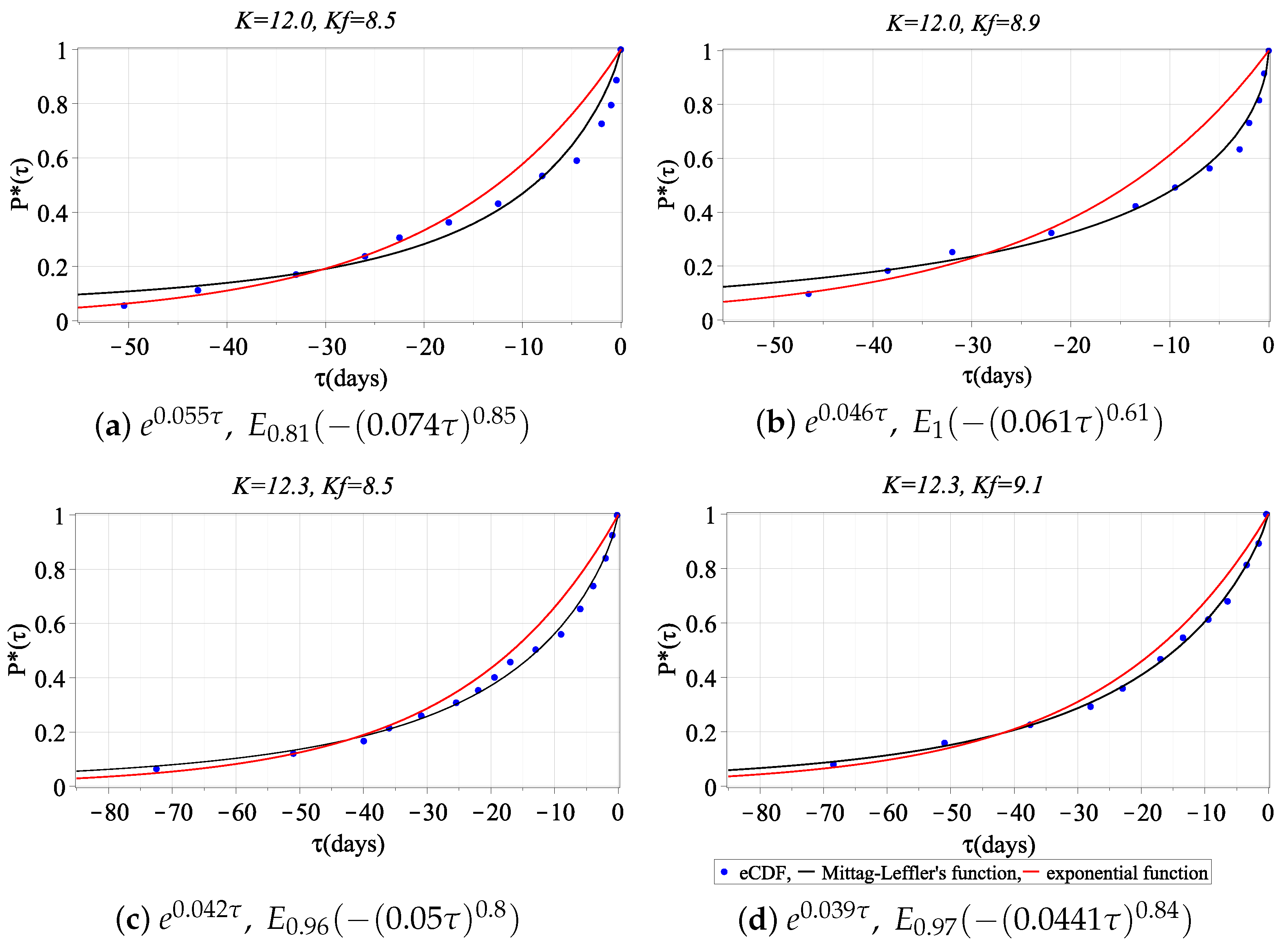
12.0	8.5	$e^{\mu \tau }$	0.113	12.56	0.055
		$E_{\nu }(-{\left(\tilde{\mu }\tau \right)}^{\tilde{\nu }})$	0.031	7.33	0.074	0.81	0.85
12.0	8.9	$e^{\mu \tau }$	0.183	17.27	0.046
		$E_{\nu }(-{\left(\tilde{\mu }\tau \right)}^{\tilde{\nu }})$	0.011	7.14	0.061	1	0.61
12.3	8.5	$e^{\mu \tau }$	0.064	11.1	0.042
		$E_{\nu }(-{\left(\tilde{\mu }\tau \right)}^{\tilde{\nu }})$	0.006	5.03	0.05	0.96	0.8
12.3	9.1	$e^{\mu \tau }$	0.033	9.97	0.039
		$E_{\nu }(-{\left(\tilde{\mu }\tau \right)}^{\tilde{\nu }})$	0.003	3.55	0.044	0.97	0.84
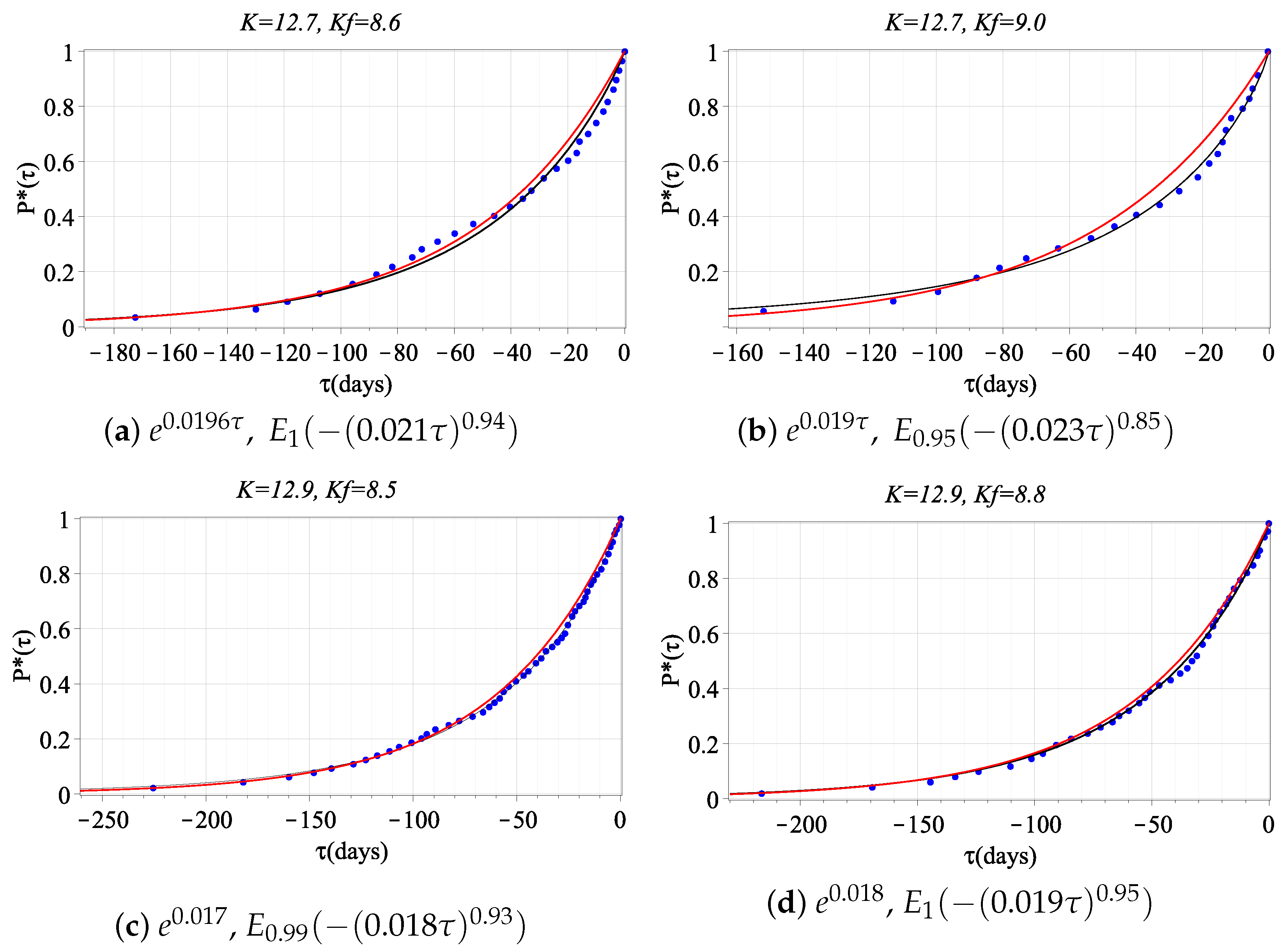
12.7	8.6	$e^{\mu \tau }$	0.057	7.27	0.0196
		$E_{\nu }(-{\left(\tilde{\mu }\tau \right)}^{\tilde{\nu }})$	0.033	6.84	0.021	1	0.94
12.7	9.0	$e^{\mu \tau }$	0.069	9.35	0.02
		$E_{\nu }(-{\left(\tilde{\mu }\tau \right)}^{\tilde{\nu }})$	0.01	6.58	0.023	0.95	0.85
12.9	8.5	$e^{\mu \tau }$	0.023	3.9	0.017
		$E_{\nu }(-{\left(\tilde{\mu }\tau \right)}^{\tilde{\nu }})$	0.004	3.6	0.018	0.99	0.93
12.9	8.8	$e^{\mu \tau }$	0.013	2.94	0.018
		$E_{\nu }(-{\left(\tilde{\mu }\tau \right)}^{\tilde{\nu }})$	0.008	3.91	0.019	1	0.95
12.9	9.0	$e^{\mu \tau }$	0.022	6.54	0.017
		$E_{\nu }(-{\left(\tilde{\mu }\tau \right)}^{\tilde{\nu }})$	0.022	6.54	0.017	1	1
12.9	9.8	$e^{\mu \tau }$	0.054	9.23	0.017
		$E_{\nu }(-{\left(\tilde{\mu }\tau \right)}^{\tilde{\nu }})$	0.006	2.72	0.019	0.99	0.87

and in Figure 5 and Figure 6. The comparison of the approximation results by the Mittag–Leffler function and the exponential function showed the better accuracy of the Mittag-Leffler function (Table 2). The approximation error for the Mittag-Leffler function is units of percent. As a rule, it is much smaller than the approximation error of the exponential function, except in cases where the exponential function is the best approximation ($\nu ={\nu }^{\prime }=1$).

The value of the average density $\tilde{\mu }$ of the event stream in a deformation perturbation is of the order of ${10}^{-2}$ when the empirical laws $P^{*}\left(\tau \right)$ are approximated by the function (4). This coincides with the estimate obtained from the catalog. It is necessary to note that eCDF has its best approximation by the Mittag–Leffler function with close or equal values of the parameters $\nu$ and $\tilde{\nu }$. This possibly indicates the relationship of non-local processes in time (hereditarity) and in space. In addition, if the energy class of the mainshock (Figure 5) is decreased, then the parameter values $\nu$, $\tilde{\nu }$ are decreased, and the value $\tilde{\mu }$ is increased. We observe the opposite situation when the class of the mainshock is increased (Figure 6).

5. Conclusions

In this paper, the fractional Poisson process is used to describe irreversible deformation changes. The deformation process is considered from a probabilistic point of view as a transition from one state (or mode) to another. The fractional Mittag–Leffler function, which takes into account the properties of non-locality (i.e., history of the process), were used to describe the modes of the deformation process. The proposed model is a logical continuation and extension of the Poisson process model with independent events. In addition, the fractional parameters $\nu$ and $\tilde{\nu }$ are determined by the medium parameters, which makes possible a more complete description of its properties.

At the present time, the regularities in the sequences of aftershocks are well researched. In this article, based on the criteria related to the energy and characteristics of the medium of the earthquake preparation area, sequences of foreshocks (clusters) are constructed. The eCDFs of the foreshock waiting time depending on the time before the mainshock are obtained.

The variation of the fractional parameters $\nu$, $\tilde{\nu }$ and the scale factor $\tilde{\mu }$ of the Mittag–Leffler function makes possibility to approximate eCDF $P^{*}\left(\tau \right)$ with it. The approximation of statistical results using the Mittag–Leffler function showed that the accuracy of the approximation by this function is higher than the approximation using the exponential function. The best approximation of the eCDF $P^{*}\left(\tau \right)$ was obtained for close values of the parameters $\nu$ and $\tilde{\nu }$ of the Mittag–Leffler function. There are differences in the behavior of foreshocks for weak and strong mainshocks. This can be interpreted as a difference in the memory effects of events of different energies. It should be noted that due to the small amounts of data, seismology is not statistically sufficient to strictly solve the problem of choosing a deformation model in favor of the fractional Poisson process. However, it remains preferable due to its universal nature.

This model can be useful in the study of induced seismicity, in which the patterns are most likely the same as in natural seismicity. Induced seismicity has an important applied value associated with the injection of fluid into wells during oil refining [29,30,31].

References

- Mogi, K. Active periods in the world’s shieft seismic belts. Tectonophysics 1974, 22, 265–282. [Google Scholar] [CrossRef]
- Kagan, Y.; Knopoff, L. Earthquake risk prediction as a stochastic process. Phys. Earth Planet. Inter. 1977, 14, 97–108. [Google Scholar] [CrossRef]
- Bak, P.; Christensen, K.; Danon, L.; Scanlon, T. Unified scaling law for earthquakes. Phys. Rev. Lett. 2002, 88, 178501-1–178501-4. [Google Scholar] [CrossRef] [PubMed] [Green Version]
- Keilis-Borok, V.I.; Soloviev, A.A. Nonlinear Dynamics of the Lithosphere and Earthquake Prediction; Springer: Berlin/Heidelberg, Germany, 2003; p. 337. [Google Scholar]
- Zaliapin, I.; Gabrielov, A.; Keilis-Borok, V.; Wong, H. Clustering Analysis of Seismicity and Aftershock Identification. Phys. Rev. Lett. 2008, 101, 018501. [Google Scholar] [CrossRef] [PubMed] [Green Version]
- Pisarenko, V.F.; Rodkin, M.V. Declustering of Seismicity Flow: Statistical Analysis. Izv. Phys. Solid Earth 2019, 55, 733–745. [Google Scholar] [CrossRef]
- Zaliapin, I.; Ben-Zion, Y. Earthquake declustering using the nearest-neighbor approach in space-time-magnitude domain. J. Geophys. Res. Solid Earth 2020, 125, 1–33. [Google Scholar] [CrossRef]
- Manna, S.S. Two-state model of self-organized criticality. J. Phys. A Math. Gen. 1991, 24, L363–L369. [Google Scholar] [CrossRef]
- Shebalin, P.N. Increased correlation range of seismicity before large events manifested by earthquake chains. Tectonophysics 2006, 424, 335–349. [Google Scholar] [CrossRef]
- Shebalin, P.; Narteau, C. Depth Dependent Stress Revealed by Aftershocks. Nat. Commun. 2017, 8, 1317–1318. [Google Scholar] [CrossRef] [Green Version]
- Shebalin, P.N.; Narteau, C.; Baranov, S.V. Earthquake Productivity Law. Geophys. J. Int. 2020, 222, 1264–1269. [Google Scholar] [CrossRef]
- Shevtsov, B.M.; Sagitova, R.N. A diffusion approach to the statistical analysis of Kamchatka seismicity. J. Volcanol. Seismol. 2012, 6, 116–125. [Google Scholar] [CrossRef]
- Shevtsov, B.M.; Sagitova, R.N. Statistical analysis of seismic processes on the basis of the diffusion approach. Dokl. Earth Sci. 2009, 426, 642–644. [Google Scholar] [CrossRef]
- Baiesi, M.; Paczuski, M. Complex networks of earthquakes and aftershocks. Nonlinear Process. Geophys. 2005, 12, 1–11. [Google Scholar] [CrossRef]
- Davy, P.; Sornette, A.; Sornette, D. Some consequences of a proposed fractal nature of continental faulting. Nature 1990, 348, 56–58. [Google Scholar] [CrossRef]
- Kagan, Y.Y.; Knopoff, L. Spatial distribution of earthquakes: The two-point correlation function. Geophys. J. R. Astr. Soc. 1980, 62, 303–320. [Google Scholar] [CrossRef] [Green Version]
- Saichev, A.I.; Zaslavsky, G.M. Fractional kinetic equations: Solutions and applications. Chaos 1997, 7, 753–764. [Google Scholar] [CrossRef] [PubMed] [Green Version]
- Carbone, V.; Sorriso-Valvo, L.; Harabaglia, P.; Guerra, I. Unified scaling law for waiting times between seismic events. Europhys. Lett. 2005, 6, 1036–1042. [Google Scholar] [CrossRef]
- Kagan, Y.Y. Observational evidence for earthquakes as nonlinear dynamic process. Phys. D 1994, 77, 160–192. [Google Scholar] [CrossRef]
- Metzler, R.; Klafter, J. The random walk’s guide to anomalous diffusion: A fractional dynamics approach. Phys. Rep. 2000, 339, 1–77. [Google Scholar] [CrossRef]
- Turcotte, D. Fractals and Chaos in Geology and Geophysics, 2nd ed.; Cambridge University Press: London, UK, 1997; p. 416. [Google Scholar]
- Shevtsov, B.; Sheremetyeva, O. Fractional models of seismoacoustic and electromagnetic activity. E3S Web Conf. Sol. 2017, 20, 02013. [Google Scholar] [CrossRef] [Green Version]
- The Geophysical Service of the Russian Academy of Sciences. Available online: http://www.gsras.ru/new/eng/catalog/ (accessed on 27 February 2022).
- Fedotov, S.A. Regularities of the distribution of strong earthquakes in Kamchatka, the Kurile Islands, and northeastern Japan. Tr. Inst. Phys. Earth. Acad. Sci. USSR 1965, 36, 66–93. [Google Scholar]
- Laskin, N. Fractional Poisson processes. Commun. Nonlinear Sci. Numer. Simul. 2003, 8, 201–213. [Google Scholar] [CrossRef]
- Uchaikin, V.V. Self-similar anomalous diffusion and stable laws. Phys. Uspekhi 2003, 46, 821–849. [Google Scholar] [CrossRef]
- Dobrovolsky, I.R.; Zubkov, S.I.; Myachkin, V.I. Estimation of the size of earthquake preparation zones. Pure Appl. Geophys. 1979, 117, 1025–1044. [Google Scholar] [CrossRef]
- Davis, J.C. Statistics and Data Analysis in Geology, 2nd ed.; John Wiley and Sons. Inc.: New York, NY, USA, 1986; p. 267. [Google Scholar]
- Broccardo, M.; Mignan, A.; Wiemer, S.; Stojadinovic, B.; Giardini, D. Hierarchical Bayesian Modeling of Fluid-Induced Seismicity. Geophys. Res. Lett. 2017, 44, 11–357. [Google Scholar] [CrossRef] [Green Version]
- Khajehdehi, O.; Eaton, D.W.; Davidsen, J. Spatiotemporal Clustering of Seismicity in the Kiskatinaw Seismic Monitoring and Mitigation Area. Front. Earth Sci. 2022, 10, 894549. [Google Scholar] [CrossRef]
- Vorobieva, I.A.; Gvishiani, A.D.; Dzeboev, B.A.; Dzeranov, B.V.; Barykina, Y.V.; Antipova, A.O. Nearest Neighbor Method for Discriminating Aftershocks and Duplicates When Merging Earthquake Catalogs. Front. Earth Sci. 2022, 10, 820277. [Google Scholar] [CrossRef]