Article

Fractal Properties of the Magnetic Polarity Scale in the Stochastic Hereditary αω-Dynamo Model

by
Gleb Vodinchar 
* and
Lyubov Feshchenko
Institute of Cosmophysical Research and Radio Wave Propagation FEB RAS, 7, Mirnaya Str., Paratunka, 684034 Kamchatka, Russia
*
Author to whom correspondence should be addressed.
Fractal Fract. 2022, 6(6), 328; https://doi.org/10.3390/fractalfract6060328
Submission received: 30 April 2022 / Revised: 5 June 2022 / Accepted: 10 June 2022 / Published: 13 June 2022
(This article belongs to the Special Issue Fractional Calculus and Fractals in Mathematical Physics)

Abstract

:
We study some fractal properties of the hereditary α ω -dynamo model in the two-mode approximation. The phase variables of the model describe the temporal dynamics of the toroidal and poloidal components of the magnetic field. The hereditary operator of the quenching the α -effect by field helicity in numerical simulation is determined using the Riemann–Liouville fractional differentiation operator. The model also includes a stochastic term. The structure of this term corresponds to the effect of coherent structures from small-scale magnetic field and velocity modes. A difference scheme and a program code for numerical simulation have been developed and verified. A series of computational experiments with the model has been carried out. The Hausdorff dimension of the polarity scale in the model and the distribution of polarity intervals are calculated. It is shown that the Hausdorff dimension of the polarity scale is less than 1, i.e., this scale is a fractal. The numerical value of the dimension for some values of the control parameters is 0.87, which is consistent with the dimension of the real geomagnetic polarity scale. The distribution histogram of polarity intervals in the model has a pronounced power-law tail, which also agrees with the properties of real polarity scales.

1. Introduction

The large-scale magnetic fields exist in space objects of various spatial scales—galaxies, planets, stars. All these fields are formed and maintained at a fairly stable level by a single physical mechanism—a hydromagnetic dynamo [1]. The main method for studying cosmic dynamo systems is modeling, since it is impossible to reproduce in laboratories the values of the dimensionless parameters of the Reynolds number Re and the Reynolds magnetic number Rm , which are typical for cosmic media.
Briefly, the idea of a dynamo is in the following [1]. Let at the initial moment of time the conducting medium be weakly magnetized by some external magnetic field. Then the movement of such media can, under certain conditions, lead to the formation of a new magnetic field, which is much larger than the original one. This field, in turn, influences the motion of the medium, correcting the generation process. Feedback arises, leading to the generation of a field of finite magnitude. Since the magnetic field has zero divergence, it is always possible to distinguish between toroidal and poloidal components in it. In the cycle of dynamo work, these two components mutually generate each other.
The dynamo equations are quadratic in the magnetic field, which always makes it possible to have symmetric solutions, i.e., no preferred field polarity. It also gives the possibility of reversals—quick changes in the polarity of the field. These reversals are observed in real dynamo systems [2,3].
In general, such systems are characterized by different dynamic regimes. Regular and chaotic oscillations, vacillations, bursts, excursions (short changes in polarity after which the polarity is restored) are observed. Therefore, we can say that cosmic dynamo systems are complex oscillatory systems.
In dynamo theory, it is established that field generation is impossible under conditions of axial symmetry. On the other hand, the observed large-scale magnetic fields and media streams are axisymmetric in the first approximation.
Cosmic objects have very large values of Re and Rm . For example, for the Earth Re 10 9 , Rm 10 3 , and for the Sun Re 10 14 , Rm 10 9 . This is a sign of strong turbulence with many spatial scales. Since direct numerical simulation is not possible with such numbers, mean field models are used. In these models, large-scale axis-symmetric fields and three-dimensional small-scale pulsations are distinguished. Then, the dynamo equations are averaged over the fluctuations. The most popular model is α ω -dynamo.
The idea of α ω -dynamo for cosmic magnetic field was proposed by [4]. The main difficulty of this dynamo is in the feedback, when a large-scale magnetic field affects the turbulent generator, providing a self-consistent nonlinear mechanism for generating a finite field. Usually this feedback assumed to be instantaneous in time and local in space. However, the proper description of turbulent transport involves the convolution of integral kernels with the mean field [5]. The authors of [6] showed that the memory effect strongly affects the dynamo action. The [7] used the formalism of response functions and showed that the effect of the integral kernels can be significant for anisotropic flows. Therefore, when modeling a dynamo, it is desirable to take into account this memory (heredity).
One way to build the desired models is as follows. For the fields of velocity and magnetic induction, additive expansions into large-scale modes with time-varying coefficients (amplitudes) are introduced. These expansions are substituted into the dynamo equations and the procedure of the Galerkin method is applied. In order to take into account the memory effect for the mode amplitudes in a dynamic system, it is necessary to introduce hereditary terms in one way or another. In this way, a two-mode model was constructed in [8] where it was shown that the α ω -dynamo can be regarded as an oscillator with a hereditary potential.
If the large-scale spatial structure of the field is sufficiently simple, a small number of modes can be used. As a result, we obtain a low-mode model. The advantage of low-mode models is that they allow calculating the long-term evolution of the magnetic field on the time scales of the space object’s existence—billions of years.
This makes it possible to compare the statistical characteristics of solutions with data on the behavior of the geomagnetic field in the distant past. Information about the temporal evolution of the geomagnetic field is contained in paleomagnetic records that record the residual magnetization of ferromagnetic minerals during their crystallization. Based on these records, geomagnetic polarity timescales (GMPTS) are constructed. It turns out a time series of evolution of a large-scale field, unique in duration, in a real dynamo system. The longest GMPTS covers 1700 Myr [9].
The different GMPTS form a self-similar fractal structures [9,10]. Intervals between the reversals (polarity intervals) differ by several orders of magnitude, there are long intervals without reversals, superchrons [2,11]. Similar fractal properties of solutions were found in various geodynamo models, for example [12,13,14].
In this work, we study one two-mode fractional stochastic hereditary α ω -dynamo model. The phase variables describe the time dynamics of the toroidal and poloidal field components.
The model takes into account the memory effect in the feedback—in the quenching of the turbulent generator by the helicity or energy of the field. The popular way to introduce heredity into mathematical models is to use fractional derivatives [15,16,17]. However, the formal replacement of ordinary differentiation operators in differential models by fractional operators is physically difficult to comprehend. Therefore, in this work, we first introduce the hereditary term in a general form, which is physically well understood, and only then we introduce fractional derivatives for the particular case.
The use of low-mode approximations always assumes that the total effect of discarded small-scale modes is zero. However, in reality, these modes can spontaneously synchronize and have a significant effect on the system. The formation of such coherent structures is well known in the theory of turbulence [18]. Therefore, we introduce into the model a random process that simulates the action of such structures. Previously, we used this approach in one simple model [14].
Note that in this paper we do not consider the reproduction in the model of the complex properties of turbulence, which have been studied in many stochastic dynamo models.
We discuss the fractional differential model of the two-mode dynamo and the fractal properties of the polarity scale, such as the fractional Hausdorff dimension and the power-law distribution of polarity intervals. Moreover, we are trying to introduce fractional operators in the model not formally, but through heredity. Our work is formal mathematical. The possibility of applying its results to specific space objects requires a separate study.
Next, we describe the derivation of the model equations and the difference scheme, simulation results, as well as the statistical properties of the obtained solutions. It turned out that they are in good agreement with the properties of real GMPTS.

2. Hereditary Two-Modes α ω -Dynamo Model

Consider the construction of one hereditary dynamical system, which is one model of a cosmic dynamo-system.
Let an axis-symmetric large-scale magnetic field of a star or planet is generated by large-scale differential rotation and turbulent α -effect. This is the so-called Parker dynamo [4]. We consider that the spatial structure of the field is simple and can be described by one-poloidal and one-toroidal modes.
Then the field generation can be described by the following simple system [8]:
d B T d t = ω B P η T B T , d B P d t = α B T η P B P ,
where B T ( t ) and B P ( t ) have the meaning of the toroidal and poloidal modes amplitudes. Positive constant coefficients: ω is the measure of generation toroidal mode by large-scale differential rotation, α is the measured generation poloidal mode by helicity of small-scale turbulence, 1 / η T and 1 / η P are the character times of modes dissipation. Explicit expressions for these coefficients (Galerkin coefficients) are given in [8] and are not important now.
The model (1) is linear (so-called kinematic dynamo), so the generation of a finite magnetic field is impossible. It is also clear that generation will occur in case D = α ω η T η P > 1 . Exactly in this case the zero equlibrium point will be unstable and the small initial values of the field will increase. Therefore, the dimensionless parameter D is called the relative dynamo number. In what follows, we will call it the dynamo number for short.
In the real physical dynamo system the magnetic field is changes turbulent medium flow by Lorentz force, and the generation of field is quench. In particular, the small-scale turbulence helicity is changes.
We can introducing feedback ( α -quenching) into the (1). The Lorentz force is quadratic in the magnetic field, so the feedback can be introduced into the model in the form:
α α 1 w ( t ) ,
where α is the helicity in the absence of a strong magnetic field, and w ( t ) is dimensionless dynamical correction. This correction is quadratic expressed in terms of B T ( t ) and B P ( t ) .
In the simplest case w ( t ) = Q B T ( t ) , B P ( t ) , where Q ( · , · ) is a quadratic form. Such type models are known as algebraic quenching models [1,19,20].
In more complex models, an evolution equation (dynamical quenching) is introduced for w ( t ) in the form:
D w ( t ) = Q B T ( t ) , B P ( t ) ,
where D is some differential operator [21,22].
A more general form of dynamical quenching is obtained by defining w ( t ) as t-parametric functional [8,23]:
w ( t ) = 1 t K B 0 2 0 t K t τ t K Q B T ( τ ) , B P ( τ ) d τ ,
where K ( · ) is some dimensionless kernel, with the properties K ( 0 ) 0 and K ( + ) = 0 , t K is the time scale of kernel, B 0 is some typical value of field. This predetermined expression specifies the model of hereditary quenching. This is a memory model. Obviously, if we change the kernel K by a constant factor c > 0 , this is equivalent to changing B 0 by the factor c . Therefore, in what follows, we always consider the kernel K in a normalized suitable way.
Two special cases of form Q B T ( t ) , B P ( t ) have an obvious physical meaning. In the first case Q = | B T ( t ) | 2 + | B P ( t ) | 2 determined field energy. In the second case Q = B T ( t ) B P ( t ) determined field helicity. More generally,
Q = γ | B T ( t ) | 2 + | B P ( t ) | 2 + 1 γ B T ( t ) B P ( t ) , 0 γ 1 .
It must be said that the α -quenching models listed above, with an arbitrary quadratic form Q, have an abstract mathematical character. Most of the works mentioned above use energy as a form Q. It is known that for a strong large-scale field, α B 2 [1]. In addition, the magnetic helicity in reality does not keep up with the changes in the large-scale magnetic field. Helicity cannot be given by an algebraic expression for the large-scale field components. It is determined by the differential equation on the right side of the large-scale field [24,25,26].
However, we will consider the general expression (5) as a mathematical generalization of the models. It will be shown below that this type of form allows one to obtain the Lorenz system as a special case. This classical system was used as a simple model for the chaotic component of the Solar cycle [21].
Now let us make the model ((1), (2), (4)) dimensionless. We will use the diffusion time of the poloidal field 1 / η P as the time scale. Let us now turn to new dimensionless variables (keep the notation for time):
t η P t , B T = B 0 η P α t K x ( t ) , B P = B 0 η T η P ω α t K y ( t ) , w = η T η P α ω z ( t ) ,
and to the new dimensionless parameters:
D = α ω η T η P , μ = η T η P , r = ω η T , p = t K η P .
For these parameters: D is the dynamo-number; μ 1 is the dimensionless time of toroidal field decay; r is the ratio of toroidal and poloidal modes scales; p is the dimensionless time scale of the kernel.
Then the dimensionless model of a two-modes dynamo with memory takes the form:
d x d t = μ ( y x ) , d y d t = ( D z ) x y , z ( t ) = 0 t K t τ p q r , γ x ( τ ) , y ( τ ) d τ ,
where dimensionless quadratic form,
q r , γ x ( τ ) , y ( τ ) = γ r x 2 ( τ ) + 1 r y 2 ( τ ) + 1 γ x ( τ ) y ( τ ) .
We shall also study the case of a <<working dynamo>>, i.e., D > 1 .
The hereditary model of α ω -dynamo (6) and (7) with q r , γ x ( τ ) , y ( τ ) = x ( τ ) y ( τ ) , i.e., γ = 0 was studied in [8]. It was shown that the model can be considered as an oscillator with a hereditary potential.
We can highlight two particular cases of the kernel. In the first case, the kernel is a power function of the form K ( s ) = s β Γ ( 1 β ) , 0 < β < 1 . Then, differentiating third equation of system (6) with respect to time t, we get:
d z d t = p β Γ ( 1 β ) · d d t 0 t q r , γ x ( τ ) , y ( τ ) t τ β d τ = p β D 0 + β q r , γ x ( t ) , y ( t ) ,
where D 0 + β is the Riemann–Liouville fractional derivative operator of order β .
So, the dynamo model in this case is the system of fractional differential equations:
d x d t = μ y x , d y d t = D z x y , d z d t = p β D 0 + β q r , γ x , y , z ( 0 ) = 0 .
In the second particular case (for a whole class of kernels), the dynamo model can be written as a classical differential system. Let the kernel be a solution of a linear homogeneous differential equation of order n with constant coefficients:
a n K ( n ) ( t ) + a n 1 K ( n 1 ) ( t ) + + a 1 K ( t ) + a 0 K ( t ) = 0 .
Then, the third equation of system (6) is equivalent to differential Equation (8):
k = 0 n a k p k d k z d t k = k = 0 n a k m = 0 k 1 p k m K ( m ) ( 0 ) d k m 1 d t k m 1 q r , γ x , y ,
with initial conditions
z ( 0 ) = 0 , z ( m ) ( 0 ) = k = 0 m 1 K ( m k 1 ) ( 0 ) d k d t k q r , γ x ( t ) , y ( t ) | t = 0 , m = 1 , , n 1 .
Therefore, the integro-differential system (6) can be specified using the l-th order differential system, where 3 l 3 n 2 . The order l of this system depends on the initial conditions for the kernel K and its derivatives.
Note that arbitrary initial conditions can only be chosen for variables x and y. The rest of the initial conditions will be determined from (12), first, and second system (6) equations. Therefore, the phase space of the model will be only some manifold in the space of variables x , y , z , z , , z ( n 1 ) .

3. Stochastic α ω -Dynamo Model

Let us now introduce into the model the stochastic term ξ ( t ) , which describes the influence of coherent structures, spontaneously formed by small-scale magnetic modes. Depending on the morphology of each structure, it can either enhance or weaken the field generation. Therefore, this term we introduce into the model as an additive correction to the dynamo number. The mean of this correction should be zero.
Now, we the model structure of this process describe. We assume that the k-th coherent structure spontaneously forms at random time φ k and self-destructs at random time θ k . We neglect the possibility of the simultaneous existence of two or more coherent structures. Therefore, we have the stochastic increasing sequence of time points: 0 < φ 1 < θ 1 < φ 2 < θ 2 < < φ k < θ k < .
Then, τ k W = φ k θ k 1 is a random waiting time for the k-th structure to formation, and τ k E = θ k φ k is a random time for the structure existence.
Let the random variables ξ k with zero mean describe the intensity of the k-th structure influence on the field generation. Intensities ξ k are independent and identically distributed Gaussian random variables: ξ k N ( 0 , σ 2 ) .
The emergence of coherent structures is quite rare, and they exist for a short time. Therefore, it is reasonable to assume in the model that the distribution asymptotic properties for a waiting time and for an existence time should be very different. Therefore, we will assume that the variables τ k W are power-law distributed with the T W typical value, and the variables τ k E are exponential law distributed with the T E typical value. Since the mean of a power-law distribution can be infinite, we will use the median of the distribution as a typical value.
So, we take the probability density function (pdf) for the waiting time in the form:
p W ( t ) = ν 1 c T W 1 + t c T W ν , c = 2 1 ν 1 1 1 , ν > 1 , t 0 ,
and we take the pdf for the existing time in the form:
p E ( t ) = ln 2 T E exp ln 2 T E t , t 0 .
Random variables with such distributions can be easily simulated using the inversion method:
τ E = T E ln 2 ln U and τ W = c T W U 1 / ( 1 ν ) 1 ,
where random variable U is uniform on 0 ; 1 .
All random variables ξ k , τ k W and τ k E are assumed to be independent for different k and of each other.
Now we define the process ξ ( t ) as follows:
ξ ( t ) = k = 1 + ξ k H ( t τ k ) H ( t θ k ) ,
where H ( · ) is Heaviside step function.
So, the stochastic hereditary α ω -dynamo model is defined by the following equations:
d x d t = μ ( y x ) , d y d t = ( D + ξ ( t ) z ) x y , z ( t ) = 0 t K t τ p q r , γ x ( τ ) , y ( τ ) d τ .
The model is closed by the initial conditions x ( 0 ) = x 0 , y ( 0 ) = y 0 .
Let us now find the equilibrium points x * , y * , z * of the model (17).
To do this, we solve the system:
μ ( y * x * ) = 0 , D + ξ ( t ) z * x * y * = 0 , z * = q r , γ x * , y * 0 t K t τ p d τ .
Clearly x * = y * = z * = 0 is the solution and anyway x * = y * . We then obtain from the second equation, that D + ξ ( t ) z * 1 x * = 0 . If x * 0 , then z * = D + ξ ( t ) 1 . Since ξ ( t ) varies with time and z * is constant, this equality is impossible. So, the model (17) has only zero equlibrium point.
Now we will determine the stability of this point. To do this, note that in system (17) there are only two phase variables actually— x ( t ) and y ( t ). The variable z ( t ) is just a notation for the integral term. Therefore, we consider system (17) as two-dimensional. Then the elements of the Jacobi matrix:
J 11 = μ , J 12 = μ , J 21 = x 0 t K t τ p x q r , γ x ( τ ) , y ( τ ) d τ + + D + ξ 0 t K t τ p q r , γ x ( τ ) , y ( τ ) d τ , J 22 = x 0 t K t τ p y q r , γ x ( τ ) , y ( τ ) d τ 1 .
It can be seen that at the equilibrium point ( 0 ; 0 ) : J 11 = μ , J 12 = μ , J 21 = D + ξ , J 22 = 1 . We then find the characteristic equation and use the Routh–Hurwitz criteria to determine its stability. The equilibrium point ( 0 ; 0 ) turns out to be stable if D + ξ ( t ) < 1 and unstable if D + ξ ( t ) > 1 .

4. Difference Scheme for Model
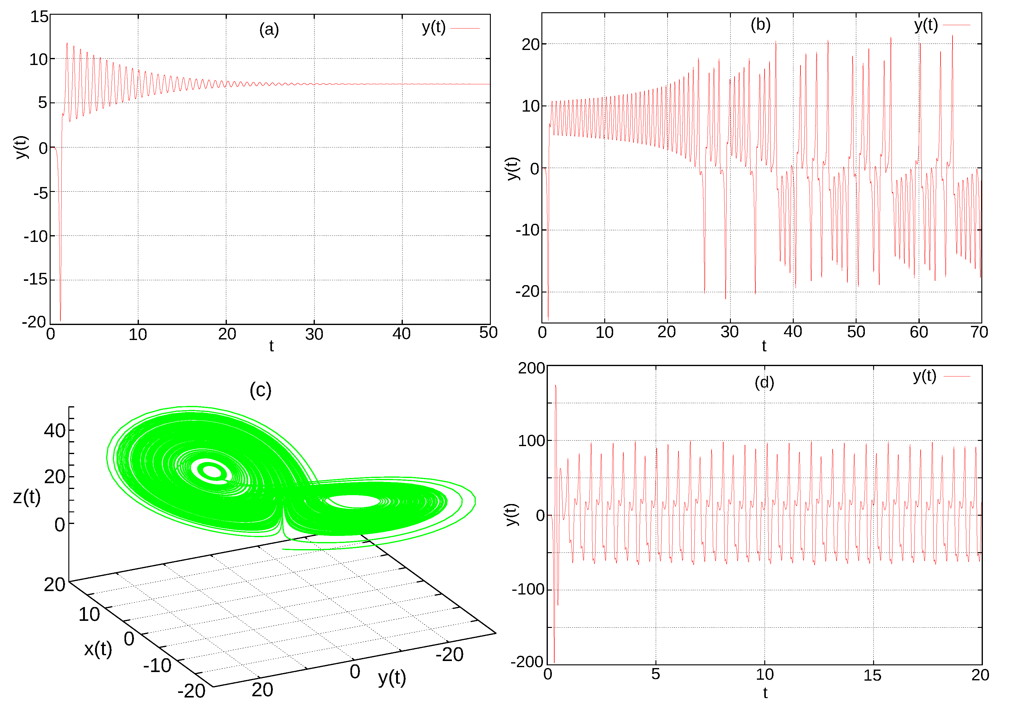
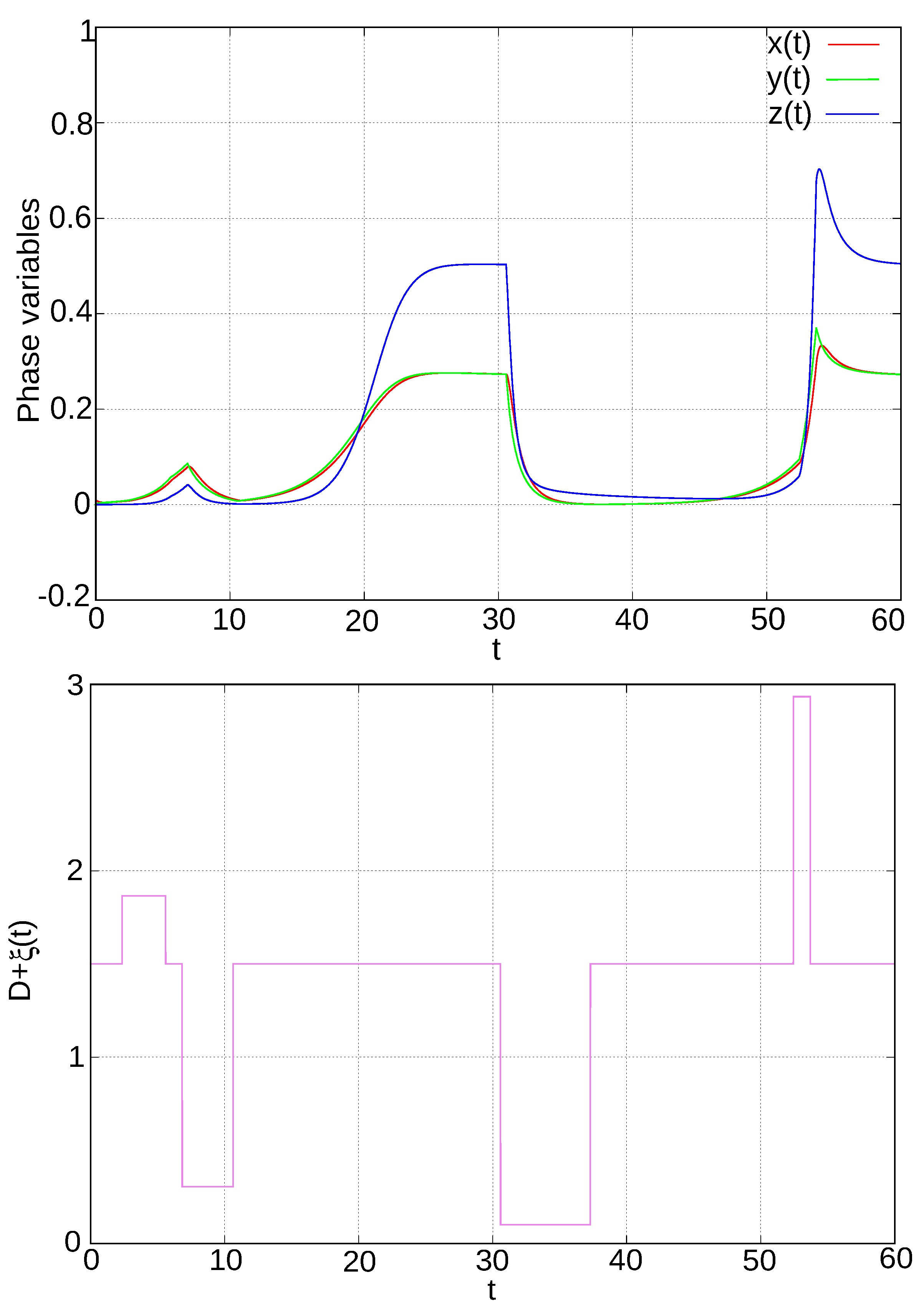
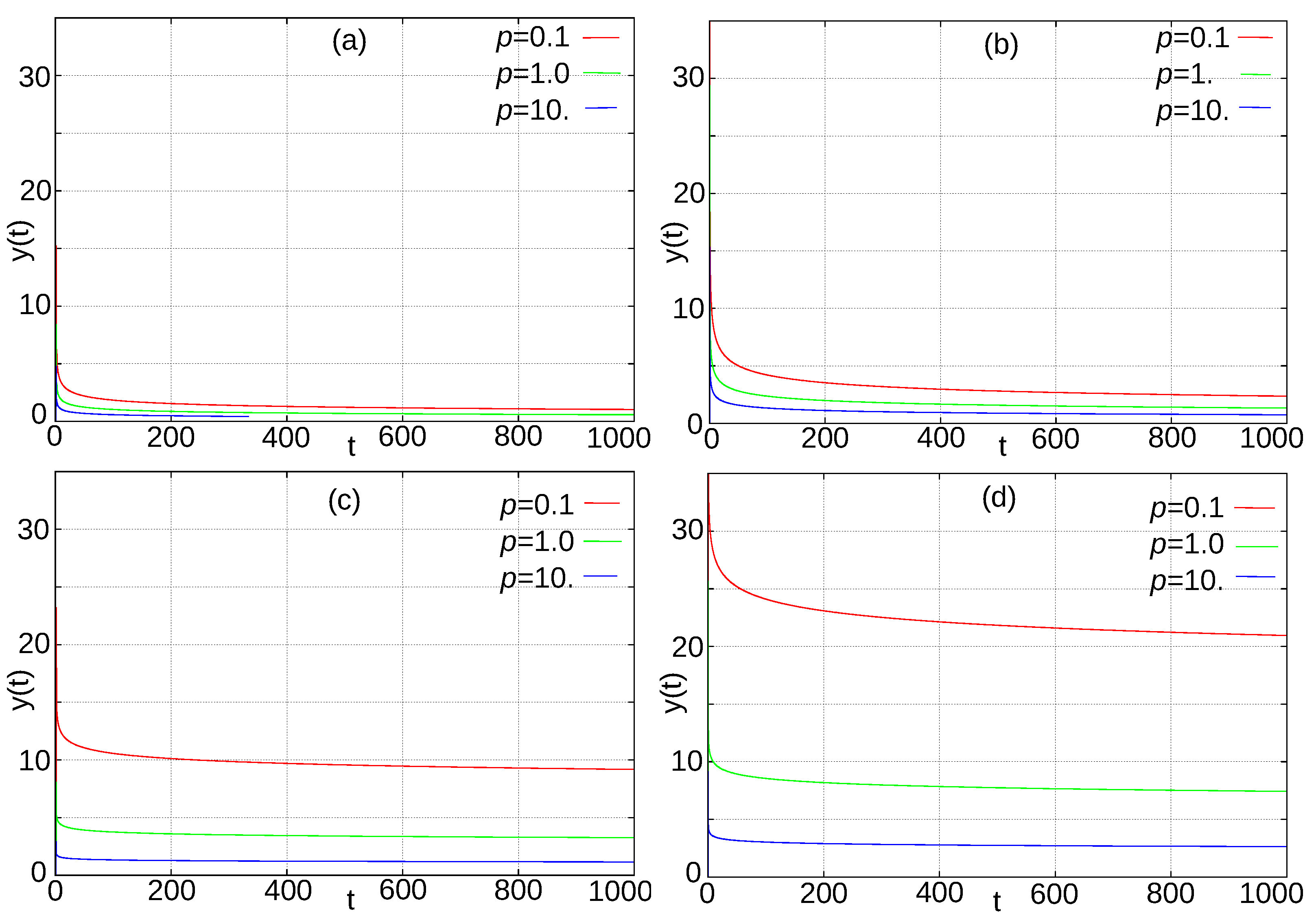
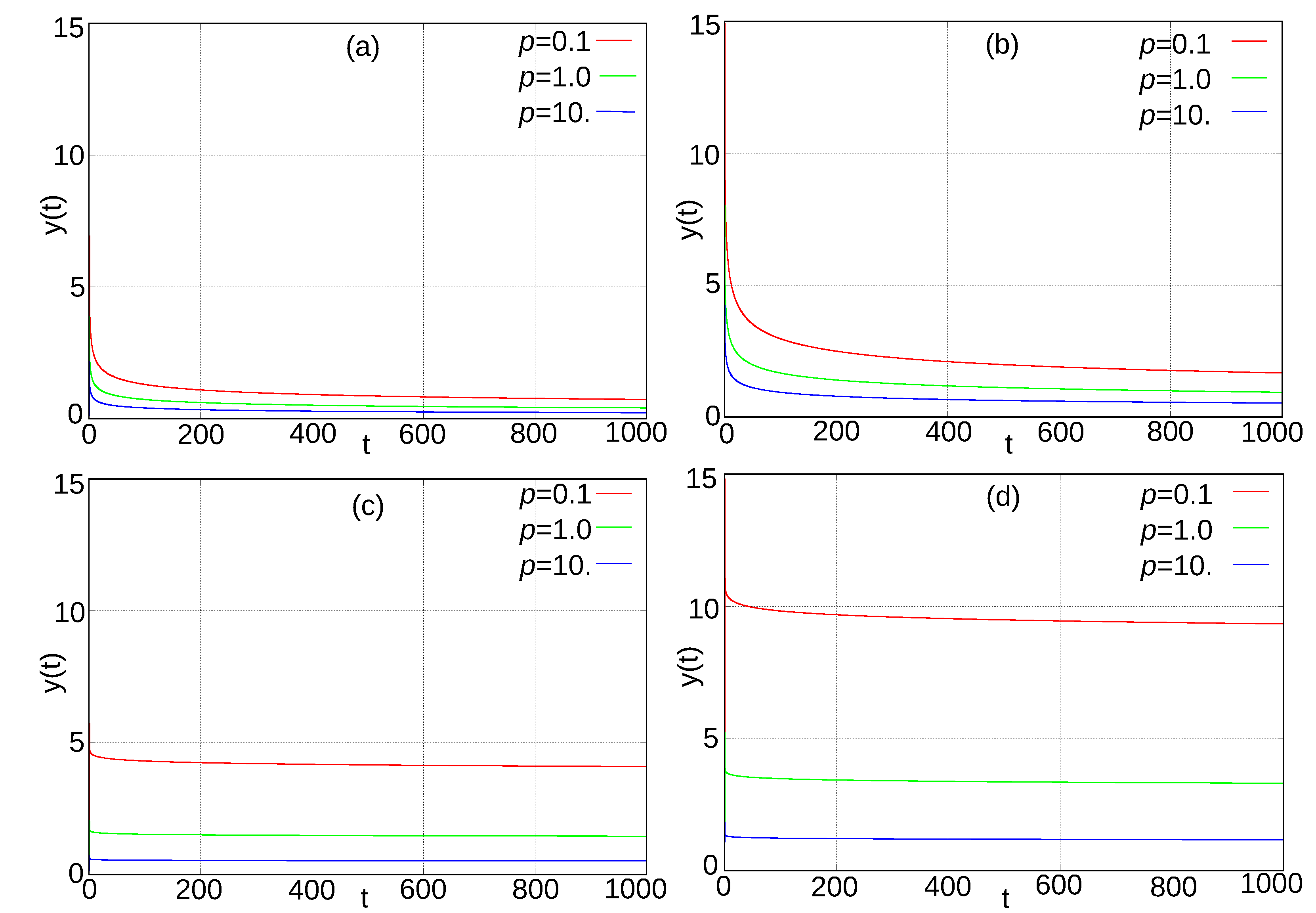
We introduce the time step h and uniform time grid t n = n h . The corresponding values of the phase variables x n , y n and z n . We also denote K n = K n h p and q n = q r , γ x n , y n .
For the integral part (third equation) of the system (17), we will use the Simpson’s rule:
z n + 1 = L + h 3 K 0 q n + 1 = L + h 3 K 0 q r , γ x n + 1 , y n + 1 ,
where for even n:
L = 2 h 3 2 K 1 q n + K 2 q n 1 + 2 K 3 q n 2 + + K n q 1 + 2 K n + 1 q 0 ,
and for odd n:
L = 2 h 3 2 K 1 q n + K 2 q n 1 + 2 K 3 q n 2 + + 2 K n q 1 + K n + 1 q 0 .
These expressions use non-local boundary conditions: x ( 0 ) = x 0 , y ( 0 ) = y 0 , and x ( < 0 ) = y ( < 0 ) = 0 .
For the first and second equations (differential part) of the system (17) we use the trapezoidal rule (implicit second-order Runge–Kutta method [27]):
x n + 1 = x n + h 2 μ y n x n + μ y n + 1 x n + 1 , y n + 1 = y n + h 2 D + ξ n z n x n y n + D + ξ n + 1 z n + 1 x n + 1 y n + 1 .
Now we combine (20)–(23) together into one system, and we get an implicit non-local difference scheme for numerical simulation:
x n + 1 = x n + h 2 μ y n x n + μ y n + 1 x n + 1 , y n + 1 = y n + h 2 D + ξ n z n x n y n + D + ξ n + 1 z n + 1 x n + 1 y n + 1 , z n + 1 = i = 0 n + 1 ϕ n i K n + 1 i q r , γ x i , y i ,
where ϕ n i are defined by (20)–(22).
We determine the equilibrium points of the numerical scheme (24) by setting x n + 1 = x n = = x 0 = x * and similarly for y and z. We get a system:
2 μ y * x * = 0 , 2 D x * 2 y * z * x * + ξ n + ξ n + 1 x * = 0 , z * = q r , γ x * , y * i = 0 n + 1 ϕ n i K n + 1 i .
We obtain that x * = y * . Then the second equation gives two cases. In the first case x * = y * = 0 , then z * = 0 from the third equation. In the second case 2 D 2 z * + ξ n + ξ n + 1 = 0 , which is impossible with a time-varying random process ξ ( t n ) .
So, scheme (24) has zero equilibrium point, as well as model (17). The scheme is implicit with cubic non-linearity. Therefore, it is very difficult to study the stability of the equilibrium point by analytical methods. We found out with the help of numerical experiments that the point of stability conditions for the equilibrium point are the same as for the model (17). The results of these experiments are described below in the paper.
We then transform the scheme (24) to simplify the calculations.
Note that from the first Equation (23) it is easy to explicitly express x n + 1 and in terms of x n , y n , and y n + 1 :
x n + 1 = h μ 2 + h μ y n + 1 + 2 x n + h μ y n x n 2 + h μ .
Substituting this expression instead of x n + 1 in (20) and in second Equation (23), we get only one nonlinear equation with the unknown y n + 1 :
a 0 + a 1 y n + 1 + a 2 y n + 1 2 a 3 y n + 1 3 = 0 .
Expressions for the coefficients a i are given in the Appendix A. We solve this equation by Newton’s method using y n as an initial guess for y n + 1 . Then, we calculate x n + 1 , q n + 1 and z n + 1 :
x n + 1 = h μ 2 + h μ y n + 1 + 2 x n + h μ y n x n 2 + h μ , q n + 1 = q r , γ x n + 1 , y n + 1 , z n + 1 = h 3 K 0 q n + 1 + L .
This modified form (27) and (28) of the difference scheme (24) was programmed in C++ code. The main part of this code is given in the Appendix B.
We studied the stability of the zero equilibrium point in a series of computational experiments by varying the model parameters and the type of kernel. At the initial stages of simulation, it always turned out that for D + ξ ( t ) < 1 the phase trajectories approached zero. If the phase variables are small and D + ξ ( t ) > 1 , then the growth begins. This is in full agreement with the equilibrium point stability criteria in the model (17). This response was very fast at the beginning of the simulation and gradually slowed down with increasing time. This is a manifestation of memory in the system.
A typical result is shown in Figure 1. The calculations were carried out for the kernel K ( s ) = s β / Γ ( 1 β ) corresponding to the order β fractional derivative operator. You can see the fast response of the phase variables to a change of D + ξ ( t ) for t 25 . Next comes the fast response to a negative outlier in ξ ( t ) 5 at t 31 . However, the reaction to switching ξ ( t ) at t 38 is already much slower.
To verify the C++ code, we carried out simulation for kernel K ( s ) = exp ( s ) and for γ = 0 , σ = 0 . In this case, the system (17) will not be stochastic, since ξ ( t ) 0 . However, the program must correctly resolve the system.
In this case, Equation (11) will take the form d z d t = x y 1 p z , process ξ ( t ) 0 , and the dynamo model (17) will be equivalent to the system:
d x d t = μ ( y x ) , d y d t = ( D z ) x y , d z d t = x y 1 p z , z ( 0 ) = 0 .
This is the classical Lorenz system [28], the dynamics of which at μ = 10 and p = 3 / 8 is well studied [29,30]. Therefore, if the difference scheme and the C++ code work correctly, they should reproduce the known regimes.
Note that the Lorenz system as the simplest model of the Solar α ω -dynamo was proposed in the work [21], and as the model of disk dynamo was used in the work [22].
The simulation results are shown in Figure 2. Three typical regimes for the Lorenz system are shown: asymptotically stationary regime (Figure 2a), chaotic regime (Figure 2b,c), quasi-periodic regime (Figure 2d). It can be concluded that the difference scheme and the program code are working correctly.
Figure 3 shows the simulation results with the same system, but with process ξ ( t ) influence. The processes parameters are given in the figure caption. The dynamics of the field poloidal component y ( t ) and process ξ ( t ) are shown. It can be seen that the system quickly responds to random perturbations.
An important remark needs to be made. On Figure 2a it can be seen that the phase variables asymptotically approach some constant values. A similar situation can be seen in Figure 1 at 25 < t < 30 and t > 65 . How does this correlate with the fact that the model does not have nonzero equilibrium points? The reason is that not all of the x , y , z -space is the phase space of the model.
For example, it is well known that the Lorenz system (29) at D > 1 has two equilibrium points
± ( D 1 ) / p , ± ( D 1 ) / p , D 1 .
However, for K ( s ) = exp ( s ) , the model is equivalent to the Lorenz system together with the initial condition z ( 0 ) = 0 . Therefore, this points are <<punctured>> from the phase space of the model. Lower <<puncture>> points can also occur with other kernels, and these points may turn out to be centers of attraction for phase trajectories. However, it is not possible to determine them in the general case.

5. Fractional Stochastic α ω -Dynamo Model–Simulation Results

Further in the work, we will consider the case of a power kernel K ( s ) = s β Γ ( 1 β ) , 0 < β < 1 , which corresponds to the fractional model. Taking into account the random effect of coherent structures, the model has the form:
d x d t = μ y x , d y d t = D + ξ ( t ) z x y , d z d t = p β D 0 + β q r , γ ( x , y ) , z ( 0 ) = 0 .
We will consider two parameter γ values. In the first case, γ = 0 and α -quenching is provided by the field helicity. In the second case γ = 1 . Then the α -quenching is provided by the field energy.
It is known that if we take one toroidal and one poloidal modes of free decay of a magnetic field with the same spatial scales, the poloidal mode has a smaller eigenvalue [31]. Therefore, we consider that μ > 1 . For the classic Parker’s dynamo [4], for example, the work [31], the results give the values μ 3.37 . It is this value that we will further use in numerical simulation.
For planetary and stellar dynamo systems it is reasonable to assume that x 0 = 0 and | y 0 | 1 . This is related to the fact that a small external field, which is poloidal, is required to start the dynamo system at the initial moment [1]. Therefore, further everywhere x 0 = 0 and y 0 = 10 3 . We also recall that the difference scheme implicitly assumes that the non-local conditions x ( < 0 ) = y ( < 0 ) = 0 .
Such conditions are plausible from the physical point of view. At t < 0 there are no magnetic fields, the dynamo system is in the zero state. At t = 0 , a weak poloidal field arises. It has some external source. Then the dynamo system starts. We will always show the dynamics of y ( t ) in the figures, since only the poloidal component of the field can be observed in real space dynamo systems. The toroidal component of the magnetic field does not have a radial projection, so it is always hidden inside the field generation area (in the core of a planet or in the star convective zone). Therefore, its dynamics can be discussed only on the basis of indirect data.
The model (30) contains many parameters. It was said above that we fixed μ = 3.37 . There are three more parameters in dynamic equations: D > 1 , p > 0 , and β 0 ; 1 . First of all, we determined what these parameters affect, using set numerical simulations for σ = 0 . Thus, we excluded the influence of the random process ξ ( t ) .
It turned out that when varying the parameters D, p, β the dynamical regimes have a similar appearance. The magnetic field without reversals reaches a stationary value. The parameters affect only the magnitude of this stationary value and the time of the transition process. Several typical results are shown in the Figure 4 and Figure 5. It can be seen that an increase in the dynamo number D and fractional derivative order β leads to an increase in the field level. Increasing the scale p, on the contrary, reduces the field level. This pattern was observed in all computational experiments. Simulations were carried out for dynamo numbers up to 10 3 .
The field level is lower for the same values of the parameters with quenching by energy, than with quenching by helicity. Apparently, this is due to the fact that the sign-positive quadratic form leads to greater α -quenching.
Then, for the model (30), obtaining reversals is possible only with the help of a random process.
Note that, earlier, one of the authors of this paper studied a similar model (without random disturbances) with other types of power kernels, that are not related to fractional differentiation [8]. More complex dynamic regimes were discovered: quasi-regular and chaotic oscillations and vacillations, dynamo bursts. These regimes arose for dynamo number D 200 .
For the Earth’s core, the product of the dimensionless intensities of the α - and ω -effects in less than an order of magnitude exceeds the field generation threshold [32,33]. In the model (30), the generation threshold: D = 1 . Therefore, in numerical simulations, we always take the value D = 8 .
In this work, we were interested in the possibility of reproducing such properties of a real GMPTS as a fractional dimension and a power-law distribution of field polarity intervals.
Next, we consider the simulation result for model (30) with parameter values D = 8 , p = 5 , β = 0.9 . Process ξ ( t ) parameters T W , T E , σ are fixed, namely: T W = 5 , T E = 0.5 , σ = 2.5 . The value of the exponent ν in the distribution law of the waiting time τ W of a coherent structure varied in a series of computational experiments.
We suppose the characteristic size of the Earth is L = 3.48 · 10 6 m (the radius of the liquid core) and the turbulent magnetic diffusion is η = 10 2 m 2 /s. Then our dimensionless time 5 · 10 4 corresponds to the length of the longest GMPTS [9] in 1700 Myr. Therefore, calculations in the model were carried out up to T = 5 · 10 4 .
The values T W and T E used by us in the simulation do not correspond to any known space objects. It is clear that the typical waiting and existence times for coherent structures cannot differ greatly from the typical time scale of turbulence—the vortex rotation time. The turbulent time is several orders shorter than the decay time of large-scale field modes. This typical decay time is the time scale in the model. Plausible values of T W and T E are 10 3 or less. Then the time step h should be even smaller.
The simulation with such a time step on the interval 5 · 10 4 requires a very large amount of computer time and memory. The reason is that the difference scheme is non-local and this non-locality cannot be eliminated. The non-locality of the scheme is related to the heredity of the model. The solution at each new time step requires more calculations than at the previous one. Of course, you can try to make a cutoff. The C++ code we have developed provides for this possibility. However, the performed calculations showed that the cutoff changes the solution very much for power kernels. In particular, this happens for the fractional model.
In this paper, we did not attempt to model various properties of the turbulent dynamo. We were only interested in the principal possibility of reproducing only some of the fractal properties of the polarity scale. Therefore, large values T W and T E were used in the work. We used time step h = 10 2 in the simulations.

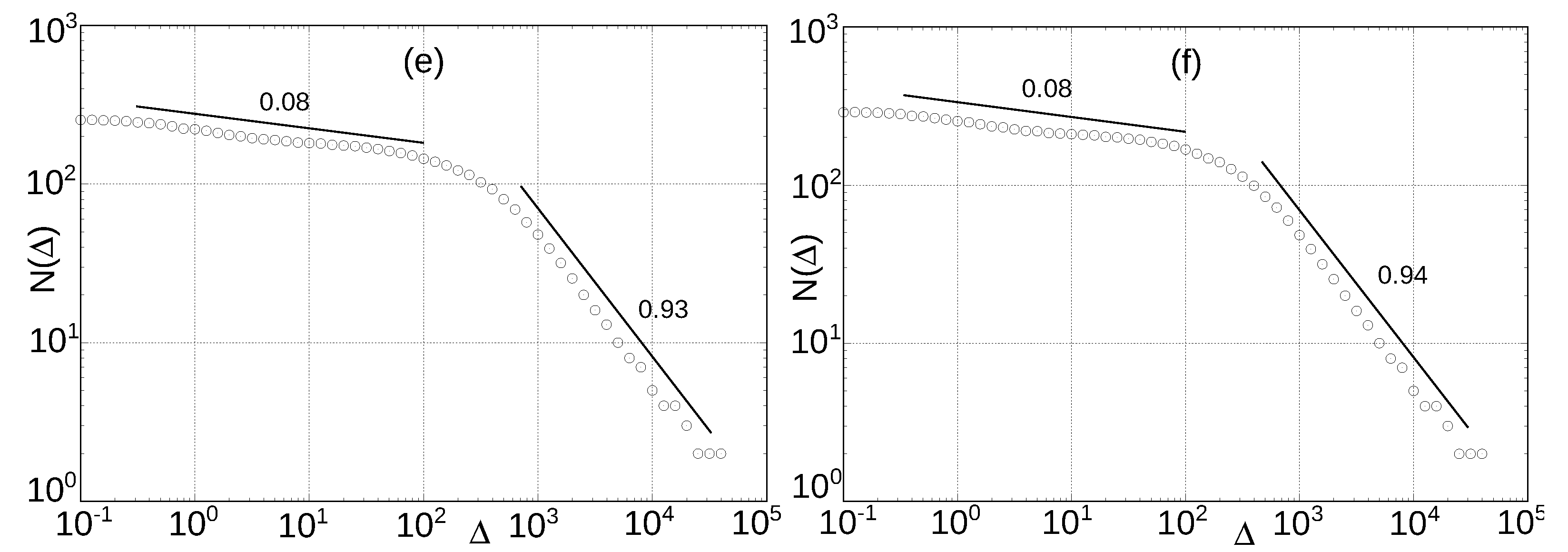
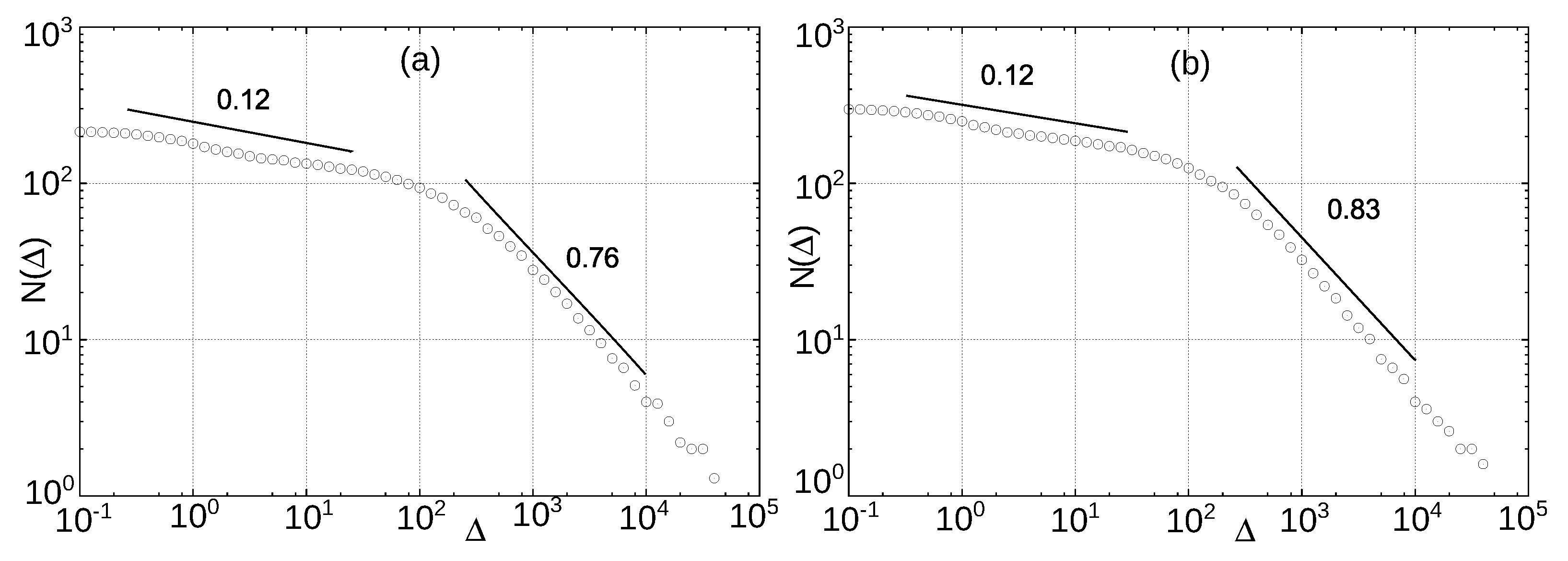
5.1. Hausdorff Dimension of the Polarity Timescale

Each trajectory of the phase variable y ( t ) in model (30) on the time interval 0 ; T can be considered as a possible variant of the geomagnetic field poloidal component evolution. Since we are considering a single-mode approximation for this component, we can only speak about the most general characteristics of the field, for example, about the direction of its polarity.
At the same time, it is polarity that is the most clearly defined characteristic of the behavior of a real field in the geological history of the Earth.
It is known that the GMPTS is a fractal set. The method for calculating the dimension of this scale was described in [34]. We will apply this method to our model polarity scale. The polarity value in the model determines the sign y ( t ) . The reversal into the model is the sign change.
The method for calculating the Hausdorff dimension of the scale is as follows.
On the scale of T length, some interval of length Δ is distinguished. N ( Δ ) is the number of intervals of length Δ on 0 ; T , on which at least one reversal occurs. There are two limiting cases. First case—if Δ T and the reversal are distributed approximately uniformly, then N ( Δ ) Δ 1 . In the second case Δ T and obviously N ( Δ ) Δ 0 .
Then, in a more general case, when Δ T and the reversals are not uniformly distributed, we can expect a dependence of the form:
N Δ = M · Δ d ,
where M is the Hausdorff measure and d is the Hausdorff dimension.
We made calculations in model (30) for the above fixed parameters and for various ν from 1.1 to 3.5 . The value of Δ changed with a uniform step in the log-scale from 10 1 to 4 · 10 5 .
To obtain stable statistical characteristics, we obtained 20 realizations of phase variable evolutions for each combination of parameters. The distributions N Δ and histograms of polarity intervals presented below are obtained by averaging over these realizations.
For values ν < 2 , non-zero values of the process ξ ( t ) (coherent structures) and reversals appeared very rarely. This did not allow obtaining stable estimates and the very number of reversals is improbably small. Sufficiently good statistical estimates were obtained for ν 2 . The resulting dependencies N ( Δ ) for some ν are shown in Figure 6 and Figure 7.
It is clearly seen that for all values of ν there are two straight segments on the graphs. The slope of each of the segments is signed in the figure. This slope corresponds to the value of d.
The slope for large values of Δ > 100 increases with ν , so it is controlled by the distribution of the waiting time τ W . Note that, according to the data of [34], Hausdorff dimensions for GMPTS for 170 Myr, 560 Myr, and 1700 Myr are 0.88, 0.83, and 0.87, respectively. It turns out that the real fractal dimension in the model polarity scale corresponds to the value ν = 2.3 .
The second straight section in the graphs of Figure 6 has a fixed slope, and a very small one at that. This second fractal dimension manifests itself in the region of small Δ . Most likely, this is due to the influence of the coherent structures lifetime τ E distribution, which was fixed in the calculations. The exponential distribution law corresponds to the Poisson process. It is known that a Poisson-type process, whose parameter has a trend, can have a fractal trajectory [11].
Note that for large values of Δ , there is no significant difference for models with energy suppression and helicity. The differences are very small and no regularity can be seen in them. However, for small Δ , α -quenching by energy gives a more fractal polarity scale. This is an interesting mathematical fact, but it is premature to talk about its physical meaning for an arbitrarily chosen K ( s ) and parameters.

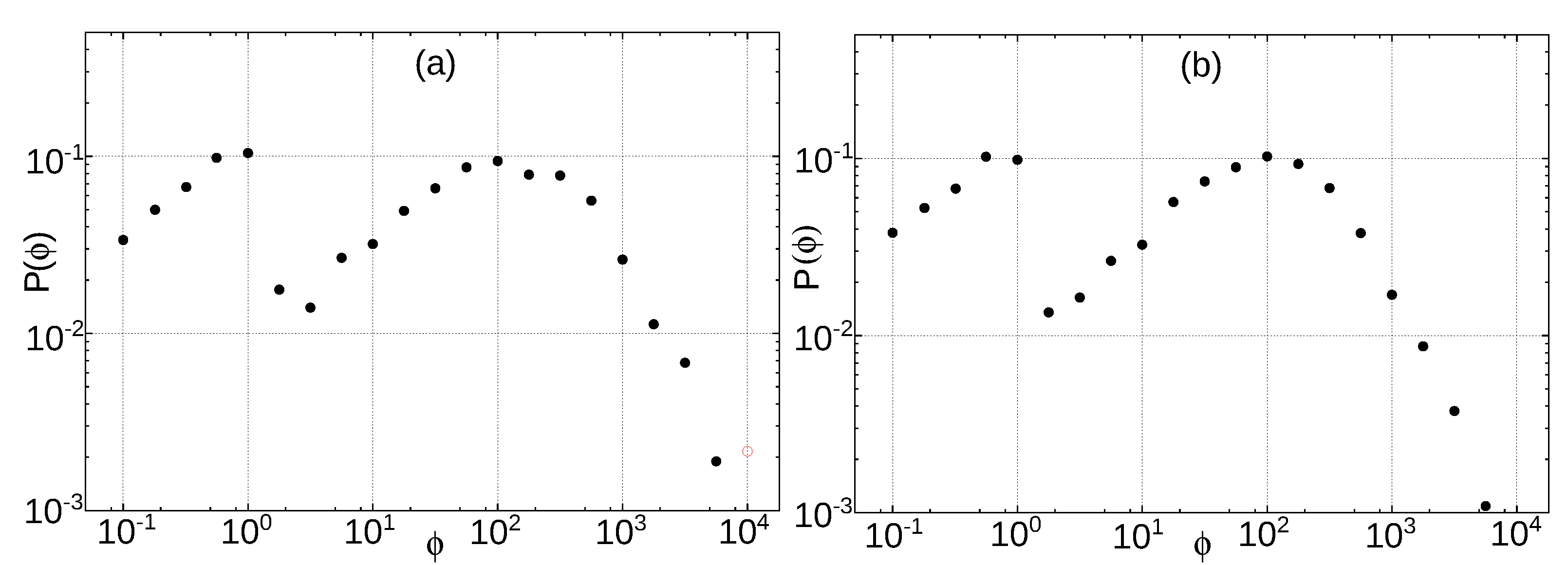
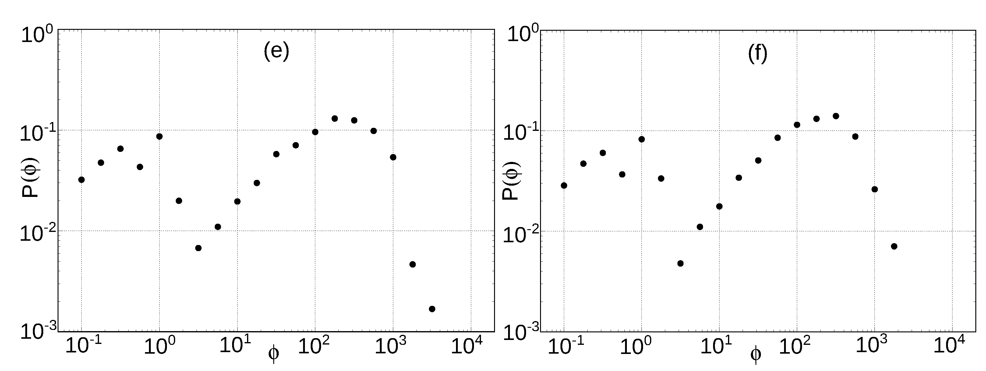
5.2. Distribution of the Polarity Intervals

The distributions of the polarity intervals lengths ϕ for model with α -quenching by helicity are shown in Figure 8 on a log-scale. The vertical axis is the probability P ( ϕ ) of occurrence of an length interval ϕ . The straight section starts approximately from the value ϕ = 300 . Compared to Figure 4, the power dependence is not so clear, so it is impossible to talk about differences in the slope of different ν . Approximately, this slope is 1.2 ÷ 1.9 . It grows with the growth of the ν .
It is also interesting to note that the histogram has a maximum at ν = 10 2 . This position of the maximum coincides with the point where the fractal dimensions of the polarity scale change. Apparently, the action of two different processes is also manifested here.
Histograms for the model with α -quenching by energy are shown in Figure 9. Here, the power-law tail of the distribution is not so clearly expressed, although it is also present. The distribution maximum is also shifted to the right by half an order.
So, the distribution of polarity intervals has a clearly defined power-law tail. The scatter of the observed values is five orders of magnitude. The presence of a clearly defined maximum and a power-law tail of the distribution of polarity intervals is also characteristic of the GMPTS.
We also note that there are no significant differences in the studied properties of the polarity scale for the two types of α -quenching.

6. Conclusions

Cosmic dynamo systems demonstrate very complex dynamic regimes, including regular and chaotic oscillations, periods of stabilization, excursions, and bursts. Therefore, it is not necessary to speak about the possibility of reproducing real magnetic fields evolution in models. We can only talk about the reproduction of some averaged statistical characteristics. To do this, it is necessary to have the possibility of a large set of long-term implementations of model evolutions. In addition, it is necessary to study the dependence on the control parameters. However, simulation of the time evolution of a dynamo system over time intervals of 10 9 years is possible only for low-mode approximations of the dynamo equations.
A feature of the geomagnetic polarity scale is the lack of a characteristic waiting time of reversal and self-similarity at different scales. The value intervals polarity covers several orders of magnitude and the polarity scale is chaotic [2,9,10,11,35]. One of the problems of the geodynamo theory is the explanation of this phenomenon and reproducing a series with similar statistical properties in numerical simulation. Some stochastic properties of a paleomagnetic scale were obtained by dynamical systems of low dimension [36,37,38,39].
In these works, models that do not have dynamic memory were studied. However, it is known that memory can have a strong influence on the operation of the dynamo [6].
The traditional way to introduce memory into dynamic models is to use integral operators. It has now become popular to use fractional calculus for memory modeling.
A fractional two-mode α ω -dynamo model is studied in this work. The Riemann–Liouville fractional differentiation operator is used to model the memory effect in the suppression of the α -effect by the helicity and energy of the magnetic field. The influence of discarded small-scale modes is modeled by a random process. The structure of this process imitates the spontaneous formation and destruction of coherent structures from small-scale modes.
For the numerical study of the model, a difference scheme has been especially developed, implemented in the C++ code. Verification of the code and scheme was performed on a particular case of a model with a priori known dynamics.
Multiple simulations of the time evolution of the model have been carried out. The Hausdorff dimension of the polarity scale of solutions is calculated. It turned out that for some values of the control parameters, a dimension is obtained that coincides with the dimension of real GMPTS. It is shown that the distribution of polarity intervals has a power-law tail and they cover several orders of magnitude. This also corresponds to real GMPTS.
In general, we can say that the described model reproduces the main features of GMPTS.
The numerical scheme makes it easy to adapt the model for various memory operators. Additionally, this model can be further modified for the α 2 - and α 2 ω -dynamo.

Author Contributions

Author Contributions: Conceptualization, G.V.; methodology, G.V.; software, L.F.; validation, L.F.; formal analysis, G.V. and L.F.; investigation, L.F.; resources, L.F. and G.V.; data curation, L.F.; writing—original draft preparation, L.F.; writing—review and editing, G.V.; visualization, L.F.; supervision, G.V.; project administration, G.V.; funding acquisition, G.V. All authors have read and agreed to the published version of the manuscript.

Funding

This research was funded by Russian Science Foundation grant number 22-11-00064 https://rscf.ru/project/22-11-00064/ (accessed on 9 June 2022).

Institutional Review Board Statement

Not applicable.

Informed Consent Statement

Not applicable.

Data Availability Statement

Not applicable.

Conflicts of Interest

The authors declare no conflict of interest.

Abbreviations

The following abbreviations are used in this manuscript:
GMPTSGeoMagnetic Polarity TimeScale

Appendix A. Expressions for the Difference Scheme Coefficients

The coefficients a i in Equation (27) are determined by substituting x n + 1 , q n + 1 and z n + 1 from (28) into the second Equation (23). This substitution and determination of coefficients requires complex transformations of algebraic expressions. Therefore, we carried out substitution and transformations using the computer algebra system Maple. As a result, the following formulas were obtained:
a 0 = A 01 y n + A 02 x n + 1 + V + A 03 x n ξ n z n + V ξ n + 1 L + A 04 V 3 , a 1 = A 11 ξ n + 1 L + A 12 V 2 + A 13 , a 2 = A 21 V , a 3 = h 2 6 K 0 W U ,
where
U = h μ 2 + h μ V = 2 x n + h μ y n x n 2 + h μ W = γ r U 2 + 1 r + ( 1 γ ) U A 01 = 1 h / 2 , A 02 = h D / 2 , A 03 = h / 2 , A 04 = h 2 K 0 γ r / 6 A 11 = h U / 2 , A 12 = h 2 K 0 ( 3 γ r U + 1 γ ) / 6 , A 13 = 1 + h ( D U 1 ) / 2 A 21 = h 2 K 0 [ ( 2 γ r U + 1 γ ) U + W ] / 6
It is clearly seen that the coefficients U , W , A i j , a 3 do not depend on time. Therefore, they must be calculated in the program once before the time loop. The coefficients V , a 0 , a 1 , a 2 change over time, so they need to be recalculated at each time step.

Appendix B. C++ Code for the Simulation

In this appendix, we present the main fragments of the C++ code with which the simulation was carried out.
First, macro definitions for constants 2 π and ln 2 :
#define PI2  6.283185307179586
#define log2  .6931471805599453
Next, the definition of functions for generating random values of the waiting time τ k W , the existing time τ k E and the process ξ k magnitude. The expressions (15) were used to generate τ k W and τ k E . The following expressions were used to generate the magnitude ξ k N ( 0 , σ 2 ) :
σ 2 ln U 1 cos 2 π U 2 ,
where random variables U 1 , U 2 are independent and uniform on 0 ; 1 .
double random_existing_time(double T_E) {
  double U=double(rand())/RAND_MAX;
  return -T_E/log2*log(U);
}
double random_waiting_time(double T_W,double nu, double c) {
  double U=double(rand())/RAND_MAX;
  return c*T_W*(pow(U,1./(1.-nu))-1.);
}
double random_xi(double sigma) {
  double U1=double(rand())/RAND_MAX;
  double U2=double(rand())/RAND_MAX;
  return sigma*sqrt(-2.*log(U1))*cos(PI2*U2);
}
The following function noise is needed to generate the values of the process ξ ( t ) at the points t n + 1 . For this, the value ξ ( t n ) , the boolean marker of the process state (the existence of a coherent structure) *p_coherence and the moment of the nearest switching between states *p_switch_time are used.
This function is called from the main program only if *p_switch_time lies between t n and t n + 1 . Otherwise, changing the value of ξ ( t ) is not required.
void noise(bool* p_coherence, double* p_switch_time, double* p_xi_next,
   double TW, double TE, double nu, double sigma, double dt) {
  double tau;
  double c=1./(pow(2.,1./(nu-1.))-1.);
  if (*p_coherence) {
    *p_xi_next=0.;
    do {tau=random_waiting_time(T_W,nu,c);} while (tau<dt+(1.e-10));
*p_switch_time+=tau;
  }
  else {
*p_xi_next=random_xi(sigma);
    do {tau=random_existing_time(T_E);} while (q<dt+(1.e-10));
*p_switch_time+=tau;
}
*p_coherence=!(*p_coherence);
return;
}
The following function calculates kernel values K n , n = 0 , 1 , , N by kernel type number, time step and kernel parameters p and ν (if last present). Possible types of kernels are indicated in the comments in the code. Note that the first type of kernel corresponds to the case of a fractional system.
double K_(int kernel_type,double s,double beta) {
  double result;
  double coef=1./tgamma(1.-beta);
  switch (ker_type) {
    case 1:  // K(s)=s^(-beta)/GAMMA(1-beta)
      result=pow(s,-beta)*coef;
      break;
    case 2:  // K(s)=1/(1+s)^beta
      result=pow(1.+s,-beta);
      break;
    case 3:  // K(s)=s/(1+s)^(1+beta)
      result=pow(1.+s,-1.-beta)*s;
      break;
    case 4:  // K(s)=s^beta*exp(-s);
      result=pow(s,beta)*exp(-s);
      break;
    default:  // K(s)=exp(-s)
      result=exp(-s);
      break;
  }
  return result;
}
The structure for the linked list q r , γ x ( t n ) , y ( t n ) values:
struct List {
  double Value;
  List *next;
};
The list of program input parameters and their meaning:
double D;        // relative dynamo number
double mu;       // inverse time of toroidal field decay
int kernel_type; // type of a quenching kernel: 1 - 5
double p;        // time scale of a kernel
double beta;     // exponent in the 1-4 kernels types
double gamma;    // parameter of the quadratic form q, eq. (7)
double r;        // ratio of toroidal and poloidal modes scales
double T_W;      // median of a coherent structure waiting time
double nu;       // exponent in the waiting time powe-law distribution
double sigma;    // process xi(t) standard deviation
double T_E;      // median of a coherent structure existing time
double T;        // time of simulation
double dt;       // time step
double BT;       // initial condition for toroidal field x(t)
double BP;       // initial condition for poloidal field y(t)
The main part of the program. This part, together with the declaration of input parameters and their initialization block, form the main() function.
srand(time(NULL));
double cutoff=T;
int N=int(floor(cutoff/dt)+1.);
if ((N&1)) N++;
double* K=new double[N+2];
double* Q=new double[N+1];
if (ker_type==1)
  K[0]=(1.+beta)*K_(kernel_type,0.1*dt/p,beta);
else
  K[0]=K_(kernel_type,0.,beta);
for(int i=1;i<=N+1;i++) K[i]=K_(kernel_type,i*dt/p,beta);
double U=dt*mu/(2.+dt*mu);
double W=gamma*(r*U*U+1./r)+(1.-gamma)*U;
double a3=-dt*dt/6.*K[0]*W*U; //OK
double A2=-dt*dt/6.*K[0]*((2.*gamma*r*U+1.-gamma)*U+W);
double A11=dt*U/2.;
double A12=-dt*dt*K[0]/6.*(3.*gamma*r*U+1.-gamma);
double A13=-1.+dt/2.*(D*U-1.);
double A01=1.-dt/2.;
double A02=dt*D/2.;
double A03=dt/2.;
double A04=-dt*dt*K[0]*gamma*r/6.;
double R1=2.+dt*mu;
double R2=dt*mu;
double R3=dt/3.*K[0];
double R4=dt/3.;
double R5=2.*dt/3.;
double a3_3=a3*3.;
double t=0.;
double z=0.;
bool coherence=false;
double c=1./(pow(2.,1./(nu-1.))-1.);
double switch_time=random_waiting_time(T_W,nu,c);
double xi=0.;
ofstream OutFile("result.txt");
ofstream OutReversals("reversals.txt");
OutFile.width(15); OutFile.precision(4); OutFile << fixed << t;
OutFile.width(15); OutFile.precision(6); OutFile << fixed << BT;
OutFile.width(15); OutFile.precision(6); OutFile << fixed << BP;
OutFile.width(15); OutFile.precision(6); OutFile << fixed << z;
OutFile.width(15); OutFile.precision(6); OutFile << fixed << xi;
OutFile << "\n";
double L,L1,L4,L2,xi_next,V,V2,V3,a2,a1,a0,newton_y,a2_2,newton_y2,
newton_y3,next_newton_y,newton_err,t_next;
int n=0; int k;
bool even=true;
Q[0]=gamma*(r*BT*BT+BP*BP/r)+(1.-gamma)*BT*BP;
while (n<N) {
  if (even==true) {
L1=L2=0.;
for(k=0;k<=n;k+=2) L1+=K[n+1-k]*Q[k];
for(k=1;k<=n-1;k+=2) L2+=K[n+1-k]*Q[k];
L=R5*(2.*L1+L2);
  }
  else {
  L1=L2=0.;
  for(k=1;k<=n;k+=2) L1+=K[n+1-k]*Q[k];
  for(k=2;k<=n-1;k+=2) L2+=K[n+1-k]*Q[k];
  L=R4*K[n+1]*Q[0]+R5*(2.*L1+L2);
  }
  t_next=t+dt;
  if ((t<switch_time)&&(t_next>=switch_time)) {
    noise(&coherence,&switch_time,&xi_next,TW,TE,nu,sigma,dt);
  }
  else xi_next=xi;
  V=(2.*BT+R2*(BP-BT))/R1;
  V2=V*V;
  V3=V2*V;
  a2=A2*V;
  a2_2=a2*2.;
  a1=A13+A11*(xi_next-L)+A12*V2;
  a0=A01*BP+A02*(BT+V)+A03*(BT*(xi-z)+V*(xi_next-L))+A04*V3;
  newton_y=BP;
  do {
    newton_y2=newton_y*newton_y;
    newton_y3=newton_y2*newton_y;
next_newton_y=newton_y-(a0+a1*newton_y+a2*newton_y2+a3*newton_y3)/
              (a1+a2_2*newton_y+a3_3*newton_y2);
newton_err=fabs(newton_y-next_newton_y);
  newton_y=next_newton_y;
  }
  while (newton_err>1e-10);
  if (((newton_y>0)&&(BP<0))||((newton_y<0)&&(BP>0)))
    OutReversals << t+dt/2. << "\n";
  BP=newton_y;
  BT=U*BP+V;
  Q[n+1]=gamma*(r*BT*BT+BP*BP/r)+(1.-gamma)*BT*BP;
  z=L+R3*Q[n+1];
  xi=xi_next;
  t=t_next;
  n++;
  even=!even;
  OutFile.width(15); OutFile.precision(4); OutFile << fixed << t;
  OutFile.width(15); OutFile.precision(6); OutFile << fixed << BT;
  OutFile.width(15); OutFile.precision(6); OutFile << fixed << BP;
  OutFile.width(15); OutFile.precision(6); OutFile << fixed << z;
  OutFile.width(15); OutFile.precision(6); OutFile << fixed << xi;
  OutFile << "\n";
}
List* pFirst;
pFirst=new List;
pFirst->Value=Q[0];
List* pLast;
pLast=pFirst;
List* ptmp;
for(int i=1;i<=N;i++) {
  ptmp=new List; pLast->next=ptmp;
  ptmp->Value=Q[i]; pLast=ptmp;
}
pLast->next=pFirst;
while (t<T) {
  L4=L2=0.;
  ptmp=pFirst;
  for(int i=N+1;i<=3;i-=2) {
    L4+=K[i]*ptmp->Value;
    ptmp=ptmp->next;
    L2+=K[i-1]*ptmp->Value;
    ptmp=ptmp->next;
  }
  L4+=K[1]*ptmp->Value;
  L=R5*(2.*L4+L2);
  t_next=t+dt;
  if ((t<switch_time)&&(t_next>=switch_time)) {
      noise(&coherence,&switch_time,&xi_next,TW,TE,nu,sigma,dt);
  }
  else xi_next=xi;
  V=(2.*BT+R2*(BP-BT))/R1;
  V2=V*V;
  V3=V2*V;
  a2=A2*V;
  a2_2=a2*2.;
  a1=A13+A11*(xi_next-L)+A12*V2;
  a0=A01*BP+A02*(BT+V)+A03*(BT*(xi-z)+V*(xi_next-L))+A04*V3;
  newton_y=BP;
  do {
    newton_y2=newton_y*newton_y;
    newton_y3=newton_y2*newton_y;
    next_newton_y=newton_y-(a0+a1*newton_y+a2*newton_y2+a3*newton_y3)/
                  (a1+a2_2*newton_y+a3_3*newton_y2);
    newton_err=fabs(newton_y-next_newton_y);
    newton_y=next_newton_y;
  }
  while (newton_err>1e-10);
  if (((newton_y>0)&&(BP<0))||((newton_y<0)&&(BP>0)))
    OutReversals << t+dt/2. << "\n";
  BP=newton_y;
  BT=U*BP+V;
  pFirst->Value=gamma*(r*BT*BT+BP*BP/r)+(1.-gamma)*BT*BP;
  z=L+R3*(pFirst->Value);
  pFirst=pFirst->next;
  pLast=pLast->next;
  xi=xi_next;
  t=t_next;
  n++;
  OutFile.width(15); OutFile.precision(4); OutFile << fixed << t;
  OutFile.width(15); OutFile.precision(6); OutFile << fixed << BT;
  OutFile.width(15); OutFile.precision(6); OutFile << fixed << BP;
  OutFile.width(15); OutFile.precision(6); OutFile << fixed << z;
  OutFile.width(15); OutFile.precision(6); OutFile << fixed << xi;
  OutFile << "\n";
}
OutFile.close();
OutReversals.close();
The program writes two files. The first "result.txt" contains columns of variables t, x ( t ) , y ( t ) , z ( t ) , ξ ( t ) . The second "reversals.txt" contains the moments of reversals.

References

  1. Zeldovich, Y.B.; Rusmaikin, A.A.; Sokoloff, D.D. Magnetic Fields in Astrophysics. The Fluid Mechanics of Astrophysics and Geophysics; Gordon and Breach: New York, NY, USA, 1983. [Google Scholar]
  2. Merril, R.T.; McElhinny, M.W.; McFadden, P.L. The Magnetic Field of the Earth: Paleomagnetism, the Core, and the Deep Mantle; Academic Press: London, UK, 1996. [Google Scholar]
  3. Stix, M. The Sun. An Introduction; Springer: Berlin/Heidelberg, Germany; New York, NY, USA, 1989. [Google Scholar]
  4. Parker, E.N. Hydromagnetic dynamo models. Astrophys. J. 1955, 122, 293–314. [Google Scholar] [CrossRef]
  5. Krause, F.; Rädler, K.-H. Mean-Filed Magnetohydrodynamics and Dynamo Theory; Academic-Verlag: Berlin, Germany, 1980. [Google Scholar]
  6. Hori, K.; Yoshida, S. Non-local memory effects of the electromotive force by fluid motion with helicity and two-dimensional periodicity. Geophys. Astrophys. Fluid Dyn. 2008, 102, 601–632. [Google Scholar] [CrossRef]
  7. Brandenburg, A. Memory effects in turbulent transport. Astrophys. J. 2009, 706, 712–726. [Google Scholar]
  8. Vodinchar, G. Hereditary Oscillator Associated with the Model of a Large-Scale αΩ-Dynamo. Mathematics 2020, 8, 2065. [Google Scholar] [CrossRef]
  9. Pechersky, D.M. Some characteristics of the geomagnetic field for 1700 Myears. Physica Zemli. 1997, 5, 3–20. (In Russian) [Google Scholar]
  10. Ermushev, A.V.; Rusmaikin, A.A.; Sokoloff, D.D. Fractal nature of the sequence of reverscals of the geomagnetic field. Magnetyhydrodynamics 1992, 4, 326–330. [Google Scholar]
  11. Gaffin, S. Analysis of scaling in the geomagnetic polarity reversal record. Phys. Earth Planet. Inter. 1989, 57, 284–290. [Google Scholar] [CrossRef]
  12. Anufriev, A.; Sokoloff, D. Fractal properties of geodynamo models. Geophys. Astrophys. Fluid Dyn. 1994, 74, 207–223. [Google Scholar] [CrossRef]
  13. Hollerbach, R.; Barenghi, C.; Lones, C. Taylor’s constraint in a spherical αω-dynamo. Geophys. Astrophys. Fluid Dyn. 1992, 67, 3–25. [Google Scholar] [CrossRef]
  14. Feschenko, L.; Vodinchar, G. Reversals in the large-scale αΩ-dynamo with memory. Nonlinear Process. Geophys. 2015, 22, 361–369. [Google Scholar] [CrossRef] [Green Version]
  15. Handbook of Fractional Calculus with Applications; Tenreiro, J.A.; De Gruyter, M. (Eds.) GmbH: Berlin, Germany; Boston, MA, USA, 2019. [Google Scholar]
  16. Herrmann, R. Fractional Calculus: An Introduction for Physicists; World Scientific: Singapore, 2014. [Google Scholar]
  17. Uchaikin, V. Fractional Derivatives Method; Artichoke: Ulyanovsk, Russia, 2008. (In Russian) [Google Scholar]
  18. Pope, S. Turbulent Flows; Cambridge University Press: Cambridge, UK, 2000. [Google Scholar]
  19. Field, G.B.; Blackman, E.G. Quenching of the α2 Dynamo. Astrophys. J. 2002, 572, 685–692. [Google Scholar] [CrossRef] [Green Version]
  20. Brandenburg, A.; Sandin, C. Catastrophic alpha quenching alleviated by helicity flux and shear. Astron. Astrophys. 2004, 427, 13–21. [Google Scholar] [CrossRef]
  21. Ruzmaikin, A. The Solar Cycle a a Strange Attractor. Comments Astrophys. 1981, 9, 85–96. [Google Scholar]
  22. Knobloch, E. Chaos in the segmented disc dynamo. Phys. Lett. A 1981, 82, 439–440. [Google Scholar] [CrossRef]
  23. Vodinchar, G.; Kazakov, E. The Lorenz system and its generalizations as dynamo models with memory. E3S Web Conf. 2018, 62, 02011. [Google Scholar] [CrossRef]
  24. Kleeorin, K.; Ruzmaikin, A. Dynamics of the average turbulent helicity in a magnetic field. Magnetohydrodynamics 1982, 18, 116–122. [Google Scholar]
  25. Brandenburg, A.; Haugen, N.E.L.; Käpylä, P.J.; Sandin, C. The problem of small and large scale fields in the solar dynamo. Astron. Nachr. 2004, 326, 174–185. [Google Scholar] [CrossRef] [Green Version]
  26. Sur, S.; Subramanian, K. Galactic dynamo action in presence of stochastic α and shear. Mon. Not. R. Astron. Soc. Lett. 2008, 392, 6–10. [Google Scholar] [CrossRef] [Green Version]
  27. Dekker, K.; Verwer J., G. Stability of Runge-Kutta Methods for Stiff Nonlinear Differential Equations; North-Holland: Amsterdam, The Netherlands; New York, NY, USA; Oxford, UK, 1984. [Google Scholar]
  28. Lorenz, E. Deterministic nonperiodic flow. J. Atm. Sci. 1963, 20, 130–141. [Google Scholar] [CrossRef] [Green Version]
  29. Sparrow, C. The Lorenz Equations: Bifurcations, Chaos, and Strange Attractors; Springer: Berlin/Heidelberg, Germany; New York, NY, USA, 1982. [Google Scholar]
  30. Pchelintsev, A.N. Numerical and Physical Modeling of the Dynamics of the Lorenz System. Numer. Anal. Appl. 2014, 7, 159–167. [Google Scholar] [CrossRef]
  31. Sokoloff, D.; Nefedov, S. A small-mode approximation in the stellar dynamo problem. Numer. Methods Program. 2007, 8, 142–149. [Google Scholar]
  32. Roberts, P.H. Kinematic dynamo models. Phil. Trans. R. Soc. A 1972, 272, 663–668. [Google Scholar]
  33. Reshetnyak, M. Simulation of Dynamo Processes in Geophysics. Ph.D. Thesis, G. A. Gamburtsev Institute of Physics of the Earth, Moscow, Rusia, 2003. [Google Scholar]
  34. Pechersky, D.M.; Reshetnyak, M.Y.; Sokoloff, D.D. Fractal analysis of the geomagnetic polarity time scale. Geomagn. Aeron. 1997, 37, 132–142. (In Russian) [Google Scholar]
  35. Ivanov, S.S. Self-similarity of the geomagnetic field reversal sequence. Geomagn. Aeron. 1993, 33, 181–186. (In Russian) [Google Scholar]
  36. Schmitt, D.; Ossendrijver, M.A.J.H.; Hoyng, P. Magnetic field reversals and secular variation in a bistable dynamo model. Phys. Earth Planet. Inter. 2001, 125, 119–124. [Google Scholar] [CrossRef]
  37. Pétrélis, F.; Fauve, S.; Dormy, E.; Valet, J.P. Simple Mechanism for Reversals of Earth’s Magnetic Field. Phys. Rev. Lett. 2009, 102, 144503. [Google Scholar] [CrossRef] [PubMed] [Green Version]
  38. Rikitake, T. Electromagnetism and the Earth’s Interior; Elsevier: Amsterdam, The Netherlands, 1965. [Google Scholar]
  39. Chossat, P.; Ambruster, D.; Oprea, I. A heteroclinic Model of Geodynamo Reversals and Excursions. In Dynamo and Dynamics, a Mathematical Challenge; Kluwer Academic: Dordrecht, The Netherlands, 2001. [Google Scholar]
Figure 1. Example of numerical study of zero equilibrium point stability: K ( s ) = s β / Γ ( 1 β ) , β = 0.9 , μ = 3.37 , p = r = γ = 1 , T W = T E = 5 , ν = 2 , σ = 1.5 .
Fractalfract 06 00328 g001
Figure 2. Result of verification (Lorenz’s case): μ = 10 , p = 3 / 8 , x ( 0 ) = 0 , y ( 0 ) = 10 2 , h = 10 2 . (a) D = 25 —asymptotically stationary regime; (b) D = 25 —chaotic regime; (c) D = 28 —chaotic attractor; (d) D = 210 —quasi-periodic regime.
Fractalfract 06 00328 g002
Figure 3. Result of simulation—Lorenz’s case with the influence of random structures: μ = 10 , p = 3 / 8 , T W = 5 , T E = 5 , ν = 2 , σ = 5 , x ( 0 ) = 0 , y ( 0 ) = 10 2 , h = 10 2 .
Fractalfract 06 00328 g003
Figure 4. Simulation results for model (30) without the influence of a random process. The α -quenching by helicity ( γ = 0). The parameter p values are shown on the legends. The parameter D and β values on panels: (a) D = 20 , β = 0.5 ; (b) D = 100 , β = 0.5 ; (c) D = 20 , β = 0.9 ; (d) D = 100 , β = 0.9 .
Fractalfract 06 00328 g004
Figure 5. Simulation results for model (30) without the influence of a random process. The α -quenching by energy ( γ = 1). The parameter p values are shown on the legends. The parameter D and β values on panels: (a) D = 20 , β = 0.5 ; (b) D = 100 , β = 0.5 ; (c) D = 20 , β = 0.9 ; (d) D = 100 , β = 0.9 .
Fractalfract 06 00328 g005
Figure 6. Number of N ( Δ ) intervals of Δ length, which contain at least one reversal. The α -quenching by helicity ( γ = 0). (a) ν = 2.0 ; (b) ν = 2.2 ; (c) ν = 2.3 ; (d) ν = 2.6 ; (e) ν = 2.8 ; (f) ν = 3.3 .
Fractalfract 06 00328 g006aFractalfract 06 00328 g006b
Figure 7. Number of N ( Δ ) intervals of Δ length, which contain at least one reversal. The α -quenching by energy ( γ = 1). (a) ν = 2.0 ; (b) ν = 2.2 ; (c) ν = 2.3 ; (d) ν = 2.6 ; (e) ν = 2.8 ; (f) ν = 3.3 .
Fractalfract 06 00328 g007aFractalfract 06 00328 g007b
Figure 8. Distributions of the polarity intervals. The α -quenching by helicity ( γ = 0 ). (a) ν = 2.0 ; (b) ν = 2.2 ; (c) ν = 2.3 ; (d) ν = 2.6 ; (e) ν = 2.8 ; (f) ν = 3.3 .
Fractalfract 06 00328 g008aFractalfract 06 00328 g008b
Figure 9. Distributions of the polarity intervals. The α -quenching by energy ( γ = 1 ). (a) ν = 2.0 ; (b) ν = 2.2 ; (c) ν = 2.3 ; (d) ν = 2.6 ; (e) ν = 2.8 ; (f) ν = 3.3 .
Fractalfract 06 00328 g009aFractalfract 06 00328 g009b
Publisher’s Note: MDPI stays neutral with regard to jurisdictional claims in published maps and institutional affiliations.

