Article

On the Finite-Time Boundedness and Finite-Time Stability of Caputo-Type Fractional Order Neural Networks with Time Delay and Uncertain Terms

1
Department of Applied Sciences, G L Bajaj Institute of Technology and Management, Greater Noida 201306, India
2
Department of Applied Sciences, Krishna Engineering College, Ghaziabad 201007, India
3
Department of Mathematics, Thiruvalluvar University, Vellore 632115, India
4
Department of Mathematics, University of Texas at San Antonio, San Antonio, TX 78249, USA
5
Department of Applied Sciences, Dronacharya Group of Institutions, Greater Noida 201306, India
*
Authors to whom correspondence should be addressed.
Fractal Fract. 2022, 6(7), 368; https://doi.org/10.3390/fractalfract6070368
Submission received: 3 June 2022 / Revised: 24 June 2022 / Accepted: 28 June 2022 / Published: 30 June 2022

Abstract

:
This study investigates the problem of finite-time boundedness of a class of neural networks of Caputo fractional order with time delay and uncertain terms. New sufficient conditions are established by constructing suitable Lyapunov functionals to ensure that the addressed fractional-order uncertain neural networks are finite-time stable. Criteria for finite-time boundedness of the considered fractional-order uncertain models are also achieved. The obtained results are based on a newly developed property of Caputo fractional derivatives, properties of Mittag–Leffler functions and Laplace transforms. In addition, examples are developed to manifest the usefulness of our theoretical results.

1. Introduction

Fractional calculus is a branch of mathematics that covers topics such as derivatives and integrals of noninteger order [1,2,3,4]. The recent discoveries in fractional calculus applications shows that, fractional-order systems have an essential role in modelling of numerous processes studies in diverse areas of science and engineering [5,6].
On the other hand, neural network models have the capability to solve significant issues in emergency domains such as financial market forecasting, optimization, information processing, parallel computing, associative memory, etc. [7,8,9,10,11].
Additionally, the study of the dynamic behavior of neural network models of fractional order has quickly attracted enormous interest as a research area. Numerous qualitative properties of such neural network models differ from the corresponding properties of the classical integer-order models. Fractional-order derivatives can provide a magnificent instrument for the description of memory and hereditary properties of various materials. Thus, their use increases the degree of freedom in the modelled processes and make the models more accurate than the integer-order ones [12,13,14,15,16]. These advantages constitute the fractional calculus as leading tool in the design of adequate artificial neural networks and it is also applied in biological neuronal networks. See, for example, some very recent publications [17,18], and the references therein.
It is established in the existing literature that time delays are commonly experienced in artificial and biological neural networks. It has been endowed that the presence of time delays often causes improper dynamical performances such as behavioral degradation, developmental oscillation, or instability of the model. Hence, the stability analysis of neural network models of integer order with time delays has received excess consideration and crucial stability conditions have been established [19,20,21].
Correspondingly, there are also interesting stability results proposed for fractional-order neural networks models [22,23,24,25]. In fact, such neural network systems are considered as very adequate models in different fields, such as diffusion waves, viscoelastic systems, electrical circuits, quantitative finance, mechanics, acoustics, electromagnetism, propagation, signal processing, system identification, colored noises, etc. [26,27,28,29,30]. Thus, the study of fractional-order neural networks is fundamental to both theory and applications and that is why, the stability analysis of fractional-order linear and nonlinear dynamical systems has attracted an expanding attention. For example, the fractional Lyapunov direct method and the Mittag–Leffler stability of fractional-order nonautonomous systems have been studied in [31]. In [32], Linear Matrix Inequalities (LMIs) stability conditions for fractional-order systems have been discussed. In [33], the asymptotic stability of nonlinear fractional differential system with Caputo derivative is studied. In [34], the problem of generalized Mittag–Leffler stability of multi-variables fractional-order nonlinear systems is investigated.
The definition of the finite-time stability was firstly proposed by Kamenkov in [35]. It is related to a fixed time-interval during which the state of a system starting within a specified bound does not exceed. For finite-time stable systems, it was demonstrated that they might have not only faster convergence, but also better robustness and disturbance rejection properties [36]. It is also known that finite-time stability and asymptotic stability are independent concepts, which neither imply nor exclude each other. Furthermore, the classical Lyapunov stability notion is mainly concerned with the asymptotic behavior of the states and rarely deals with the description of state bounds [37,38,39,40,41,42]. Moreover, in numerous applied problems, it is necessary to conserve the states within some bounds during a specific time interval (see, [43,44,45,46,47]). The finite-time stability is sometimes recommended than traditional stability approaches because most real neural networks only operate over finite-time intervals. Thus, some significant contributions have been given in finite-time stability of fractional-order systems (see for instance, [48,49,50,51] and references therein). Moreover, fractional-order finite-time stable neural networks have engaged a great level of research interest in the past decade. In [52], the finite-time stability of fractional-order Hopfield neural networks with time delays has been studied. Another paper, [53], explores the finite-time stability of fractional-order complex valued neural networks with time delay. In [54], finite-time stability criteria for fractional-order Cohen–Grossberg BAM neural networks with time delays are proposed. However, the topic of finite-time stability of fractional neural networks is still not completely investigated. In all the above-cited papers on finite-time stability behavior of delayed fractional neural network models, the effect of uncertain parameters is not investigated. In addition, the finite-time boundedness concept has not yet been introduced and finite-time boundedness criteria has not yet been proposed for fractional-order neural networks. This is the first motivation for designing the present research.
In practice, real systems typically give some uncertainties due to environmental noises, uncertain or slowly varying parameters, etc. Hence, the investigation of finite-time stability with parametric uncertainties for such systems is very important [55]. The systems with uncertain values of their parameters are often called uncertain systems. Note that, uncertain chaotic systems are studied in [56,57,58,59], including fractional-order models [60,61,62]. However, to the best of our knowledge, the problem of finite-time boundedness of fractional-order uncertain neural networks with time delay is not yet recognized in the existing literature.
Motivated by the above discussions, in this research we investigate the finite-time boundedness for fractional-order neural networks with time delays and uncertain parameters. The analysis of the proposed results is based on the fractional Lyapunov approach and fractional differentiation. The obtained criteria are in terms of LMIs which are very appropriate for numerical simulations.
The main novelty of the paper is in the following five points:
(1)
The finite-time boundedness and finite-time stability concepts are adopted to a continuous model of neural networks of fractional order with time delays and uncertain parameters;
(2)
New finite-time boundedness and finite-time stability results are established;
(3)
A new property of Caputo fractional derivatives, properties of Mittag–Leffler functions and Laplace transforms are applied;
(4)
By using the Lyapunov functional approach and inequality techniques the obtained results are represented in terms of LMIs;
(5)
Two examples are explored to expose the efficiency of the proposed finite-time stability and finite-time boundedness results.
The rest of the manuscript is organized according to the following plan. The fractional-order neural network problem under consideration is formulated in Section 2, where some preliminary results are also presented. The main finite-time boundedness and finite-time stability results are established in Section 3. Section 4 is devoted to numerical examples with which we demonstrate the proposed new results. The conclusion notes are stated in Section 5.
Notation: Throughout this investigation, N will denote the set of all positive integer numbers, R n stands for the n-dimensional Euclidean space, R n × m is the space of all n × m real matrices. For a matrix B and two symmetric matrices A and C, A B * C denotes the symmetric matrix, where the symmetry term is denoted by *. The values λ max ( Q ) and λ min ( Q ) will denote the maximum and minimum eigenvalue of a symmetric matrix Q, respectively. The superscript T represents the transpose of a matrix (or vector). The identity matrix of the compatible dimension will be denoted by I, diag{...} expresses the block-diagonal matrix and . is the Euclidean norm in R n .

2. Problem Formulation and Preliminary Results

We will investigate a class of fractional-order uncertain neural networks with time varying delays of the type
D α x ( t ) = C x ( t ) + ( A + A ) f ( x ( t ) ) + ( B + B ) f ( x ( t τ a ) ) + H w ( t ) + J u ( t ) ,
where x ( t ) = [ x 1 ( t ) , x 2 ( t ) , , x n ( t ) ] T R n is the state vector of the fractional-order uncertain neural network system, f ( x ( t ) ) = [ f 1 ( x 1 ( t ) ) , f 2 ( x 2 ( t ) ) , , f n ( x n ( t ) ) ] T R n denotes the neuron activation function, C = d i a g { c 1 , c 2 , , c n } is the self-connection weight, A , B , H , J represent the interconnection weight matrices, τ a is a time delay which is a positive constant, A , B are real-valued unknown matrices representing parameter uncertainties and are supposed to be in the form
[ A B ] = D F ( t ) [ E a E b ] ,
where D , E a , E b are known constant real-valued matrices with adequate dimensions, F ( t ) is an unknown time-varying matrix with bounded Lebegue measurable elements such that
F T ( t ) F ( t ) I .
We will consider the uncertain model (1) under the following initial condition:
x ( t ) = φ ( t ) , t [ τ a , 0 ] .
In the model (1) we consider the “uncertain” parameters A , B that may greatly affect the qualitative behaviour of the system. In fact, a real system always involves uncertainties due to some disturbances in system, inaccuracy in model parameter measurements or noises from external inputs. Hence, the analysis of models with uncertainties is essential for theory and applications.
Among the commonly used definitions for the general fractional differentiation and integration, such as Riemann–Liouville, Grünwald–Letnikov, Caputo, and Antagana–Baleanu derivatives, we will use the Caputo-type fractional derivative in our introduced model (1). The reason for this is the fact that it has the superiority of dealing accordingly with initial conditions on initial value problems that are in a format consistent with that in the integer-order cases which is observed in most physical processes [22].
The following assumption will be made on the activation function.
Assumption 1.
The neuron activation functions f is bounded and Lipschitz continuous on R n , that is, there exists L = d i a g { l 1 , l 2 , , l n } with l k > 0 , k = 1 , , n for which
| | f ( u ) f ( v ) | | | | L ( u v ) | |
for any u , v R n .
For the presentation of the main results we will need the next lemmas and definitions. Without loss of generality, for the applied fractional integral and derivatives we will consider that lower limits to be 0 throughout the paper.
Definition 1
([56]). For any time constant T, two constants c ¯ 1 > 0 , c ¯ 2 > 0 , and a symmetric matrix R > 0 , the fractional-order neural network model (1) with u ( t ) = 0 is said to be finite-time bounded with respect to ( c ¯ 1 , c ¯ 2 , T , R ) , if
sup s [ τ a , 0 ] x T ( s ) R x ( s ) c ¯ 1 x T ( t ) R x ( t ) c ¯ 2 , t [ 0 , T ] .
Definition 2
([56]). For any time constant T, two constants c ¯ 1 > 0 , c ¯ 2 > 0 , and a symmetric matrix R > 0 , the fractional-order neural network system (1) with w ( t ) = 0 and u ( t ) = 0 is said to be finite-time stable with respect to ( c ¯ 1 , c ¯ 2 , T , R ) , if
sup s [ τ a , 0 ] x T ( s ) R x ( s ) c ¯ 1 x T ( t ) R x ( t ) c ¯ 2 , t [ 0 , T ] .
Definition 3
([59]). For any time constant T, the fractional-order neural network (1) is robustly finite-time stabilizable with a disturbance attenuation level β, if the corresponding fractional closed-loop neural network system with a controller u ( t ) = K x ( t ) , t ( 0 , T ] , is finite-time bounded.
Definition 4
([1]). The fractional integral of a noninteger order α for an integrable function x ( t ) , x ( t ) R n , is defined as
0 I t α x ( t ) = 1 Γ ( α ) 0 t ( t τ a ) α 1 x ( τ a ) d τ a ,
where Γ ( · ) is the Gamma function given by Γ = 0 θ t s 1 e t d t .
Definition 5
([1]). The fractional derivative of Caputo type of order α for a function x ( t ) is defined as
0 D t α x ( t ) = 1 Γ ( k α ) 0 t ( t τ a ) k α 1 x ( k ) ( τ a ) d τ a ,
where k 1 < α < k , k N .
Throughout the paper the fractional integral 0 I t α will be denoted by I α and the Caputo fractional derivative 0 D t α by D α for simplicity.
Lemma 1
([63]). For α ( 0 , 1 ) and continuous and differentiable on [ 0 , ] vector-function x ( t ) R n , we have
1 2 D α [ x T ( t ) x ( t ) ] x T ( t ) D α x ( t ) , t 0 .
Lemma 2
([64]). For α ( 0 , 1 ) , continuous and differentiable on [ 0 , ] vector-function x ( t ) R n and P > 0 , P R n × n , we have inequality
1 2 D α [ x T ( t ) P x ( t ) ] x T ( t ) P D α x ( t ) , t 0 .
Lemma 3
([1]). For k N and k 1 < α < k , the following relation is valid
I α ( D α x ( t ) ) = x ( t ) i = 0 k 1 x i ( 0 ) i ! t i .
In the case when 0 < α < 1 ,
I α ( D α x ( t ) ) = x ( t ) x ( 0 ) .
Lemma 4
([65]). Let x ( t ) and a ( t ) be non-negative and local integrable on [ 0 , T ] functions, T + . Assume that α > 0 , g ( t ) is a non-decreasing, nonnegative and continuous function defined on 0 t < T , g ( t ) M (constant), satisfying
x ( t ) a ( t ) + g ( t ) 0 t ( t s ) α 1 x ( s ) d s , t [ 0 , T ] .
If a ( t ) is non-decreasing on [ 0 , T ] , then
x ( t ) a ( t ) G α ( g ( t ) Γ ( α ) t α ) , t [ 0 , T ] ,
where G α is the Mittag–Leffler function.
Lemma 5
([58]). Assume that U , V , W and X be real matrices of adequate dimensions and X = X T . Then,
V T V I , X + U V W + U T V T W T < 0 ,
if and only if there exists a scalar δ > 0 such that X + δ U U T + δ 1 W T W < 0 .
Lemma 6
([19]). (Schur complement). For any constant matrices X , Y , Z , with X = X T and 0 < Y = Y T , we have X + Z T Y 1 Z < 0 , if and only if,
X Z T * Y < 0 o r Y Z * X < 0 .

3. Finite-Time Stability and Boundedness Results

3.1. Robust Finite-Time Stability

In this section we investigate the finite-time stability of uncertain fractional-order neural networks with time delays of the type
D α x ( t ) = C x ( t ) + ( A + A ) f ( x ( t ) ) + ( B + B ) f ( x ( t τ a ) ) ,
where the system parameters are as in (1).
Theorem 1.
For given scalars τ a , c ¯ 1 , c ¯ 2 , T and a symmetric matrix R > 0 the fractional-order neural network model (7) is finite-time stable with respect to ( c ¯ 1 , c ¯ 2 , T , R ) if there exist scalars δ 1 , δ 2 , δ 3 , β and a matrix P > 0 satisfying:
Θ ^ 1 = Θ 1 P D L T E a T δ 1 P D L T E b T δ 2 * δ 1 I 0 0 0 * * δ 1 I 0 0 * * * 2 δ 2 I 0 * * * * 2 δ 2 I < 0 ,
Θ ^ 2 = Θ 2 P D L T E b T δ 3 * 2 δ 3 I 0 * * 2 δ 3 I < 0 ,
G α ( β T α ) c o n d ( P ¯ ) < c ¯ 2 c ¯ 1 ,
where
Θ 1 = P C C T P T + P A L + L T A T P T + 1 2 P B L + 1 2 L T B T P T β P , Θ 2 = 1 2 P B L + 1 2 L T B T P T , P = R 1 / 2 P ¯ R 1 / 2 .
Proof. 
Consider the following Lyapunov functional:
V ( t ) = 1 2 x T ( t ) P x ( t ) .
For the fractional-order derivative of V ( x ( t ) ) along the system (7), by Lemma 2, we have
D α V ( t ) = 1 2 D α x T ( t ) P x ( t ) x T ( t ) P D α x ( t ) .
Hence,
D α V ( t ) x T ( t ) P [ C x ( t ) + ( A + D F ( t ) E a ) f ( x ( t ) ) + ( B + D F ( t ) E b ) f ( t τ a ) ] , = x T ( t ) P [ C + A L + D F ( t ) E a L ] x ( t ) + x T ( t ) P [ B L + D F ( t ) E b L ] x ( t τ a ) , = x T ( t ) P [ C + A L + D F ( t ) E a L + 1 2 B L + 1 2 D F ( t ) E b L ] x ( t ) + x T ( t τ a ) P [ 1 2 B L + 1 2 D F ( t ) E b L ] x ( t τ a ) , 1 2 x T ( t ) [ P C C T P T + P A L + L T A T P T + P D F ( t ) E a L + L T E a T F T ( t ) D T P T + 1 2 P B L + 1 2 L T B T P T + 1 2 P D F ( t ) E b L + 1 2 L T E b T F T ( t ) D T P T ] x ( t ) + x T ( t τ a ) [ 1 2 P B L + 1 2 L T B T P T + 1 2 P D F ( t ) E b L + 1 2 L T E b T F T ( t ) D T P T ] x ( t τ a ) .
Let the following inequalities be satisfied
Θ ^ 1 = P C C T P T + P A L + L T A T P T + P D F ( t ) E a L + L T E a T F T ( t ) D T P T + 1 2 P B L + 1 2 L T B T P T + 1 2 P D F ( t ) E b L + 1 2 L T E b T F T ( t ) D T P T < 0 ,
Θ ^ 2 = 1 2 P B L + 1 2 L T B T P T + 1 2 P D F ( t ) E b L + 1 2 L T E b T F T ( t ) D T P T < 0 .
By employing Lemma 11, the above inequalities can be written as
Θ ^ 1 = Θ 1 + δ 1 1 P D D T P T + δ 1 L T E a T E a L + 1 2 δ 2 1 P D D T P T + 1 2 δ 2 L T E b T E b L < 0 ,
Θ ^ 2 = Θ 2 + 1 2 δ 3 1 P D D T P T + 1 2 δ 3 L T E b T E b L < 0 .
By using Lemma 6, the inequalities (15) and (16) are equivalent, correspondingly, to the following LMIs:
Θ 1 P D L T E a T P D L T E b * δ 1 I 0 0 0 * * δ 1 1 * * * * * 2 δ 2 * * * * * 2 δ 2 1 < 0 ,
Θ 2 P D L T E b * 2 δ 3 0 * * 2 δ 3 1 < 0 .
After the pre- and post- multiplying of (17) by d i a g { I , I , δ 1 , I , δ 2 } and pre- and post-multiplying of (18) by d i a g { I , I , δ 3 } we obtain (8) and (9), respectively. On other hand, it is easy to check that inequalities (8), (9) imply the existence of a required constant β > 0 , such that
D α V ( x ( t ) ) < β sup s [ τ a , 0 ] V ( x ( s ) ) , t [ 0 , T ] .
The inequality (19) implies the existence of a nonnegative function M ( t ) satisfying
D α V ( x ( t ) ) + M ( t ) < β V ( x ( t ) ) , t [ 0 , T ] .
We apply the Laplace transform to (20) to obtain
s α V ( x ( s ) ) V ( x ( 0 ) ) s α 1 + M ( s ) = β V ( x ( s ) )
or, equivalently
V ( x ( s ) ) = ( s α β ) 1 V ( x ( 0 ) ) s α 1 M ( s ) .
Applying the inverse Laplace transform of (22), we obtain
V ( x ( t ) ) = V ( x ( 0 ) ) G α ( β t α ) 0 t M ( τ a ) [ ( t τ a ) α 1 G α , α ( β ( t τ a ) α ) ] d τ a .
Since both ( t τ a ) α 1 and G α , α ( β ( t τ a ) α ) are nonnegative functions, we obtain that,
V ( x ( t ) ) G α ( β t α ) V ( x ( 0 ) ) G α ( β t α ) sup s [ τ a , 0 ] V ( x ( s ) ) , t [ 0 , T ] .
Inequality (24) is equivalent to x T ( t ) P x ( t ) G α ( β t α ) sup s [ τ a , 0 ] x T ( s ) P x ( s ) noting that P = R 1 / 2 P ¯ R 1 / 2 which can be rewritten as
x T ( t ) R 1 / 2 P ¯ R 1 / 2 x ( t ) < G α ( β t α ) sup s [ τ a , 0 ] x T ( s ) R 1 / 2 P ¯ R 1 / 2 x ( s ) .
The above implies,
λ min ( P ¯ ) x T ( t ) R x ( t ) < λ max ( P ¯ ) G α ( β t α ) sup s [ τ a , 0 ] x T ( s ) R x ( s ) .
After considering sup s [ τ a , 0 ] x T ( s ) R x ( s ) c ¯ 1 together with (10), we have that x T ( t ) R x ( t ) < c ¯ 2 for t [ 0 , T ] , which completes the proof. □
Remark 1.
Theorem 1 offers criteria for finite-time stability of a class of delayed fractional-order neural networks under uncertainties. It contributes to the development of the finite-time stability theory of fractional neural network models and extend the existing results on the topic [48,49,50,51,52,53,54] to the uncertain case. Indeed, the presence of uncertain terms may lead to instability of a model even if the uncertainties are very small. In Table 1, a comparison table with previously published results is shown below.
Remark 2.
One of the most investigated stability behavior of neural networks models is the asymptotic stability and its special case of exponential stability [22,25,29,33]. For fractional-order systems the concept of exponential stability has been generalized to that of Mittag–Leffler stability [15,18,23,24,31]. Different from the existing results on asymptotic and Mittag–Leffler stability strategies of fractional-order systems we investigated the finite-time stability behavior of a delayed neural network system under uncertainties.

3.2. Finite-Time Boundedness

In this Section, we first provide a criterion for the finite-time boundedness of the delayed fractional-order neural network model of the type:
D α x ( t ) = C x ( t ) + ( A + A ) f ( x ( t ) ) + ( B + B ) f ( x ( t τ a ) ) + H w ( t ) .
Theorem 2.
For given scalars τ a , c ¯ 1 , c ¯ 2 , d, T and a symmetric matrix R > 0 the fractional-order neural network model with time delay (27) is finite-time bounded with respect to ( c ¯ 1 , c ¯ 2 , T , R , d ) , if there exist constants δ 1 , δ 2 , δ 3 , β and a matrix P ¯ > 0 such that the following LMIs:
Ψ ^ 1 = Ψ 1 P H P D L T E a T δ 1 P D L T E b T δ 2 * β I 0 0 0 0 * δ 1 I 0 0 0 * * δ 1 I 0 0 * * * 2 δ 2 I 0 * * * * 2 δ 2 I < 0 ,
Θ ^ 2 = Θ 2 P D L T E b T δ 3 * 2 δ 3 I 0 * * 2 δ 3 I < 0 ,
G α ( β T α ) β d T α Γ ( α + 1 ) + λ max ( P ¯ ) c ¯ 1 < λ min ( P ¯ ) c ¯ 2 ,
are satisfied, where
Ψ 1 = P C C T P T + P A L + L T A T P T + 1 2 P B L + 1 2 L T B T P T β P , Θ 2 = 1 2 P B L + 1 2 L T B T P T , P = R 1 / 2 P ¯ R 1 / 2 .
Proof. 
For the α th Caputo derivative of the Lyapunov functional (11), we get
D α V ( x ( t ) ) + β V ( x ( t ) ) + β w T ( t ) w ( t ) = ξ T ( t ) Ψ ^ 1 ξ ( t ) .
From (15) and (16) we obtain
Ψ ^ 1 = ξ T ( t ) Ψ 1 + δ 1 1 P D D T P T + δ 1 L T E a T E a L + 1 2 δ 2 1 P D D T P T + 1 2 δ 2 L T E b T E b L P H * β I ξ T ( t ) ,
Θ ^ 2 = Θ 2 + 1 2 δ 3 1 P D D T P T + 1 2 δ 3 L T E b T E b L ,
where ξ T ( t ) = [ x T ( t ) w T ( t ) ] . By applying Schur complement Lemma 6, we can obtain
Ψ 1 P H P D L T E a T P D L T E b * β I 0 0 0 0 * * δ 1 I 0 0 0 * * * δ 1 1 0 0 * * * * 2 δ 2 0 * * * * * 2 δ 2 1 < 0 ,
Θ 2 P D L T E b * 2 δ 3 0 * * 2 δ 3 1 < 0 .
Then by multiplying of both sides of (34) by d i a g { I , I , I , δ 1 , I , δ 2 } and multiplying of both sides of (35) by d i a g { I , I , δ 3 } , we get (28) and (29). This, together with w T ( t ) w ( t ) d gives
D α V ( x ( t ) ) < β V ( x ( t ) ) + β d , t [ 0 , T ] .
After an integration of order α of both sides of (36) from 0 to t T and applying Lemma 3, we obtain
V ( x ( t ) ) < sup s [ τ a , 0 ] V ( x ( s ) ) + β d t α Γ ( α + 1 ) + β Γ ( α ) 0 t ( t τ a ) α 1 V ( x ( τ a ) ) d τ a .
Now we apply Lemma 4 to obtain
V ( x ( t ) ) < sup s [ τ a , 0 ] V ( x ( s ) ) + β d t α Γ ( α + 1 ) G α ( β T α ) .
Noting that for P = R 1 / 2 P ¯ R 1 / 2 , the next relations are satisfied:
V ( x ( t ) ) = x T ( t ) P x ( t ) = x T ( t ) R 1 / 2 P ¯ R 1 / 2 x ( t ) λ min ( P ¯ ) x T ( t ) R x ( t ) ,
sup s [ τ a , 0 ] V ( x ( s ) ) = sup s [ τ a , 0 ] x T ( s ) R 1 / 2 P ¯ R 1 / 2 x ( s ) < λ max ( P ¯ ) sup s [ τ a , 0 ] x T ( s ) R x ( s ) λ max ( P ¯ ) c 1 .
From (38), it follows that
λ min ( P ¯ ) x T ( t ) R x ( t ) < G α ( β T α ) β d T α Γ ( α + 1 ) + λ max ( P ¯ ) c ¯ 1 .
By combining (41) and (30) we obtain
x T ( t ) R x ( t ) < c ¯ 2 , t [ 0 , T ] .
This completes the proof. □
Next, we consider the delayed fractional-order neural network system with uncertain terms and the state feedback controller u ( t ) = K x ( t ) as follows:
D α x ( t ) = C x ( t ) + ( A + A ) f ( x ( t ) ) + ( B + B ) f ( x ( t τ a ) ) + H w ( t ) + J u ( t ) ,
u ( t ) = K x ( t ) ,
where K is a scalar gain matrix.
Theorem 3.
For given scalars τ a , c ¯ 1 , c ¯ 2 , d, T and a symmetric matrix R > 0 the delayed fractional-order neural network model (43) is finite-time bounded with respect to ( c ¯ 1 , c ¯ 2 , T , R , d ) , if there exist scalars δ 1 > 0 , δ 2 > 0 , δ 3 > 0 , β > 0 and a matrix P ¯ > 0 which satisfy the following LMIs:
Φ ^ 1 = Φ ¯ 1 P H P D L T E a T δ 1 P D L T E b T δ 2 * β I 0 0 0 0 * δ 1 I 0 0 0 * * δ 1 I 0 0 * * * 2 δ 2 I 0 * * * * 2 δ 2 I < 0 ,
Θ ^ 2 = Θ 2 P D L T E b T δ 3 * 2 δ 3 I 0 * * 2 δ 3 I < 0 ,
G α ( β T α ) β d T α Γ ( α + 1 ) + λ max ( P ¯ ) c ¯ 1 < λ min ( P ¯ ) c ¯ 2 ,
where
Φ ¯ 1 = C P + J L P C T + L T J T + P A L + L T A T P T + 1 2 P B L + 1 2 L T B T P T β P , P = R 1 / 2 P ¯ R 1 / 2
and the gain matrix K = L P 1 .
Proof. 
By replacing C in the LMI (28) with C + L P 1 from the Theorem 1 we can obtain
Φ 1 P H P D L T E a T δ 1 P D L T E b T δ 2 * β I 0 0 0 0 * δ 1 I 0 0 0 * * δ 1 I 0 0 * * * 2 δ 2 I 0 * * * * 2 δ 2 I < 0 ,
Θ 2 P D L T E b T δ 3 * 2 δ 3 I 0 * * 2 δ 3 I < 0 ,
where
Φ 1 = ( C P J L P 1 ) P ( C J L P 1 ) T + P A L + L T A T P T + 1 2 P B L + 1 2 L T B T P T β P , Θ 2 = 1 2 P B L + 1 2 L T B T P T .
Hence, we have that the neural network system (43), which is considered as a closed-loop system, with the controller (44) is finite-time bounded with respect to ( c ¯ 1 , c ¯ 2 , T , R , d ) . The proof is completed. □
Remark 3.
Theorems 2 and 3 provide sufficient conditions for finite-time boundedness of fractional delayed neural network models. To the best of the authors’ knowledge such results are not offered for fractional-order models. With there results we extend the existing results on finite-time boundedness of integer-order systems [43,44,47] to the fractional-order models. In addition, uncertain terms are considered in the proposed fractional model.
Remark 4.
Theorem 3 also implies that system (43) is robustly finite-time stabilizable with respect to ( c ¯ 1 , c ¯ 2 , T , R , d ) according to Definition 1.

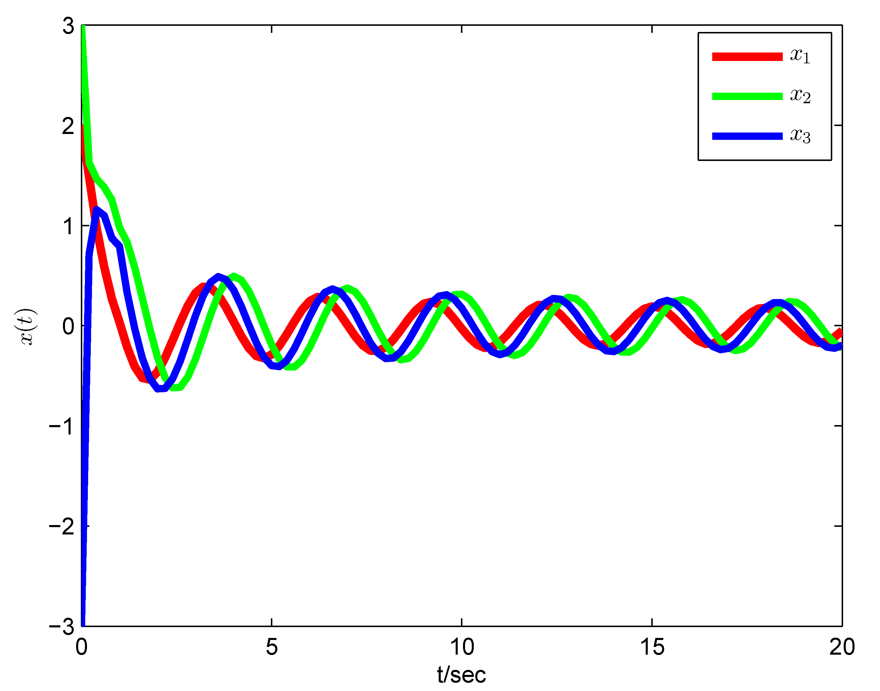
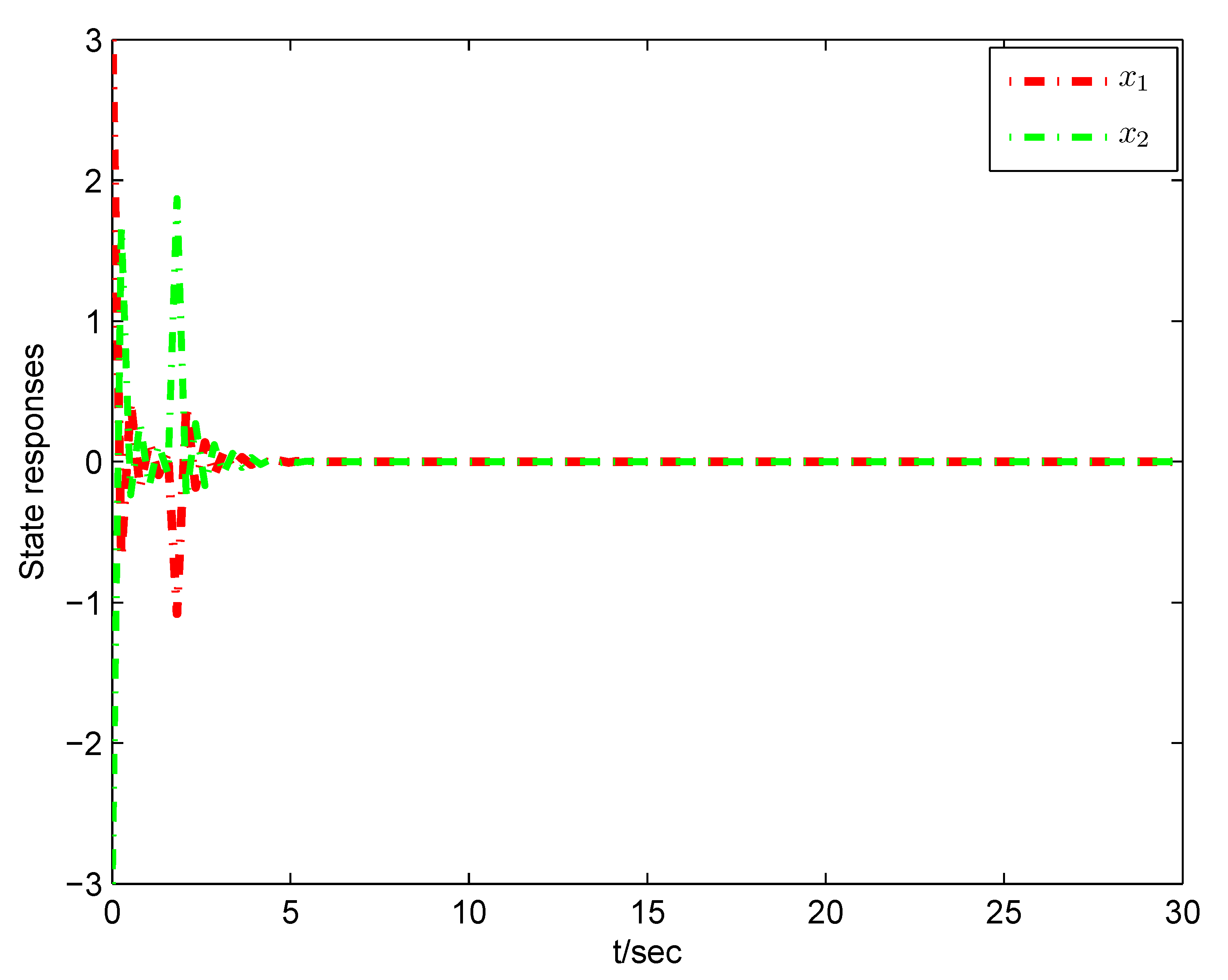
4. Numerical Examples

In this Section, numerical examples are addressed to demonstrate the usefulness of the proposed method.
Example 1.
Let us consider the fractional-order neural network system with a disturbance and uncertain terms defined by
D α x ( t ) = C x ( t ) + ( A + A ) f ( x ( t ) ) + ( B + B ) f ( x ( t τ a ) ) + H w ( t ) ,
with the following parameters:
C = 1 0 0 0 2 0 0 0 3 , A = 2 1.2 0.5 1.8 1.71 1.15 4.75 0.5 1.1 , B = 0.4 0.6 0.002 0.4 0.38 0.3 0.6 0.1 0.4 , H = 0.2 0.5 1.2 1.03 0.61 1.8 0.4 0.03 0.21 , E a = d i a g { 0.1 , 0.1 , 0.1 } , E b = d i a g { 0.1 , 0.1 , 0.1 } , L = d i a g { 1 , 1 , 1 } , α = 0.5 , τ a = 0.1 , d = 1 , β = 0.05 , c ¯ 1 = 2 , c ¯ 2 = 16 , R = I , T = 20 .
By solving (28)–(30) we obtain the achievable solutions as follows:
P ¯ = 0.0186 0.0032 0.0059 0.0032 0.0029 0.0011 0.0059 0.0011 0.0258 , δ 1 = 0.0874 , δ 2 = 0.2178 , δ 3 = 0.7989 .
Furthermore, Figure 1 represents the state responses of the fractional-order neural network model (50) with initial data at [ 3 , 3 ] T . It can be observed that the state trajectories of the fractional-order neural network system (50) with a disturbance and uncertain terms in Example 1 are bounded and thus the system is finite-time bounded with respect to ( c ¯ 1 , c ¯ 2 , T , R , d ) under the proposed conditions.
Remark 5.
In Example 1, a fractional-order neural network system with a disturbance and uncertain terms is considered and investigated using Theorem 2. The feasible solutions are obtained and it is demonstrated that they are finite-time bounded with respect to ( c ¯ 1 , c ¯ 2 , T , R , d ) . This shows that the proposed conditions of Theorem 2 are efficient and can be easily applied to check the finite-time boundedness behavior of the solutions of the fractional order neural networks. In addition, it can be seen by Figure 1 that the state trajectories converge in a finite time; hence, the system is also finite-time stable.
Example 2.
Consider the following fractional-order uncertain neural network
D α x ( t ) = C x ( t ) + ( A + A ) f ( x ( t ) ) + ( B + B ) f ( x ( t τ a ) ) + H w ( t ) + J u ( t ) ,
with
C = 2 0 0 3 , A = 4 3 9 5 , B = 2 0.5 0.5 2 , H = 0.2 0.1 0 0.2 , J = 0.3 0.5 0.5 0.2 , E a = d i a g { 0.2 , 0.2 } , E b = d i a g { 0.2 , 0.2 } , L = d i a g { 1 , 1 } , d = 1.2 , β = 0.3 , R = 2 I .
The system parameters are specified as follows: w ( t ) = s i n ( t ) , c ¯ 1 = 5 , c ¯ 2 = 7 , τ a = 0.5 . By solving the LMIs (45)–(47) in Theorem 3, we obtain the feasible solutions as
P ¯ = 0.6650 0.0205 0.0205 0.6894 , δ 1 = 2.0330 , δ 2 = 1.1690 , δ 3 = 1.1836 ,
and
K = 3.0102 0.0896 0.0896 2.9038 .
The state trajectories of system (51) are illustrated in Figure 2. It shows the state trajectories of the fractional order neural network model (51) are bounded in a very short time T = 5 s under the feedback control K; thus, the system is finite-time bounded with respect to ( c ¯ 1 , c ¯ 2 , T , R , d ) the proposed conditions. According to Definition 1, the model (51) is robustly finite-time stabilizable with respect to ( c ¯ 1 , c ¯ 2 , T , R , d ) .
Remark 6.
The efficiency of the conditions of Theorem 3 are demonstrated in Example 2. The feasible solutions and feedback control gain matrix K of a fractional-order neural network system with a disturbance and uncertain terms are obtained. The finite-time boundedness is demonstrated by solving the LMIs type conditions. In addition, the considered fractional order neural network model is robustly finite-time stabilizable with respect to ( c ¯ 1 , c ¯ 2 , T , R , d ) .

5. Conclusions

In this study, we considered the problem of finite-time boundedness of a class of fractional-order neural networks with time delays and uncertain terms. Based on the fractional differentiation and Lyapunov functional theory, we derived conditions that ensure the finite-time boundedness and finite-time stability under uncertainties. The presented criteria are in terms of LMIs, which are very suitable for numerical simulations. Finally, numerical examples are elaborated to manifest the efficacy and usefulness of our theoretical results. Our results contribute to the development of the finite-time stability theory of fractional-order neural network models. The presented finite-time boundedness results mark the beginning of their investigations for the proposed models. Since fractional-order neural networks have significant applications in diverse areas of science and engineering the derived criteria can be of interest to numerous pure and applied researchers. Moreover, the proposed finite-time boundedness results offer an important mechanism that is of importance in the study of periodic neural network models. It is possible to extend the results to the synchronization problem of complex-valued neural networks of fractional order with both leakage and discrete delays and stability of stochastic fractional-order neural networks. The future research scope of our investigations is also related to the effects continuous and impulsive controllers on the finite-time stability and finite-time boundedness behavior of the introduced model. In this cases, the presented finite-time stability criteria can be applied in the study of the finite-time robustness controllability of uncertain systems. The sensitivity analysis is another direction for the future research on the topic.

Author Contributions

Conceptualization, B.P., G.K.T., M.S.A., G.S., I.S. and P.K.S.; methodology, B.P., G.K.T., M.S.A., G.S., I.S. and P.K.S.; formal analysis, B.P., G.K.T., M.S.A., G.S., I.S. and P.K.S.; investigation, B.P., G.K.T., M.S.A., G.S., I.S. and P.K.S.; writing—original draft preparation, M.S.A. and I.S. All authors have read and agreed to the published version of the manuscript.

Funding

This research received no external funding.

Institutional Review Board Statement

Not applicable.

Informed Consent Statement

Not applicable.

Data Availability Statement

Not applicable.

Conflicts of Interest

The authors declare no conflict of interest.

References

  1. Kilbas, A.; Srivastava, H.M.; Trujillo, J.J. Theory and Applications of Fractional Differential Equations, 1st ed.; Elsevier: New York, NY, USA, 2006; ISBN 9780444518323. [Google Scholar]
  2. Oldham, K.; Spainer, L. The Fractional Calculus, 1st ed.; Academic Press: New York, NY, USA, 1974; ISBN 9780080956206. [Google Scholar]
  3. Petráš, I. Fractional-Order Nonlinear Systems, 1st ed.; Springer: Berlin/Heidelberg, Germany; Dordrecht, The Netherlands; London, UK; New York, NY, USA, 2011; ISBN 978-3-642-18101-6. [Google Scholar]
  4. Podlubny, I. Fractional Differential Equations, 1st ed.; Academic Press: San Diego, CA, USA, 1999. [Google Scholar]
  5. Baleanu, D.; Diethelm, K.; Scalas, E.; Trujillo, J.J. Fractional Calculus: Models and Numerical Methods, 1st ed.; World Scientific: Singapore, 2012; ISBN 978-981-4355-20-9. [Google Scholar]
  6. Baleanu, D.; Tenreiro Machado, J.A.; Luo, A.C.J. Fractional Dynamics and Control, 1st ed.; Springer: New York, NY, USA, 2011; ISBN 978-1-4614-0456-9. [Google Scholar]
  7. Arbib, M. Brains, Machines, and Mathematics; Springer: New York, NY, USA, 1987; ISBN 978-0387965390. [Google Scholar]
  8. Haykin, S. Neural Networks: A Comprehensive Foundation; Prentice-Hall: Englewood Cliffs, NJ, USA, 1999. [Google Scholar]
  9. Mehmood, A.; Zameer, A.; Ling, S.H.; Raja, M.A.Z. Integrated computational intelligent paradigm for nonlinear electric circuit models using neural networks, genetic algorithms and sequential quadratic programming. Neural Comput. Appl. 2020, 32, 10337–10357. [Google Scholar] [CrossRef]
  10. Raja, M.A.Z.; Shah, F.H.; Tariq, M.; Ahmad, I. Design of artificial neural network models optimized with sequential quadratic programming to study the dynamics of nonlinear Troesch’s problem arising in plasma physics. Neural Comput. Appl. 2018, 29, 83–109. [Google Scholar] [CrossRef]
  11. Sabir, Z.; Raja, M.A.Z.; Umar, M.; Shoaib, M. Design of neuro-swarming-based heuristics to solve the third-order nonlinear multi-singular Emden–Fowler equation. Eur. Phys. J. Plus 2020, 135, 410. [Google Scholar] [CrossRef]
  12. Bukhari, A.H.; Raja, M.A.Z.; Sulaiman, M.; Islam, S.; Shoaib, M.; Kumam, P. Fractional neuro-sequential ARFIMA-LSTM for financial market forecasting. IEEE Access 2020, 8, 71326–71338. [Google Scholar] [CrossRef]
  13. Lundstrom, B.N.; Higgs, M.H.; Spain, W.J.; Fairhall, A.L. Fractional differentiation by neocortical pyramidal neurons. Nat. Neurosci. 2008, 11, 1335–1342. [Google Scholar] [CrossRef]
  14. Rakkiyappan, R.; Cao, J.; Velmurugan, G. Existence and uniform stability analysis of fractional-order complex valued neural networks with time delays. IEEE Trans. Neural Netw. Learn. Syst. 2015, 26, 84–97. [Google Scholar] [CrossRef]
  15. Stamova, I.M.; Stamov, G.T. Functional and Impulsive Differential Equations of Fractional Order: Qualitative Analysis and Applications, 1st ed.; CRC Press: Boca Raton, FL, USA; Taylor and Francis Group: Oxfordshire, UK, 2017; ISBN 9781498764834. [Google Scholar]
  16. Wang, H.; Yu, Y.; Wen, G.; Zhang, S.; Yu, J. Global stability analysis of fractional-order Hopfield neural networks with time delay. Neurocomputing 2015, 154, 15–23. [Google Scholar] [CrossRef]
  17. Kandasamy, U.; Li, X.; Rakkiyappan, R. Quasi-synchronization and bifurcation results on fractional-order quaternion-valued neural networks. IEEE Trans. Neural Netw. Learn. Syst. 2020, 31, 4063–4072. [Google Scholar] [CrossRef]
  18. Stamov, T.; Stamova, I. Design of impulsive controllers and impulsive control strategy for the Mittag–Leffler stability behavior of fractional gene regulatory networks. Neurocomputing 2021, 424, 54–62. [Google Scholar] [CrossRef]
  19. Gu, K.; Kharitonov, V.L.; Chen, J. Stability of Time Delay Systems, 2nd ed.; Birkhuser: Boston, MA, USA, 2003; ISBN 978-1-4612-0039-0. [Google Scholar]
  20. Syed Ali, M.; Balasubramaniam, P. Global asymptotic stability of stochastic fuzzy cellular neural networks with multiple discrete and distributed time-varying delays. Commun. Nonlinear Sci. Numer. Simul. 2011, 16, 2907–2916. [Google Scholar] [CrossRef]
  21. Syed Ali, M. Stability of Markovian jumping recurrent neural networks with discrete and distributed time-varying delays. Neurocomputing 2015, 149, 1280–1285. [Google Scholar] [CrossRef]
  22. Delavari, H.; Baleanu, D.; Sadati, J. Stability analysis of Caputo fractional-order nonlinear systems revisited. Nonlinear Dyn. 2012, 67, 2433–2439. [Google Scholar] [CrossRef]
  23. Stamova, I. Global Mittag-Leffler stability and synchronization of impulsive fractional-order neural networks with time-varying delays. Nonlinear Dynam. 2014, 77, 1251–1260. [Google Scholar] [CrossRef]
  24. Stamova, I.; Stamov, G. Mittag–Leffler synchronization of fractional neural networks with time-varying delays and reaction-diffusion terms using impulsive and linear controllers. Neural Netw. 2017, 96, 22–32. [Google Scholar] [CrossRef] [PubMed]
  25. Wang, F.; Yang, Y.; Hu, M. Asymptotic stability of delayed fractional-order neural networks with impulsive effects. Neurocomputing 2015, 154, 239–244. [Google Scholar] [CrossRef]
  26. Kaslik, E.; Sivasundaram, S. Nonlinear dynamics and chaos in fractional-order neural networks. Neural Netw. 2012, 32, 245–256. [Google Scholar] [CrossRef] [PubMed]
  27. Rakkiyappan, R.; Velmurugan, G.; Cao, J. Stability analysis of fractional-order complex-valued neural networks with time delays. Chaos Solit. Fractals 2015, 78, 297–316. [Google Scholar] [CrossRef]
  28. Song, C.; Cao, J. Dynamics in fractional-order neural networks. Neurocomputing 2014, 142, 494–498. [Google Scholar] [CrossRef]
  29. Wang, H.; Yu, Y.; Wen, G.; Zhang, S. Stability analysis of fractional order neural networks with time delay. Neural Process. Lett. 2015, 42, 479–500. [Google Scholar] [CrossRef]
  30. Zhang, S.; Yu, Y.; Wang, Q. Stability analysis of fractional-order Hopfield neural networks with discontinuous activation functions. Neurocomputing 2016, 171, 1075–1084. [Google Scholar] [CrossRef]
  31. Li, Y.; Chen, Y.Q.; Podlubny, I. Mittag–Leffler stability of fractional order nonlinear dynamic systems. Automatica 2009, 45, 1965–1969. [Google Scholar] [CrossRef]
  32. Sabatier, J.; Moze, M.; Farges, C. LMI stability conditions for fractional order systems. Comput. Math. Appl. 2010, 59, 1594–1609. [Google Scholar] [CrossRef]
  33. Zhang, F.R.; Li, C.P.; Chen, Y.Q. Asymptotical stability of nonlinear fractional differential system with Caputo derivative. Int. J. Differ. Equ. 2011, 2011, 635165. [Google Scholar] [CrossRef]
  34. Yu, J.M.; Hu, H.; Zhou, S.B.; Lin, X.R. Generalized Mittag-Leffler stability of multi-variables fractional order nonlinear systems. Automatica 2013, 49, 1798–1803. [Google Scholar] [CrossRef]
  35. Kamenkov, G. On stability of motion over a finite interval of time. Akad. Nauk SSSR. Prikl. Mat. Meh. 1953, 17, 529–540. [Google Scholar]
  36. Bhat, S.P.; Bernstein, D.S. Continuous finite-time stabilization of the translational and rotational double integrators. IEEE Trans. Autom. Control 1998, 43, 678–682. [Google Scholar] [CrossRef] [Green Version]
  37. Li, X.; O’Regan, D.; Akca, H. Global exponential stabilization of impulsive neural networks with unbounded continuously distributed delays. IMA J. Appl. Math. 2015, 80, 85–99. [Google Scholar] [CrossRef]
  38. Li, X.; Caraballo, T.; Rakkiyappan, R.; Han, X. On the stability of impulsive functional differential equations with infinite delays. Math. Methods Appl. Sci. 2015, 38, 3130–3140. [Google Scholar] [CrossRef] [Green Version]
  39. Nagamani, G.; Radhika, T.; Balasubramaniam, P. A delay decomposition approach for robust dissipativity and passivity analysis of neutral-type neural networks with leakage time-varying delay. Complexity 2016, 21, 248–264. [Google Scholar] [CrossRef]
  40. Phat, V.N.; Ratchagit, G. Stability and stabilization of switched linear discrete-time systems with interval time-varying delay. Nonlinear Anal. Hybrid Syst. 2011, 5, 605–612. [Google Scholar] [CrossRef]
  41. Wei, T.; Li, X.; Stojanovic, V. Input-to-state stability of impulsive reaction–diffusion neural networks with infinite distributed delays. Nonlinear Dyn. 2021, 103, 1733–1755. [Google Scholar] [CrossRef]
  42. Xu, Z.; Li, X.; Stojanovic, V. Exponential stability of nonlinear state-dependent delayed impulsive systems with applications. Nonlinear Anal. Hybrid Syst. 2021, 42, 101088. [Google Scholar] [CrossRef]
  43. Cheng, J.; Zhong, S.; Zhong, Q.; Zhu, H.; Du, Y. Finite-time boundedness of state estimation for neural networks with time-varying delays. Neurocomputing 2014, 129, 257–264. [Google Scholar] [CrossRef]
  44. He, S.; Liu, F. Finite-time boundedness of uncertain time-delayed neural network with Markovian jumping parameters. Neurocomputing 2013, 103, 87–92. [Google Scholar] [CrossRef]
  45. Syed Ali, M.; Saravanan, S. Robust finite-time H control for a class of uncertain switched neural networks of neutral-type with distributed time varying delays. Neurocomputing 2016, 177, 454–468. [Google Scholar]
  46. Yao, D.; Lu, Q.; Wu, C.; Chen, Z. Robust finite-time state estimation of uncertain neural networks with Markovian jump parameters. Neurocomputing 2015, 159, 257–262. [Google Scholar] [CrossRef]
  47. Zhang, Y.; Shi, P.; Nguang, S.K.; Zhang, J.; Karimi, H.R. Finite-time boundedness for uncertain discrete neural networks with time-delays and Markovian jumps. Neurocomputing 2014, 140, 1–7. [Google Scholar] [CrossRef]
  48. Chen, L.; Liu, C.; Wu, R.; He, Y.; Chai, Y. Finite-time stability criteria for a class of fractional-order neural networks with delay. Neural Comput. Appl. 2016, 27, 549–556. [Google Scholar] [CrossRef]
  49. Ding, X.; Cao, J.; Zhao, X.; Alsaadi, F.E. Finite-time stability of fractional-order complex-valued neural networks with time delays. Neural Process. Lett. 2017, 46, 561–580. [Google Scholar] [CrossRef]
  50. Rakkiyappan, R.; Velmurugan, G.; Cao, J. Finite-time stability analysis of fractional-order complex-valued memristor based neural networks with time delays. Nonlinear Dyn. 2014, 78, 2823–2836. [Google Scholar] [CrossRef]
  51. Yang, X.; Song, Q.; Liu, Y.; Zhao, Z. Finite-time stability analysis of fractional-order neural networks with delay. Neurocomputing 2015, 152, 19–26. [Google Scholar] [CrossRef]
  52. Du, F.; Lu, J.G. New criteria on finite-time stability of fractional-order Hopfield neural networks with time delays. IEEE Trans. Neural Netw. Learn. Syst. 2021, 32, 3858–3866. [Google Scholar] [CrossRef] [PubMed]
  53. Hu, T.; He, Z.; Zhang, X.; Zhong, S. Houming, Finite-time stability for fractional-order complex-valued neural networks with time delay. Appl. Math. Comput. 2020, 365, 124715. [Google Scholar]
  54. Rajivganthi, C.; Rihan, F.A.; Lakshmanan, S.; Muthukumar, P. Finite-time stability analysis for fractional-order Cohen–Grossberg BAM neural networks with time delays. Neural Comput. Appl. 2018, 29, 1309–1320. [Google Scholar] [CrossRef]
  55. Martynyuk, A.A.; Martynyuk-Chernienko, Y.A. Uncertain Dynamical Systems. Stability and Motion Control, 1st ed.; CRC Press: Boca Raton, FL, USA, 2019; ISBN 978-0367382070. [Google Scholar]
  56. Amato, F.; Ariola, M.; Dorato, P.P. Finite-time control of linear systems subject to parametric uncertainties and disturbances. Automatica 2001, 37, 1459–1463. [Google Scholar] [CrossRef]
  57. Gunasekaran, N.; Thoiyab, N.M.; Muruganantham, P.; Rajchakit, G.; Unyong, B.A. Novel results on global robust stability analysis for dynamical delayed neural networks under parameter uncertainties. IEEE Access 2000, 8, 178108–178116. [Google Scholar] [CrossRef]
  58. Song, Q.; Wang, Z. New results on passivity analysis of uncertain neural networks with time-varying delays. Int. J. Comput. Math. 2010, 87, 668–678. [Google Scholar] [CrossRef]
  59. Xiang, Z.; Sun, Y.N.; Mahmoud, M.S. Robust finite-time H control for a class of uncertain switched neutral systems. Commun. Nonlinear Sci. Numer. Simul. 2012, 17, 1766–1778. [Google Scholar] [CrossRef]
  60. Lu, Z.; Zhu, Y. Nonlinear impulsive problems for uncertain fractional differential equations. Chaos Solit. Fractals 2022, 157, 111958. [Google Scholar] [CrossRef]
  61. Stamov, G.; Stamova, I. Uncertain impulsive differential systems of fractional order: Almost periodic solutions. Int. J. Syst. Sci. 2018, 49, 631–638. [Google Scholar] [CrossRef]
  62. Vu, H.; Hoa, N.V. Uncertain fractional differential equations on a time scale under Granular differentiability concept. Comp. Appl. Math. 2019, 38, 38–110. [Google Scholar] [CrossRef]
  63. Camacho, N.A.; Mermoud, M.A.D.; Gallegos, J.A. Lyapunov functions for fractional order systems. Commun. Nonlinear Sci. Numer. Simul. 2014, 19, 2951–2957. [Google Scholar] [CrossRef]
  64. Ma, Y.; Wu, B.; Wang, Y. Finite-time stability and finite-time boundedness of fractional order linear systems. Neurocomputing 2016, 173, 2076–2082. [Google Scholar] [CrossRef]
  65. Ye, H.; Gao, J.; Ding, Y. A generalized Gronwall inequality and its application to a fractional differential equation. J. Math. Anal. Appl. 2007, 328, 1075–1081. [Google Scholar] [CrossRef] [Green Version]
Figure 1. The state trajectories of the fractional-order neural network model (50) in Example 1.
Fractalfract 06 00368 g001
Figure 2. State trajectories of the fractional order neural network model (51) in Example 2.
Fractalfract 06 00368 g002
Table 1. Comparison with other works.
Neural Networks[14,16][44,45,46][48,49,50,51,52,53,54]Our Paper
   Fractional order×
   Uncertain terms××
   Finite time stability×
Publisher’s Note: MDPI stays neutral with regard to jurisdictional claims in published maps and institutional affiliations.

