The Effect of Learning Rate on Fractal Image Coding Using Artificial Neural Networks

Abstract

The amount by which the artificial neural network weights are updated during the training process is called the learning rate. More precisely, the learning rate is an adjustable parameter used in training neural networks in which small values, often in the interval [0, 1], are handled. The learning rate determines how quickly the model updates its weights to adapt to the problem. Smaller learning rates require more training periods due to small changes to the weights per refresh cycle, while larger learning rates lead to faster changes and require fewer training periods. In this paper, the effect of changing the learning rate value in the artificial neural network designed to solve the inverse problem of fractals was studied. Some results were obtained showing the impact of this change, whether when using large values of the learning rate or small values based on the type of fractal shape required to identify the recursive functions that generate it.

1. Introduction

Recently, artificial neural networks have shown excellent performance for image classification [1] as well as speech recognition [2]. Adam [3] has demonstrated that using random regression and an appropriate refresh method for each network task can be chosen to improve performance.

These update methods need to specify these values, including the initial learning rate value. Determining this value is essential because an inappropriate learning rate leads to unstable instantaneous solutions. A disadvantage of the network is that it contains sensitive values that are not easy to adjust appropriately.

Daniel and Taylor [4] used automatic step size control of the learning rate by reinforcement learning independent of the initial setup, and Kanada used the Log-Bp algorithm and their algorithm [5], which significantly reduces the learning rate by combining backpropagation and a genetic algorithm.

A significant learning rate can cause the model to converge too quickly with a non-optimal solution, while a learning rate that is too small can cause the process to stop at a certain level beyond which learning cannot occur.

A straightforward way to adjust the learning rate is to make it a multiple of a given constant, so the iterations of this value improve the accuracy of the test.

Poole [6] was guided by his intuition in adopting another line since the highly complex manifolds stacked in the input space can be practically transformed into flat manifolds in the hidden layer, which will assist in the output tasks, just as occurs in classification.

2. Backpropagation and IFS

We summarize existing knowledge in this section to understand the activation function and fractal coding.

The backpropagation algorithm trains a multilayer (feed-forward) perceptron (MLP), a loop-free network with units arranged in layers. The outputs of each unit in a network layer are treated as inputs to units in the next layer of the sequence after they are processed in the same layer. The first layer includes the bias units as fixed input units. Several layers of trainable “hidden units” with internal representations may be formed, and another layer may be a trainable output unit as well [4,5]. Each unit should be non-binary because both the input and output take continuous values in some ranges, such as in [0, 1]. The output is a sigmoidal function of a weighted sum. Thus, if a unit has input $x_k$ with corresponding weights $w_{ik}$, output $x_i$ is given by $x_i=f_i\left(\sum w_{ik}{x}_k\right)$, where $f_i$ is a sigmoidal function:

$$f_i\left(t\right)=\frac{1}{1+e^{-\left(\alpha t\right)}},$$

where α is a constant called the logistic growth rate or steepness of the curve. The output units are evaluated by the components of the neural network environment. A training set of input patterns $p$ is given, as well as the corresponding desired target patterns $t^p$ for the output units. The aim of $O^p$, the target output pattern elicited by input p, is to adjust weights in the network to minimize error [6].

$$E={\sum }_p{\sum }_k{\left(t_k^p-o_k^p\right)}^2.$$

Rumelhart et al. [7] devised a formula for multiplication that returns the gradation of this evaluation from a unit bias to input. The backpropagation method can be used to continue this process across the entire network.

The scheme avoids many false lower bounds. In each input cycle, we fix the input pattern p and take into account the corresponding $f_i\left(x\right)={\left(t_k^p-o_k^p\right)}^2$.

In this equation, the set of k ranges over the mapped (output units). The network contains several interconnected units, and this interconnection depends on the weights $w_{ij}$. The learning rule aims to change the weights $w_{ij}$ to reduce the error E by stepwise descent:

$$\Delta w_{ij}=-\frac{\partial E}{\partial w_{ij}}=2{\sum }_k\left(t_k-o_k\right)\frac{\partial o_k}{\partial w_{ij}}$$

Network learning is extremely slow in standard backpropagation because the growth rate is exceedingly low [8,9]. An extremely high growth rate causes the weights and objective function to diverge. Thus, learning does not occur. Acceptable growth rates can be calculated using the Hess matrix [10] if the activation function is quadratic, similar to linear models. Moreover, given that the Hessian matrix changes rapidly, the ideal growth rate mostly changes rapidly during the training process if the activation function contains many local and global options, similar to a typical neural network with hidden units. Training a neural network with a constant growth rate is usually a tedious process that requires trial and error.

Other types of backpropagation have been invented but suffer from the same theoretical defect as standard backpropagation. The magnitude of the change in weights should not be a function of the gradient slope.

The gradient in some areas of the weight workspace is small and needs a large step size, which is what happens when the random network initialization weights are small. Moreover, the gradient and step size are small in other workspace areas, which happens when the network is close to the local minimum. Similarly, a large gradient value may require a small or large step size. One of the most essential features of artificial neural networks is the tendency of algorithms to adapt to the growth rate. However, an algorithm will double the growth rate of the gradient when sudden changes occur to calculate the resulting change in the value of network weights. This process sometimes leads to unstable behavior. Traditional optimization algorithms use second-order derivatives in addition to gradients to obtain good step sizes.

Constructing an algorithm that automatically adjusts the growth rate during training is difficult to achieve with further training. Several recommendations have been proposed in the literature, but many do not work.

Some encouraging outcomes are given by Orr and Leen [11] and Darken and Moody [12], but they did not offer a solution and merely illustrated problems using some of these proposals. LeCun, Simard, and Pearlmutter [13] adjusted the weights instead of changing the growth rate. A type of stochastic approximation called “iterate averaging” or “polyac averaging” [14,15] was also proposed, which achieves theoretically ideal convergence rates by maintaining the average of running weight values.

Formally,

$$S={\mathrm{U}}_i^N f_i\left(s\right),$$

where $S\subseteq R^n \mathrm{and} f_i:R^n\to R^n$ are the functions that need to be iterated, where

$$f_i\left(x\right)=\left(\begin{array}{c}{b}_{i11}\hspace{1em}\hspace{1em}{b}_{i12}\\ b_{i21}\hspace{1em}\hspace{1em}{b}_{i22}\end{array}\right)\left(\begin{array}{c}x\\ y\end{array}\right)+\left(\begin{array}{c}{b}_{i13}\\ b_{i23}\end{array}\right)$$

S is defined as the Hutchinson operator fixed point, which is the union of functions $f_i$.

3. Properties of IFSs

The collection of functions $f_i$ form a monoid with composition operation. This monoid is dyadic if the number of such functions is two. We considered the composition an infinite binary tree, which may be composed of the left or right branch at each tree node. In general, if the number of functions is p, then the composition may be visualized as a p-adic tree.

The elements of the monoid are isomorphic with the p-adic numbers, which means that each digit of the p-adic number indicates which function will be composed with [16].

The automorphism group of the dyadic monoid comprises the modular group. This group may explain the fractal self-similarity of the many fractals, including the de Rham curves and Cantor set. In special cases, the functions are required to be an affine transformation, which can be represented by a matrix. However, the systems of iterated functions can be built from nonlinear functions, including Möbius transformations and projective transformations. Fractal flame is an example of a system of iterated functions with nonlinear functions. The chaos game is the most popular algorithm for computing IFS fractals. The chaos game involves random selection of a point in a plane, followed by random selection of the system of iterated functions, which will be applied to the point and drawn.

The elective calculation is the process of obtaining every conceivable succession of capacities up to the most extreme length to plot the aftereffects of applying every grouping of capacities to an initial point or shape.

The most important goal of the alternative algorithm is to identify every possible sequence of functions up to a certain maximum length and to plot the result of applying that sequence of functions to a point or an initial shape.

IFS Coding

An effective IFS is built for a given set in $R^n$, wherein the attractor is set as [2,13]. If it is not impossible, this inverse problem is difficult [17]. However, the construction required for these functions will be simple if the given set has self-similar properties. The system of the iterated functions can be obtained easily by mathematical transformations related to the self-similarity property.

The fractal shape is then introduced as the fixed point of a contraction mapping on the space P(C) of probability measures [18].

4. Using Neural Networks to Code IFS

The Hopfield network uses these fixed points of network architecture to represent elements. The positional activation in networks studied by Melnik [8] and Giles [5] is used as a case for using network dynamics, which is treated as an IFS that encodes its fractional attraction. Barnsley [2] and Melnik [8] applied one of the system’s transformations to a point chosen at a random number of times until it converges to the attractor.

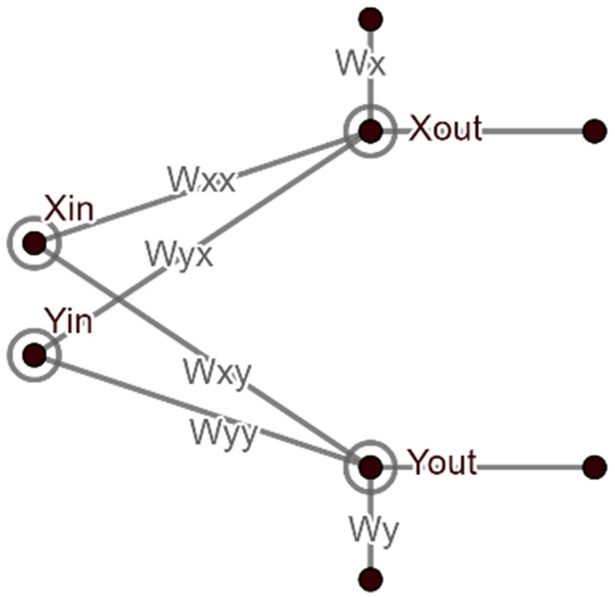
A set of weights for the neural network is selected for a given fractal attractor, which will approximate the attractor. The neural network used in the present paper consists of two input units, namely $X_{in}$, $Y_{in}$, two output units, $X_{out}, Y_{out}$ and six weights per transformation (IFS) represent a function with a homogeneous recursive function system state (Figure 1). This number of inputs, output units and weights may change for other cases of IFS. The transformation is selected randomly. All input neurons receive an $X_{in}$ and $Y_{in}$ coordinate of each point of the fractal image, the first one for x coordinate and the other neuron for y coordinate for each transform. The neurons return as $X_{out}$ and $Y_{out}$ output, consisting of different activation functions with bias.

5. Activation Function

The activation function is defined by ϕ(v) to smooth out the data to fit the purpose for which the network is designed and determines the neuron’s output based on input and weight values.

Many types of these activation functions can be classified with respect to their domain, such as:

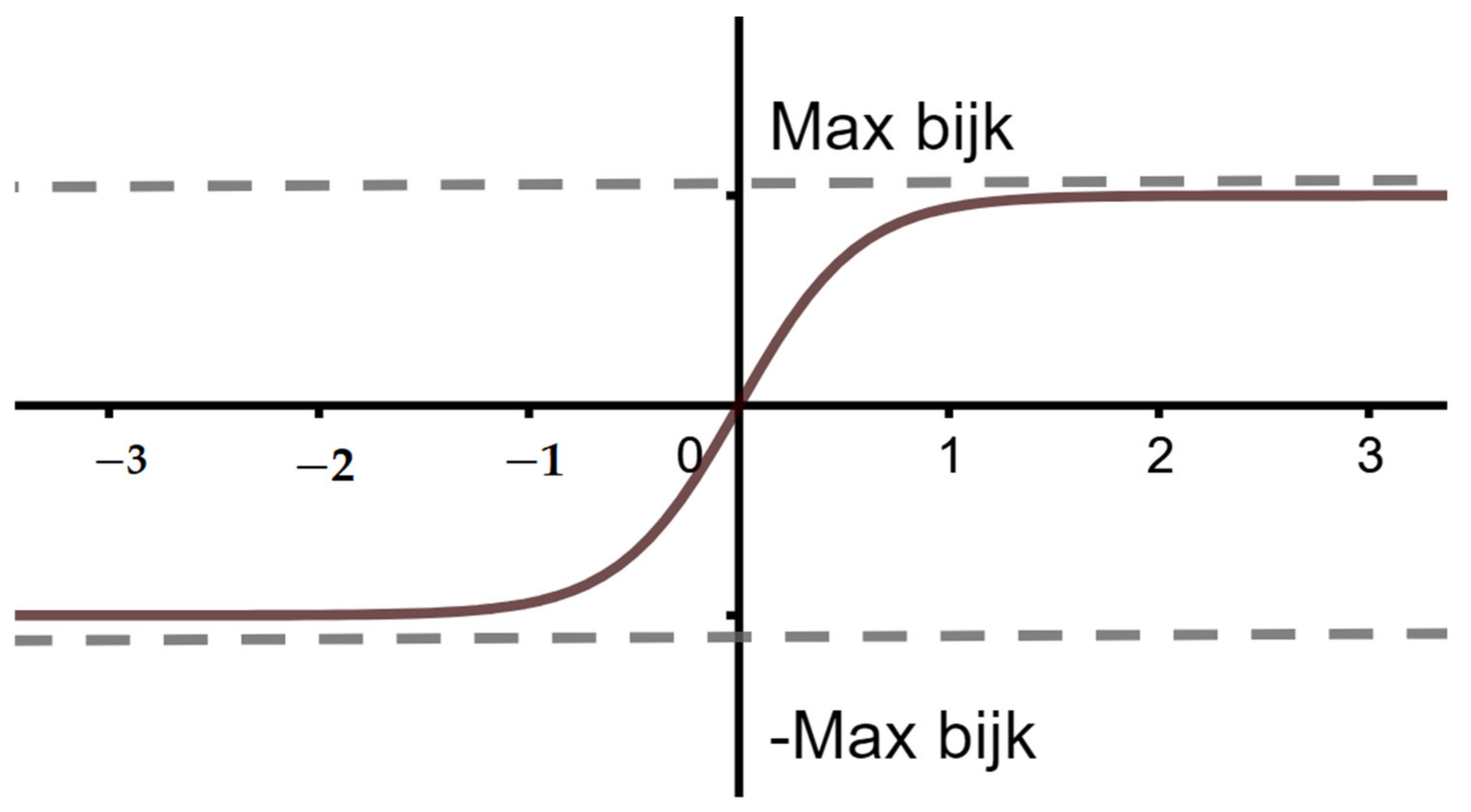
• Logistic function $\varphi \left(v\right)=\frac{1}{1+e^{-av}}$ where domain is $\left[0, 1\right]$.
• Hyperbolic tangent $\varphi \left(v\right)=\frac{1-e^{-av}}{1+e^{-av}}$ and algebraic sigmoid function $\frac{v}{\sqrt{1+v^2}}$ where domain is $\left[-1,1\right]$.

In this equation, a is the logistic growth rate. The present paper will constrict on sigmoid activation functions, which are helpful to fractals coding.

The fractal image can be divided into three parts with respect to the coefficients of IFS.

5.1. Learning Rate with Positive Coefficients of IFS

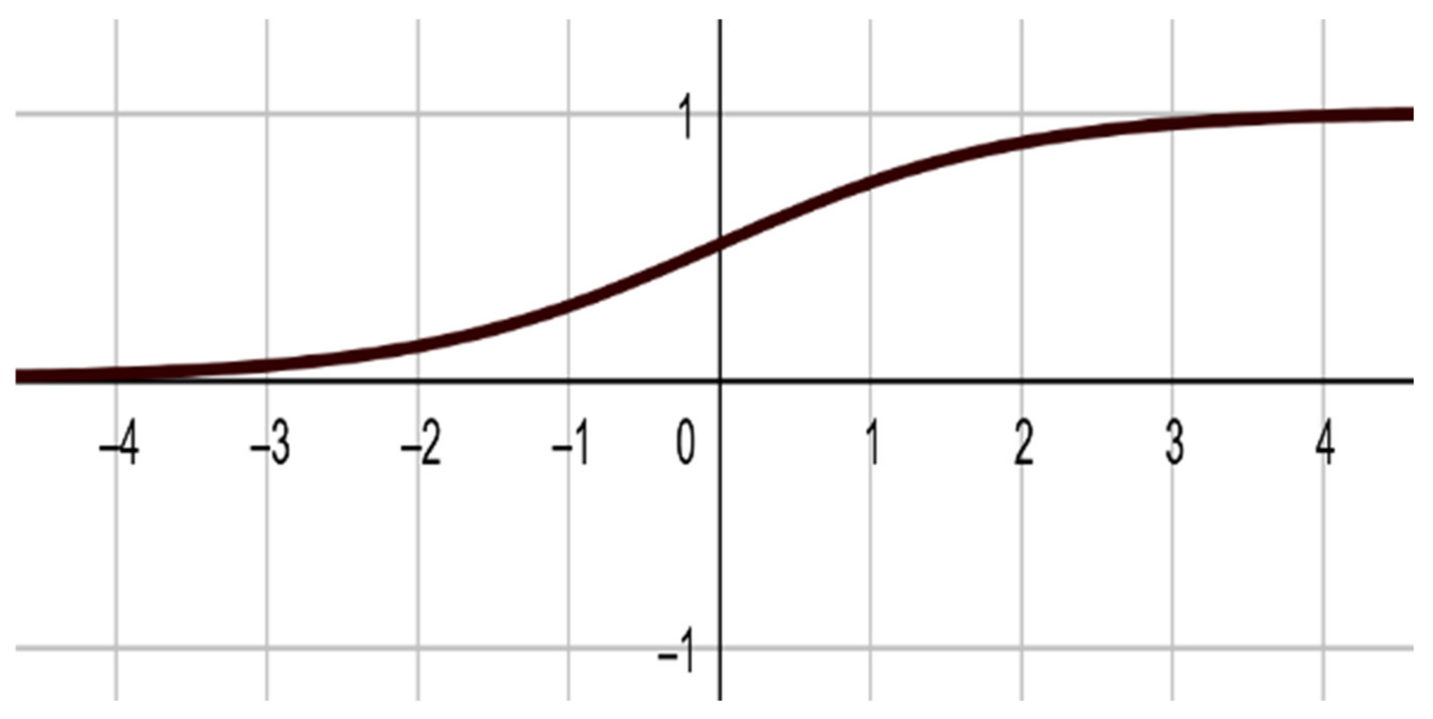
The neural network’s output for this kind of IFS consists of two units as a calculation of two input units and six weights for all transform (IFS) that represent a scalar function. The iterated function is randomly selected. All input neuron units receive a single coordinate of each point of the fractal image, one neuron for the x coordinate and the other for the y coordinate for each transform. Each output neuron returns as x and y output, consisting of Sigmoid function [7,9] with bias (Figure 2).

The two equations of X and Y output are given as

$$X_{out}=\frac{1}{1+e^{-aW{X}_{in}}}$$

and

$$Y_{out}=\frac{1}{1+e^{-aW{Y}_{in}}},$$

where $a$ is the growth rate,

$$W{X}_{in}=XinWxx+YinWyx+Wx,$$

and

$$W{Y}_{in}=X_{in}Wxy+Y_{in}Wyy+Wy$$

is the weight function from i input to j output neuron, and W_i is the bias of i input neuron. An image is obtained at the end of this iterated operation for many points with random iterations. This image differs from the image we aimed to find in the system (IFS). Thus, the neural network weights must be updated to obtain an improved approximation of the target image.

This change of weights depends on the amount of difference between the two images. This difference is measured to get the error function, which should decrease with each update of weight values.

The error function used to compare the two fractal attractors is the Hausdorff distance [1,11].

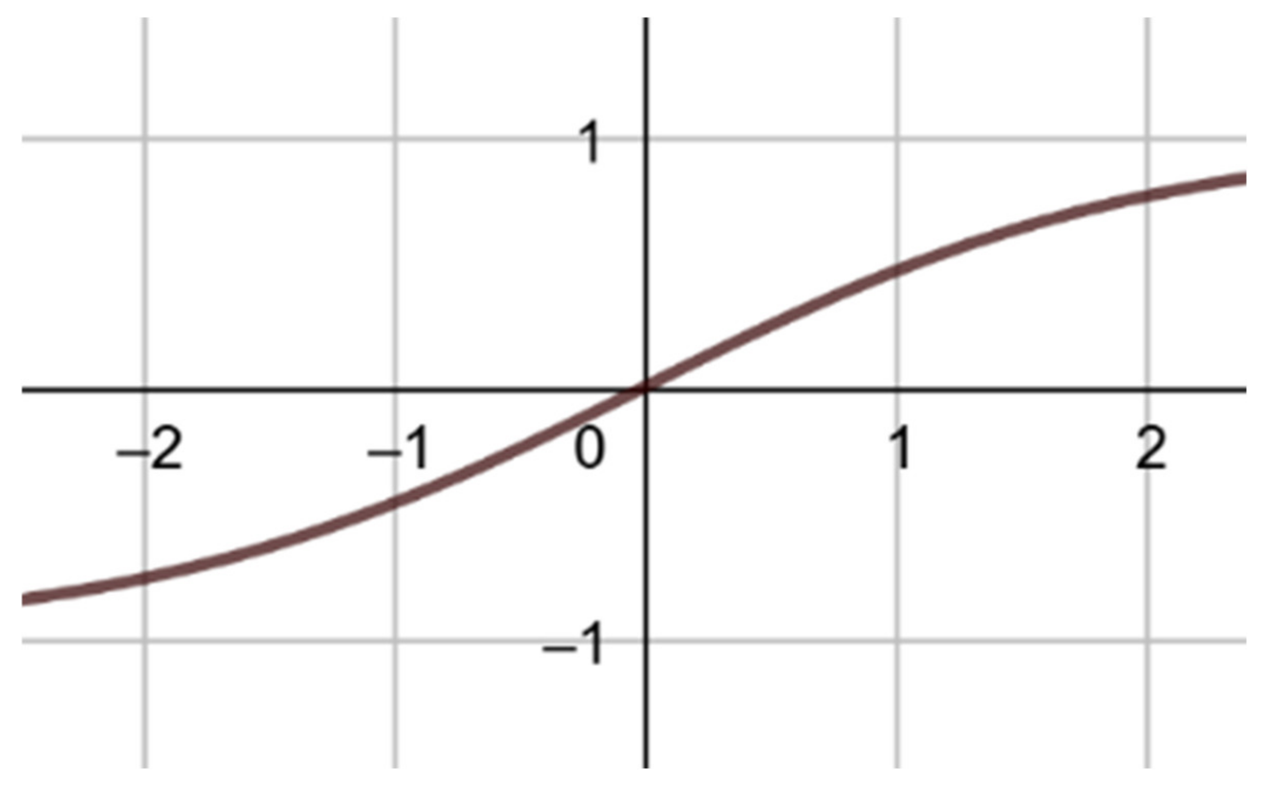
5.2. Learning Rate with Positive and Negative Coefficients of IFS

The same neural network and procedure will be used for this kind of IFS. The X and Y output neuron consist of a TanSigmoid function with bias [7,9] (Figure 3).

The two equations of x and y outputs are given by:

$$X_{out}=\frac{1-e^{-aW{X}_{in}}}{1+e^{-aW{X}_{in}}} \mathrm{and} Y_{\mathrm{out}}=\frac{1-e^{-aW{Y}_{in}}}{1+e^{-aW{Y}_{in}}}$$

With the same symbols used in the first kind of IFS and b_ijk are the coefficients of IFS, i = 1, 2, …, n, where n is the number of IFS, j = 1, 2, and k = 1, 2, 3.

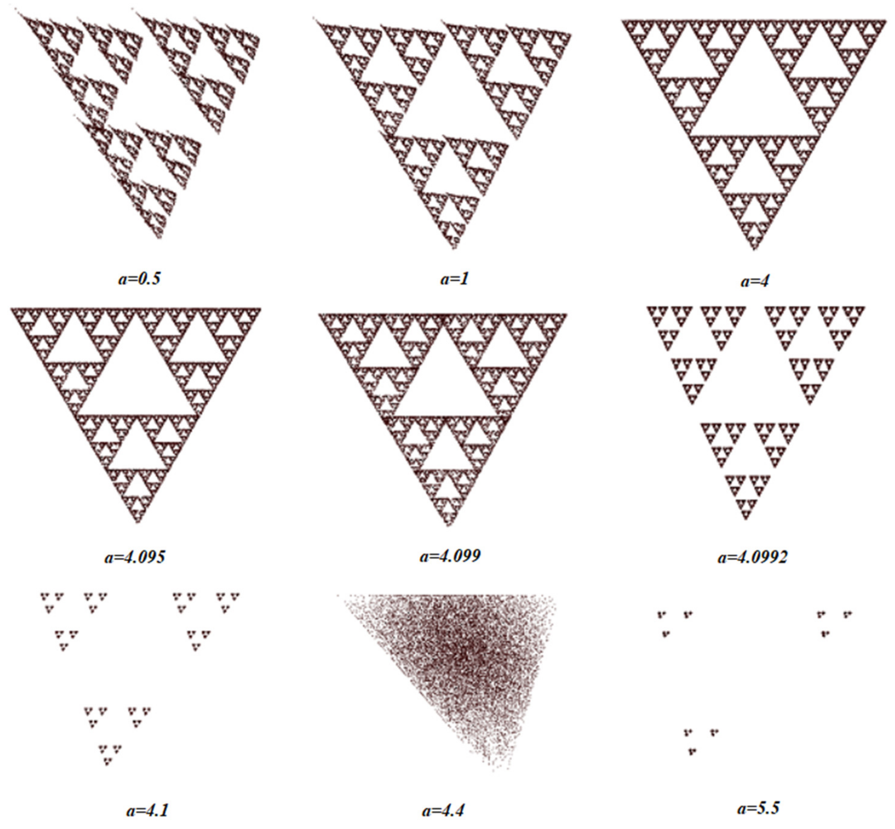
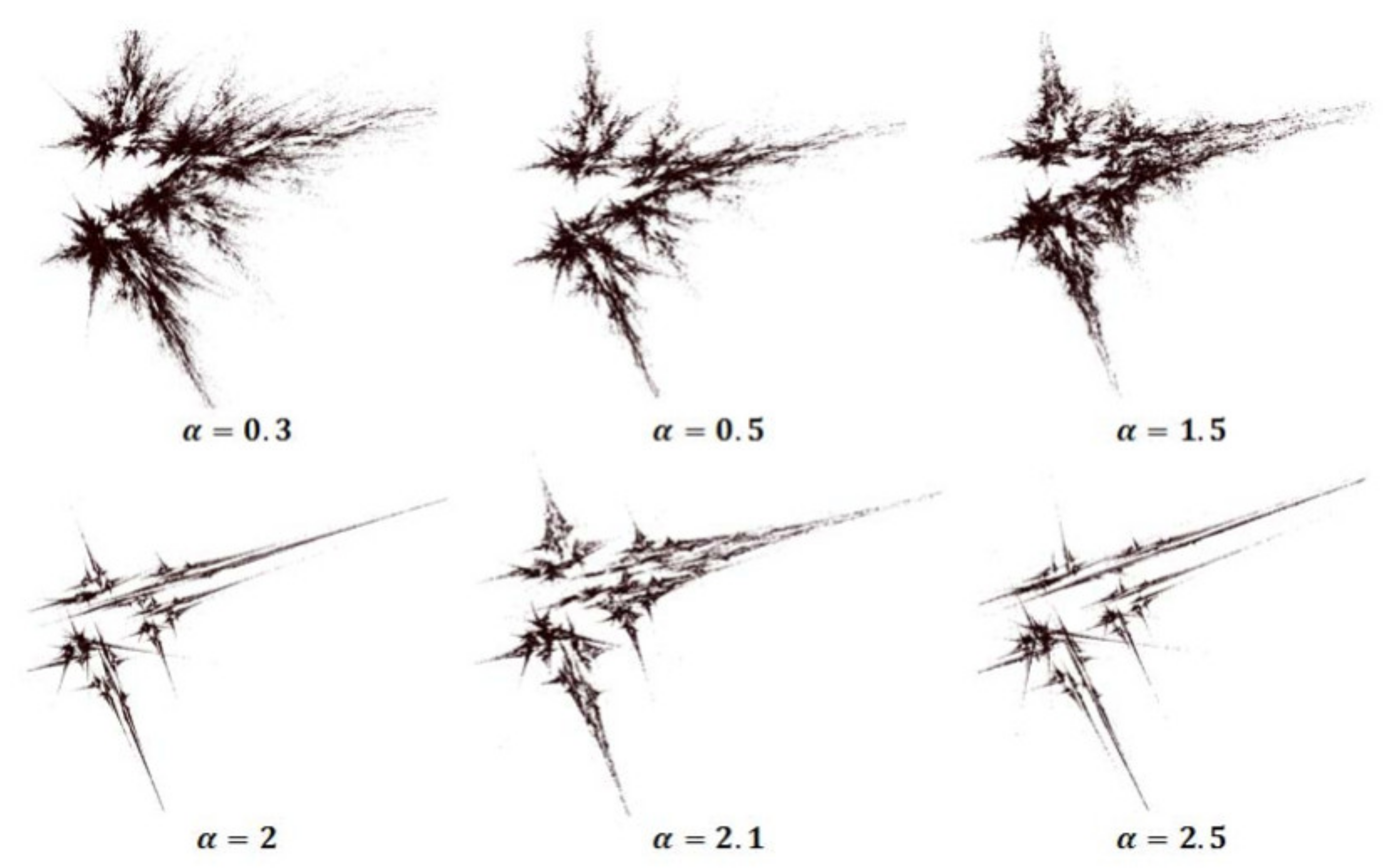
Figure 4, Figure 5 and Figure 6 show some last fractal images of neural networks with sigmoid, and tan sigmoid function for different growth rates. The same error function of the first kind of fractal will be used in this kind of fractal.

5.3. Learning Rate with Coefficients of IFS b_ij > 1

The activation function for this kind of fractal will be the same activation function for the first kind if b_ij is positive and the same activation function for the second kind if bij is positive and negative with a small change for the two cases (Figure 3 and Figure 7).

The two equations of x and y outputs are given as

$$X_{out}=\frac{max\left\{b_{ijk}\right\}}{1+e^{-aW{X}_{in}}} \mathrm{and} Y_{out}=\frac{max\left\{b_{ijk}\right\}}{1+e^{-aW{Y}_{in}}}$$

or

$$X_{out}=max\left\{b_{ijk}\right\}\frac{1-e^{-aW{X}_{in}}}{1+e^{-aW{X}_{in}}} \mathrm{and} Y_{out}=max\left\{b_{ijk}\right\}\frac{1-e^{-aW{Y}_{in}}}{1+e^{-aW{Y}_{in}}}.$$

The same symbols are used in the first and second kinds of IFS.

6. Future Work

The present paper focused on the congenial activation function for different kinds of fractals. Some results with different growth rates are introduced for all kinds. Some values of growth rate increase the speed of convergence of the neural network to the target fractal image of each kind of fractal. The relation between growth rate and activation functions related to fractal image coding remains an open problem.