Finite-Time Projective Synchronization and Parameter Identification of Fractional-Order Complex Networks with Unknown External Disturbances

Abstract

This paper is devoted to exploring the finite-time projective synchronization (FTPS) of fractional-order complex dynamical networks (FOCDNs) with unknown parameters and external disturbances. Based on the stability theory of fractional-order differential systems, synchronization criteria between drive-response networks were obtained and both the uncertain parameters and external disturbances were identified or conquered simultaneously. Moreover, the upper limit of the settling-time function was obtained. Finally, a numerical example was given to verify the effectiveness of the results.

1. Introduction

A. Previous Works

In recent years, many efforts have been devoted to the synchronization and stability of complex networks, and the relevant research has yielded beneficial results [1,2,3,4,5,6,7,8,9,10,11,12,13,14,15]. Various types of integer-order system synchronizations have been proposed, such as drive-response synchronization, exponential synchronization, lag synchronization, projective synchronization, cluster synchronization, double compound combination synchronization, hybrid synchronization, and so on.

Although there are many results about the synchronization of complex networks, most efforts have been devoted to integer-order networks. In contrast to integer-order networks, synchronization of FOCDNs has recently become a hot research area, owing to the fact that fractional-order systems can more correctly capture actual behavior characteristics due to their memory and genetic properties. Hence, some remarkable results with respect to the synchronization of FOCDNs have been addressed recently, see [16,17,18,19,20,21]. In particular, Li et al. [22] focused on the global exponential synchronization problem for fractional-order complex dynamical networks with derivative couplings and impulse effects. Li et al. [23] committed to exploring the finite-time synchronization problem of FOCDNs with time-varying delay and external interference by means of a discontinuous feedback controller. In [24], A. Pratap et al. researched finite-time synchronization of FOCDNs with time-varying delays by using some inequalities. In [25], Zheng et al. studied synchronization of fractional-order complex-valued coupled neural networks with time varying coupling strengths. Li et al. [26] researched the problem with respect to finite-time synchronization for FOCDNs via a hybrid feedback control. Modified projective function synchronization of non-linear distributive FOCDNs has been investigated in [27]. Yang et al. [28] focused on the global exponential cluster synchronization of switched FOCDNs with switching topology and impulses. The impulsive synchronization of a fractional-order complex-variable network was investigated in [29].

On the other hand, there are many uncertain factors that affect or destroy the synchronization process of real complex networks, such as delay, unknown system parameters, uncertain network structures, uncertain external disturbances, and so on. Therefore, the consideration of unknown system parameters and uncertain external disturbances effects in the synchronization issues of FOCDNs is more significant [30,31,32]. Pei et al. [33] studied both local and global synchronizations of fractional-order nonlinearly coupled complex networks with time delays and unknown external disturbances. Chen et al. investigated the parameter identification problem for FOCDNs utilizing the adaptive control technique and the stability theorem of fractional-order systems in [34]. Li et al. [35] considered finite-time synchronization and the parameter identification problem of uncertain FOCDNs. In [36] P. Selvaraj discussed the combined problems of cluster synchronization and disturbance rejection for a family of FOCDNs subject to coupling delays, unknown uncertainty, and disturbances. Du [37] used the stability theory of fractional-order differential systems to investigate the problem of modified function projective synchronization between two FOCDNd with unknown parameters and unknown bounded external disturbances. Although many synchronizations of FOCDNs with unknown external disturbances and unknown parameters have been proposed in previous papers, unfortunately, the FTPS problem of two uncertain FOCDNs with coupling delays has not been mentioned in the existing literature. Hence, we will address this problem, in this paper.

B. Main Contributions

The significant contributions of this research are outlined below in comparison to current results:

(1)

The problem about FTPS and parameter identification of FOCDNs with coupling delays and unknown external disturbances was studied in this work. By using the analysis techniques of fractional calculation, some more practical controllers were obtained to ensure FTPS between the considered FOCDNs.

(2)

The controllers could not only estimate unknown parameters in the networks, but also overcome unknown bounded disturbances. Simultaneously, the setting time for synchronization could also be accurately estimated.

This paper is organized as follows. Section 2 introduces the network model and provides the necessary definitions, lemmas, and hypotheses. Section 3 discusses the FTPS of FOCDNs. In Section 4, you will find examples and simulations. Finally, in Section 5, conclusions are formed.

2. Preliminaries

In this section, we review several fundamental definitions and introduce a few lemmas.

Definition 1 ([38]).

The Caputo fractional derivative of order $q$for a function$g(t)$is defined by

$${}_{t_0}{}^{C}D_t^{q}g(t)=\frac{1}{\Gamma (n-q)}{\displaystyle {\int }_{t_0}^t\frac{g^{(n)}(s)}{{(t-s)}^{q-n+1}}}ds,$$

where$\Gamma (·)$is the gamma function,$t\ge t_0$,$n$is a positive integer,$n-1<q<n$. Especially, when$0<q<1$,

$${}_{t_0}{}^{C}D_t^{q}g(t)=\frac{1}{\Gamma (1-q)}{\displaystyle {\int }_{t_0}^t\frac{g^{\prime }(s)}{{(t-s)}^q}}ds,$$

also, the Riemann–Liouville (RL) definition of fractional operator is given as

$${}_{t_0}{}^{C}D_t^{q}g(t)=\frac{1}{\Gamma (n-q)}\frac{d^n}{d{t}^n}{\displaystyle {\int }_{t_0}^t\frac{g(s)}{{(t-s)}^{q-n+1}}}ds.$$

Lemma 1.

Ref ([39]). For any vectors$x,y\in R^n$there is a positive definite matrix$Q\in R^{n\times n}$and the following matrix inequality holds:

$$2x^{T}y \le x^{T}Qx+y^T{Q}^{-1}y.$$

Lemma 2.

Ref ([40]). If$g(t)\in C^1 \left([t_{0,}+\infty ),R\right),$then for$0<\forall q<1,$

$${}_{t_0}{}^{C}D_t^q\left|g(t)\right|\le sign(g(t)){}_{t_0}{}^{C}D_t^{q}g(t),$$

holds almost everywhere, where$sign(·)$denotes the sign function.

Lemma 3.

Ref ([41]). Let$x(t)\in R^n$be a differentiable vector function. Then, for any time instant$t\ge 0,$

$$\frac{1}{2}{}_{t_0}{}^{C}D_t^q(x^T(t)x(t))\le x^T(t){}_{t_0}{}^{C}D_t^{q}x(t),$$

where$0<q<1$is the fractional order.

Lemma 4.

Ref ([23]). Suppose$V:D\to R$is a continuous function, which satisfies the following conditions:

(1)

V(t) is positive definite;

(2)

$\exists \mu \in R^{+}$such that

$${}_{t_0}{}^{C}D_t^{q}V(t)\le -\mu ,t\in [t_{0,}\infty ),$$

then$V(t)$fulfils

$$V(t)\le V(t_0)-\frac{\mu {(t-t_0)}^q}{\Gamma (1+q)},t_0\le t\le T(t_0),$$

and$V(t)\equiv 0$for$t\ge T(t_0)$. Moreover,$T(t_0)$is the settling-time function,

$$T(t_0)=t_0+{(\frac{V(t_0)\Gamma (1+q)}{\mu })}^{\frac{1}{q}},$$

and$T(t_0)$is continuous.

Consider the following nonlinear FOCDN consisting of $N$ identical nodes

$$D_{*}^q{x}_i(t)=f\left(x_i\right)+F\left(x_i\right)\theta +c{\displaystyle \sum _{j=1}^N{b}_{ij}H{x}_j(t)}+\overline{c}{\displaystyle \sum _{j=1}^N{\overline{b}}_{ij}\overline{H}{x}_j(t-\tau )},$$

(1)

where $x_i^{}(t)={(x_{i1}^{}(t),x_{i2}^{}(t),\cdot \cdot \cdot ,x_{in}^{}(t))}^T\in R^n$ denotes the state vector of the $i$th node, $f:R^n\to R^n$ is a continuously differentiable vector function, $F:R^n\to R^{n\times m}$ is a function matrix, $\theta \in R^m$ is a parameter vector, $c$ and $\overline{c}$ are the coupling strengths, $\tau >0$ is an unknown coupling delay, $0<q<1$ denotes fractional order. $H=diag({\epsilon }_1,{\epsilon }_2,\cdots ,{\epsilon }_n)>0$ and $\overline{H}=diag({\overline{\epsilon }}_1,{\overline{\epsilon }}_2,\cdots ,{\overline{\epsilon }}_n)>0$ are inner-coupling matrices. $B={(b_{ij})}_{N\times N}\in R^{N\times N}$ and $\overline{B}={(b_{ij})}_{N\times N}\in R^{N\times N}$ are the zero-row sum of the outer coupling matrices, which represents the topological structure. $b_{ij}\ne 0$ and ${\overline{b}}_{ij}\ne 0$ if there exists a direct link from node $i$ to node $j$, otherwise $b_{ij}={\overline{b}}_{ij}=0$.

To realize the FTPS between two FOCDNs, we refer to model in (1) as the drive network, and our response network is written as

$$D_{*}^q{y}_i=f\left(y_i\right)+F\left(y_i\right)\widehat{\theta }+c{\displaystyle \sum _{j=1}^N{b}_{ij}H{y}_j(t)}+\overline{c}{\displaystyle \sum _{j=1}^N{\overline{b}}_{ij}\overline{H}{y}_j(t-\tau )}+{\mathsf{\Theta }}_i^{}(t)+u_i(t),$$

(2)

where $u_i(t)$ is the control input applied to node $i$, $\widehat{\theta }$ is the estimated parameter vector, ${\mathsf{\Theta }}_i^{}(t)$ is the disturbance, and the other symbols are the same as above.

Definition 2.

If there is a matrix Λ such that

$$\underset{t\to t_1}{\lim }{\Vert e_i(t)\Vert }_1=\underset{t\to t_1}{\lim }{\Vert y_i^{}(t)-\mathsf{\Lambda }{x}_i(t)\Vert }_1=\underset{t\to t_1}{\lim }{\Vert \widehat{\theta }(t)-\theta \Vert }_1=0,$$

(3)

and ${\Vert y_i^{}(t)-\mathsf{\Lambda }{x}_i(t)\Vert }_1={\Vert \widehat{\theta }(t)-\theta \Vert }_1\equiv 0$ if $t>t_1^{}$, $t_1^{}$ is called the setting time, where $\mathsf{\Lambda }=diag({\kappa }_1,{\kappa }_1,\cdots ,{\kappa }_1)$ is an n-order diagonal matrix, ${\kappa }_i\in R$, then the network (1) and (2) are FTPS.

We know from Definition 2

$$D_{*}^q{e}_i(t)=D_{*}^q(y_i(t)-\mathsf{\Lambda }{x}_i(t))=D_{*}^q{y}_i(t)-D_{*}^q(\mathsf{\Lambda }{x}_i(t))$$

$$\begin{array}{l}=f\left(y_i\right)+F\left(y_i\right)\widehat{\theta }+c{\displaystyle \sum _{j=1}^N{b}_{ij}H{y}_j(t)}+\overline{c}{\displaystyle \sum _{j=1}^N{\overline{b}}_{ij}\overline{H}{y}_j(t-\tau )}\\ \hspace{1em}\hspace{1em}\hspace{1em}\hspace{1em}+{\mathsf{\Theta }}_i^{}(t)+u_i(t)-D_{*}^q(\mathsf{\Lambda }{x}_i(t))\end{array}$$

$$\begin{array}{l}=F\left(y_i\right)[\widehat{\theta }(t)-\theta ]+c{\displaystyle \sum _{j=1}^N{b}_{ij}H{e}_j(t)}+\overline{c}{\displaystyle \sum _{j=1}^N{\overline{b}}_{ij}\overline{H}{e}_j(t-\tau )}+{\mathsf{\Theta }}_i^{}(t)\\ +c{\displaystyle \sum _{j=1}^N{b}_{ij}H\mathsf{\Lambda }{x}_j(t)}+\overline{c}{\displaystyle \sum _{j=1}^N{\overline{b}}_{ij}\overline{H}\mathsf{\Lambda }{x}_j(t-\tau )}\\ -D_{*}^q(\mathsf{\Lambda }{x}_i(t))+F\left(y_i\right)\theta +f\left(y_i\right)+u_i(t).\end{array}$$

(4)

Assumption 1.

$\exists {\varpi }_i^{*}\in R^{+}$such that the time-varying disturbances${\mathsf{\Theta }}_i^{}(t)=\phi (t)sign(e_i(t))$are bounded, i.e.,$\left|\phi (t)\right|\le {\varpi }_i^{*}<\infty .$

3. Main Results

We investigated the FTPS of two complex networks in this part. To achieve synchronization between the two networks, we designed the controllers as follows:

$$u_i(t)=v_i(t)+w_i(t),$$

(5)

where

$$\begin{array}{l}{v}_i(t)=-c{\displaystyle \sum _{j=1}^N{b}_{ij}H\mathsf{\Lambda }{x}_j(t)}-\overline{c}{\displaystyle \sum _{j=1}^N{\overline{b}}_{ij}\overline{H}\mathsf{\Lambda }{x}_j(t-\tau )}\\ +D_{*}^q(\mathsf{\Lambda }{x}_i(t))-F\left(y_i\right)\theta -f\left(y_i\right),\end{array}$$

$$\begin{array}{l}{w}_i(t)=-{\widehat{\varpi }}_i(t)sign(e_i(t))-{\widehat{\eta }}_i(t)e_i(t)-{\vartheta }_{i}sign(e_i(t))\\ -\frac{1}{2}sign(e_i(t))e_i^T(t-\tau )e_i^{}(t-\tau ),\end{array}$$

$$D_{*}^q\widehat{\theta }(t)=-{\Vert F^T\left(y_i\right)\Vert }_1{e}_{\theta }(t)-\mu sign(e_{\theta }(t)),$$

(6)

$$D_{*}^q{\widehat{\varpi }}_i(t)=q_i{[sign(e_i^{}(t))]}^{T}sign(e_i(t)),$$

(7)

$$D_{*}^q{\widehat{\eta }}_i(t)=r_i{[sign(e_i^{}(t))]}^T{e}_i(t).$$

(8)

where $e_{\theta }(t)=\widehat{\theta }(t)-\theta$ and $q_i>0,r_i>0,{\vartheta }_i>0$ are arbitrary positive constants.

Theorem 1.

Assume that the above assumption, Assumption 1, is tenable. If the following inequalities hold,

$$c\epsilon {\displaystyle \sum _{j=1}^N{b}_{ij}-{\eta }_i^{*}}\le 0,$$

(9)

$$\mu ={\vartheta }_i-\frac{1}{2}{\stackrel{-}{c}}^2{\lambda }_{\max }\left(P^{T}P\right).$$

(10)

where$\epsilon =\max \left\{{\epsilon }_i,i=1,2,\cdots n\right\}$then taking appropriate${\eta }_i{}^{*}$and${\vartheta }_i^{}$such that the drive networks (1) and response networks (2) are said to achieve FTPS via the controllers $u_i(t)$, FTPS will be realized in finite-time$t_1$, and the settling time is

$$t_1=t_0+{(\frac{V(t_0)\Gamma (1+q)}{\mu })}^{\frac{1}{q}},$$

where$V(t_0)={\displaystyle \sum _{i=1}^N{\Vert e_i(t_0)\Vert }_1+}{\Vert e_{\theta }(t_0)\Vert }_1+\frac{1}{2}{\displaystyle \sum _{i=1}^N\frac{1}{q_i}{\tilde{\varpi }}_i^2(t_0)+}\frac{1}{2}{\displaystyle \sum _{i=1}^N\frac{1}{r_i}{\tilde{\eta }}_i^2(t_0)}$,$e_i(t_0)$,$e_{\theta }(t_0)$,${\tilde{\varpi }}_i^{}(t_0)$,${\tilde{\eta }}_i^{}(t_0)$are the initial values of$e_i(t)$,$e_{\theta }(t)$,${\tilde{\varpi }}_i^{}(t)$,${\tilde{\eta }}_i^{}(t)$respectively.

Proof. 

We construct the Lyapunov function as follows

$$V(t)={\displaystyle \sum _{i=1}^N{\Vert e_i(t)\Vert }_1+}{\Vert e_{\theta }(t)\Vert }_1+\frac{1}{2}{\displaystyle \sum _{i=1}^N\frac{1}{q_i}{\tilde{\varpi }}_i^2(t)+}\frac{1}{2}{\displaystyle \sum _{i=1}^N\frac{1}{r_i}{\tilde{\eta }}_i^2(t)},$$

where ${\tilde{\varpi }}_i^{}(t)={\varpi }_i^{*}-{\widehat{\varpi }}_i^{}(t),{\tilde{\eta }}_i^{}(t)={\eta }_i^{*}-{\widehat{\eta }}_i^{}(t)$□

It follows from Lemmas 2 and 3 that we have

$$\begin{array}{ll}\hfill D_{*}^{q}V(t)& =D_{*}^q({\displaystyle \sum _{i=1}^N{\Vert e_i(t)\Vert }_1+}{\Vert e_{\theta }(t)\Vert }_1+\frac{1}{2}{\displaystyle \sum _{i=1}^N\frac{1}{q_i}{\tilde{\varpi }}_i^2(t)+}\frac{1}{2}{\displaystyle \sum _{i=1}^N\frac{1}{r_i}{\tilde{\eta }}_i^2(t)})\hfill \\ & =D_{*}^q({\displaystyle \sum _{i=1}^N{\displaystyle \sum _{k=1}^m\left|e_{ik}(t)\right|}+}{\displaystyle \sum _{h=1}^m\left|{\widehat{\theta }}_h(t)-{\theta }_h\right|})+{\displaystyle \sum _{i=1}^N\frac{1}{q_i}{\tilde{\varpi }}_i^{}(t)D_{*}^q{\tilde{\varpi }}_i^{}(t)}\hfill \\ & +{\displaystyle \sum _{i=1}^N\frac{1}{r_i}{\tilde{\eta }}_i^{}(t)D_{*}^q}{\tilde{\eta }}_i^{}(t)\hfill \end{array}$$

$$\begin{array}{l}\le {\displaystyle \sum _{i=1}^N{\displaystyle \sum _{k=1}^n[sign}(e_{ik}^{}(t)){]}^T{D}_{*}^q{e}_{ik}(t)}+{\displaystyle \sum _{h=1}^m{[sign({\widehat{\theta }}_h(t)-{\theta }_h)]}^T{D}_{*}^q({\widehat{\theta }}_h(t)-{\theta }_h)}\\ \hspace{1em}+{\displaystyle \sum _{i=1}^N\frac{1}{q_i}{\tilde{\varpi }}_i^{}(t)D_{*}^q{\tilde{\varpi }}_i^{}(t)+}{\displaystyle \sum _{i=1}^N\frac{1}{r_i}{\tilde{\eta }}_i^{}(t)D_{*}^q}{\tilde{\eta }}_i^{}(t)\end{array}$$

$$\begin{array}{l}={\displaystyle \sum _{i=1}^N{[sign(e_i^{}(t))]}^T{D}_{*}^q{e}_i(t)}+{[sign(e_i^{}(t))]}^T{D}_{*}^q(e_{\theta }(t))\\ \hspace{1em}+{\displaystyle \sum _{i=1}^N\frac{1}{q_i}{\tilde{\varpi }}_i^{}(t)D_{*}^q{\tilde{\varpi }}_i^{}(t)+}{\displaystyle \sum _{i=1}^N\frac{1}{r_i}{\tilde{\eta }}_i^{}(t)D_{*}^q}{\tilde{\eta }}_i^{}(t)\end{array}$$

$$\begin{array}{l}={\displaystyle \sum _{i=1}^N{[sign(e_i^{}(t))]}^T[F\left(y_i\right)e_{{\theta }_i}(t)+c{\displaystyle \sum _{j=1}^N{b}_{ij}H{e}_j(t)}}\\ \hspace{1em}+\overline{c}{\displaystyle \sum _{j=1}^N{\overline{b}}_{ij}\overline{H}{e}_j(t-\tau )}+{\mathsf{\Theta }}_i^{}(t)-{\widehat{\varpi }}_i^{}(t)sign(e_i(t))-{\widehat{\eta }}_i(t)e_i(t)\\ \hspace{1em}-\frac{1}{2}sign(e_i(t))e_i^T(t-\tau )e_i^{}(t-\tau )-{\vartheta }_{i}sign(e_i(t))]\\ \hspace{1em}+[{(sign(e_i^{}(t))]}^T[-{\Vert F^T\left(y_i\right)\Vert }_1(e_{\theta }(t))-\mu sign(e_{\theta }(t))]\\ \hspace{1em}-{\displaystyle \sum _{i=1}^N\frac{1}{q_i}({\varpi }_i^{*}-{\widehat{\varpi }}_i^{}(t))D_{*}^q{\widehat{\varpi }}_i^{}(t)}-{\displaystyle \sum _{i=1}^N\frac{1}{r_i}({\eta }_i^{*}-{\widehat{\eta }}_i^{}(t))D_{*}^q}{\widehat{\eta }}_i^{}(t)\end{array}$$

$$\begin{array}{l}\le {\displaystyle \sum _{i=1}^N{[sign(e_i^{}(t))]}^{T}F\left(y_i^{}\right)}(e_{\theta }(t))+c{\displaystyle \sum _{i=1}^N{[sign(e_i^{}(t))]}^T{b}_{ij}^{}H{e}_j^{}(t)}\\ \hspace{1em}+\overline{c}{\displaystyle \sum _{i=1}^N{\displaystyle \sum _{j=1}^N{[sign(e_i^{}(t))]}^T{\overline{b}}_{ij}^{}\overline{H}{e}_j^{}(t-\tau )}}+{\displaystyle \sum _{i=1}^N{[sign(e_i^{}(t))]}^T{\mathsf{\Theta }}_i^{}(t)}\\ \hspace{1em}-{\displaystyle \sum _{i=1}^N{[sign(e_i^{}(t))]}^T{\widehat{\varpi }}_i^{}(t)sign(e_i^{}(t))}-{\displaystyle \sum _{i=1}^N{[sign(e_i^{}(t))]}^T{\widehat{\eta }}_i^{}(t)e_i^{}(t)}\\ \hspace{1em}-{\displaystyle \sum _{i=1}^N{[sign(e_i^{}(t))]}^T\frac{1}{2}sign(e_i^{}(t))e_i^T(t-\tau )e_i^{}(t-\tau )}\\ \hspace{1em}-{\displaystyle \sum _{i=1}^N{[sign(e_i^{}(t))]}^T{\vartheta }_i^{}sign(e_i^{}(t))}-{[sign(e_i^{}(t))]}^T{\Vert F^T\left(y_i^{}\right)\Vert }_1(e_{\theta }(t))\\ \hspace{1em}-\mu {[sign(e_i^{}(t))]}^{T}sign(e_{\theta }(t))-{\displaystyle \sum _{i=1}^N\frac{1}{q_i^{}}({\varpi }_i^{*}-{\widehat{\varpi }}_i^{}(t))D_{*}^q{\widehat{\varpi }}_i^{}(t)}\\ \hspace{1em}-{\displaystyle \sum _{i=1}^N\frac{1}{r_i^{}}({\eta }_i^{*}-{\widehat{\eta }}_i^{}(t))D_{*}^q{\widehat{\eta }}_i^{}(t)}\end{array}$$

$$\begin{array}{l}\le {\Vert F\left(y_i\right)\Vert }_1{\Vert e_{\theta }(t)\Vert }_1+c{\displaystyle \sum _{i=1}^N{\displaystyle \sum _{j=1}^N{[sign(e_i^{}(t))]}^T{b}_{ij}H{e}_j(t)}}\\ \hspace{1em}+\overline{c}{\displaystyle \sum _{i=1}^N{\displaystyle \sum _{j=1}^N{[sign(e_i^{}(t))]}^T{\overline{b}}_{ij}\overline{H}{e}_j(t-\tau )}}+{\displaystyle \sum _{i=1}^N{[sign(e_i^{}(t))]}^T{\mathsf{\Theta }}_i^{}(t)}\\ \hspace{1em}-{\displaystyle \sum _{i=1}^N{[sign(e_i^{}(t))]}^T{\widehat{\varpi }}_i^{}(t)sign(e_i(t))}-{\displaystyle \sum _{i=1}^N{[sign(e_i^{}(t))]}^T{\widehat{\eta }}_i(t)e_i(t)}\\ \hspace{1em}-\frac{1}{2}{\displaystyle \sum _{i=1}^N{e}_i^T(t-\tau )e_i^{}(t-\tau )}-{\displaystyle \sum _{i=1}^N{[sign(e_i^{}(t))]}^T{\vartheta }_{i}sign(e_i(t))}\\ \hspace{1em}-{[sign(e_i^{}(t))]}^T{\Vert F^T\left(y_i\right)\Vert }_1(e_{\theta }(t))-\mu {[sign(e_i^{}(t))]}^{T}sign(e_{\theta }(t))\\ \hspace{1em}-{\displaystyle \sum _{i=1}^N\frac{1}{q_i}({\varpi }_i^{*}-{\widehat{\varpi }}_i^{}(t))D_{*}^q{\widehat{\varpi }}_i^{}(t)}-{\displaystyle \sum _{i=1}^N\frac{1}{r_i}({\eta }_i^{*}-{\widehat{\eta }}_i^{}(t))D_{*}^q}{\widehat{\eta }}_i^{}(t)\end{array}$$

$$\begin{array}{l}=c{\displaystyle \sum _{i=1}^N{\displaystyle \sum _{j=1}^N{b}_{ij}{[sign(e_i^{}(t))]}^{T}H{e}_j(t)}}+\overline{c}{\displaystyle \sum _{i=1}^N{\displaystyle \sum _{j=1}^N{\overline{b}}_{ij}{[sign(e_i^{}(t))]}^T\overline{H}{e}_j(t-\tau )}}\\ \hspace{1em}+{\displaystyle \sum _{i=1}^N{[sign(e_i^{}(t))]}^T}\phi (t)sign(e_i(t))-\frac{1}{2}{\displaystyle \sum _{i=1}^N{e}_i^T(t-\tau )e_i^{}(t-\tau )}\\ \hspace{1em}-{\displaystyle \sum _{i=1}^N{[sign(e_i^{}(t))]}^T}{\vartheta }_{i}sign(e_i(t))-\mu {[sign(e_i^{}(t))]}^{T}sign(e_{\theta }(t))\\ \hspace{1em}-{\displaystyle \sum _{i=1}^N{[sign(e_i^{}(t))]}^T}{\varpi }_i^{*}sign(e_i(t))-{\displaystyle \sum _{i=1}^N{\eta }_i^{*}{[sign(e_i^{}(t))]}^T}{e}_i(t)\\ \le c{\displaystyle \sum _{i=1}^N{\displaystyle \sum _{j=1}^N{b}_{ij}{[sign(e_i^{}(t))]}^{T}H{e}_j(t)}}+\overline{c}{\displaystyle \sum _{i=1}^N{\displaystyle \sum _{j=1}^N{\overline{b}}_{ij}{[sign(e_i^{}(t))]}^T\overline{H}{e}_j(t-\tau )}}\\ \hspace{1em}-\frac{1}{2}{\displaystyle \sum _{i=1}^N{e}_i^T(t-\tau )e_i^{}(t-\tau )}-{\displaystyle \sum _{i=1}^N{[sign(e_i^{}(t))]}^T}{\vartheta }_{i}sign(e_i(t))\\ \hspace{1em}-\mu {[sign(e_i^{}(t))]}^{T}sign(e_{\theta }(t))-{\eta }_i^{*}{\displaystyle \sum _{i=1}^N{[sign(e_i^{}(t))]}^T}{e}_i(t).\end{array}$$

Denote

$$D_{*}^q{V}_1(t)=\overline{c}{\displaystyle \sum _{i=1}^N{\displaystyle \sum _{j=1}^N{[sign(e(t))]}^T{\overline{b}}_{ij}\overline{H}{e}_j(t-\tau )}}.$$

Using Lemma 1, we gain

$$\begin{array}{ll}\hfill D_{*}^q{V}_1(t)& =\overline{c}{\displaystyle \sum _{i=1}^N{\displaystyle \sum _{j=1}^N{[sign(e_i(t))]}^T{\overline{b}}_{ij}\overline{H}{e}_j(t-\tau )}}\hfill \\ & ={[sign(e_i^{}(t))]}^T\overline{c}Pe(t-\tau )\hfill \\ & \le \frac{1}{2}{\overline{c}}^2{[sign(e_i^{}(t))]}^T{P}^{T}Psign(e(t))+\frac{1}{2}{e}_{}^T(t-\tau )e_{}(t-\tau )\hfill \\ & \le \frac{1}{2}{\overline{c}}^2{\lambda }_{\max }\left(P^{T}P\right){[sign(e_i^{}(t))]}^{T}sign(e(t))+\frac{1}{2}{e}_{}^T(t-\tau )e_{}(t-\tau )\hfill \\ & =\frac{1}{2}{\overline{c}}^2{\lambda }_{\max }(P^{T}P){\displaystyle \sum _{i=1}^N{[sign(e_i(t))]}^{T}sign(e_i^{}(t))}\hfill \\ & +\frac{1}{2}{\displaystyle \sum _{i=1}^N{e}_i^T(t-\tau )e_i^{}(t-\tau )},\hfill \end{array}$$

where $P=(\overline{B}\otimes \overline{H}),$ and $\otimes$ represents the Kronecker product. We can derive that

$$\begin{array}{l}{D}_{*}^{q}V(t)\le c{\displaystyle \sum _{i=1}^N{\displaystyle \sum _{j=1}^N{b}_{ij}{[sign(e_i^{}(t))]}^{T}H{e}_j(t)}}-{\displaystyle \sum _{i=1}^N{[sign(e_i^{}(t))]}^T}{\vartheta }_{i}sign(e_i(t))\\ \hspace{1em}\hspace{1em}\hspace{1em}\hspace{1em}+\frac{1}{2}{\overline{c}}^2{\lambda }_{\max }(P^{T}P){\displaystyle \sum _{i=1}^N{[sign(e_i^{}(t))]}^{T}sign(e_i^{}(t))}\\ \hspace{1em}\hspace{1em}\hspace{1em}\hspace{1em}-\mu {[sign(e_i^{}(t))]}^{T}sign(e_{\theta }(t))\\ \hspace{1em}\hspace{1em}\hspace{1em}\hspace{1em}-{\eta }_i^{*}{\displaystyle \sum _{i=1}^N{[sign(e_i^{}(t))]}^T}{e}_i(t)\\ \end{array}$$

$$\begin{array}{l}\le c{\displaystyle \sum _{i=1}^N{\displaystyle \sum _{j=1}^N{b}_{ij}\epsilon \left|e_j(t)\right|}}+\frac{1}{2}{\overline{c}}^2{\lambda }_{\max }(P^{T}P){\displaystyle \sum _{i=1}^N{[sign(e_i^{}(t))]}^{T}sign(e_i^{}(t))}\\ \hspace{1em}-{\eta }_i^{*}{\displaystyle \sum _{i=1}^N\left|e_i(t)\right|}-{\displaystyle \sum _{i=1}^N{[sign(e_i^{}(t))]}^T}{\vartheta }_{i}sign(e_i(t))\\ \hspace{1em}-\mu {[sign(e_i^{}(t))]}^{T}sign(e_{\theta }(t))\end{array}$$

$$\begin{array}{l}\le {\displaystyle \sum _{i=1}^N(c\epsilon {\displaystyle \sum _{j=1}^N{b}_{ij}-{\eta }_i^{*})\left|e_i(t)\right|}}\\ \hspace{1em}+[\frac{1}{2}{\overline{c}}^2{\lambda }_{\max }(P^{T}P)-{\vartheta }_i]{\displaystyle \sum _{i=1}^N{[sign(e_i^{}(t))]}^{T}sign(e_i^{}(t))}\\ \hspace{1em}-\mu {[sign(e_i^{}(t))]}^{T}sign(e_{\theta }(t))\end{array}$$

$$\begin{array}{l}\le -\mu {\displaystyle \sum _{i=1}^N{[sign(e_i^{}(t))]}^{T}sign(e_i^{}(t))}\\ \hspace{1em}-\mu {[sign(e_i^{}(t))]}^{T}sign(e_{\theta }(t))\\ =-\mu ({\displaystyle \sum _{i=1}^N{\xi }_i}+{\displaystyle \sum _{j=1}^m{\zeta }_j}),\end{array}$$

where ${\xi }_i=sign{(e_i^{}(t))}^{T}sign(e_i^{}(t))$ and ${\zeta }_j={(sign({\widehat{\theta }}_j(t)-{\theta }_j))}^{T}sign({\widehat{\theta }}_j(t)-{\theta }_j)$. We can easily derive that ${\xi }_i\ge 1$ or ${\zeta }_i\ge 1$ if there exists $j$ such that $e_{ij}^{}(t)\ne 0$ or ${\widehat{\theta }}_j(t)-{\theta }_j\ne 0$ for any $t\ge t_0$. Thus, we have

$$D_{*}^{q}V(t)\le -\mu .$$

Finally, by Lemma 4,

$$V(t)\le V(t_0)-\frac{\mu {(t-t_0)}^q}{\Gamma (1+q)},t_0\le t\le t_1,$$

and $V(t)\equiv 0$, for $t\ge t_1$. The upper bound of settling time function is

$$t_1=t_0+{(\frac{V(t_0)\Gamma (1+q)}{\mu })}^{\frac{1}{q}}.$$

We can conclude that $V(t)=0$ for arbitrary $t>t_1$ which means that $e_i^{}(t)=0$ for $t>t_1$. According to Definition 2, the networks (1) and (2) can achieve FTPS in finite time with controller (5). This theorem has been proved.

Remark 1.

Ref. [37] investigated the problem of modified function projective Synchronization between two FOCDNs with unknown parameters and unknown bounded external disturbances. Unfortunately, the FTPS of two uncertain FOCDNs with coupling delay was not mentioned in [37]. So, compared with the problem in the literature [37], the study was well worth doing.

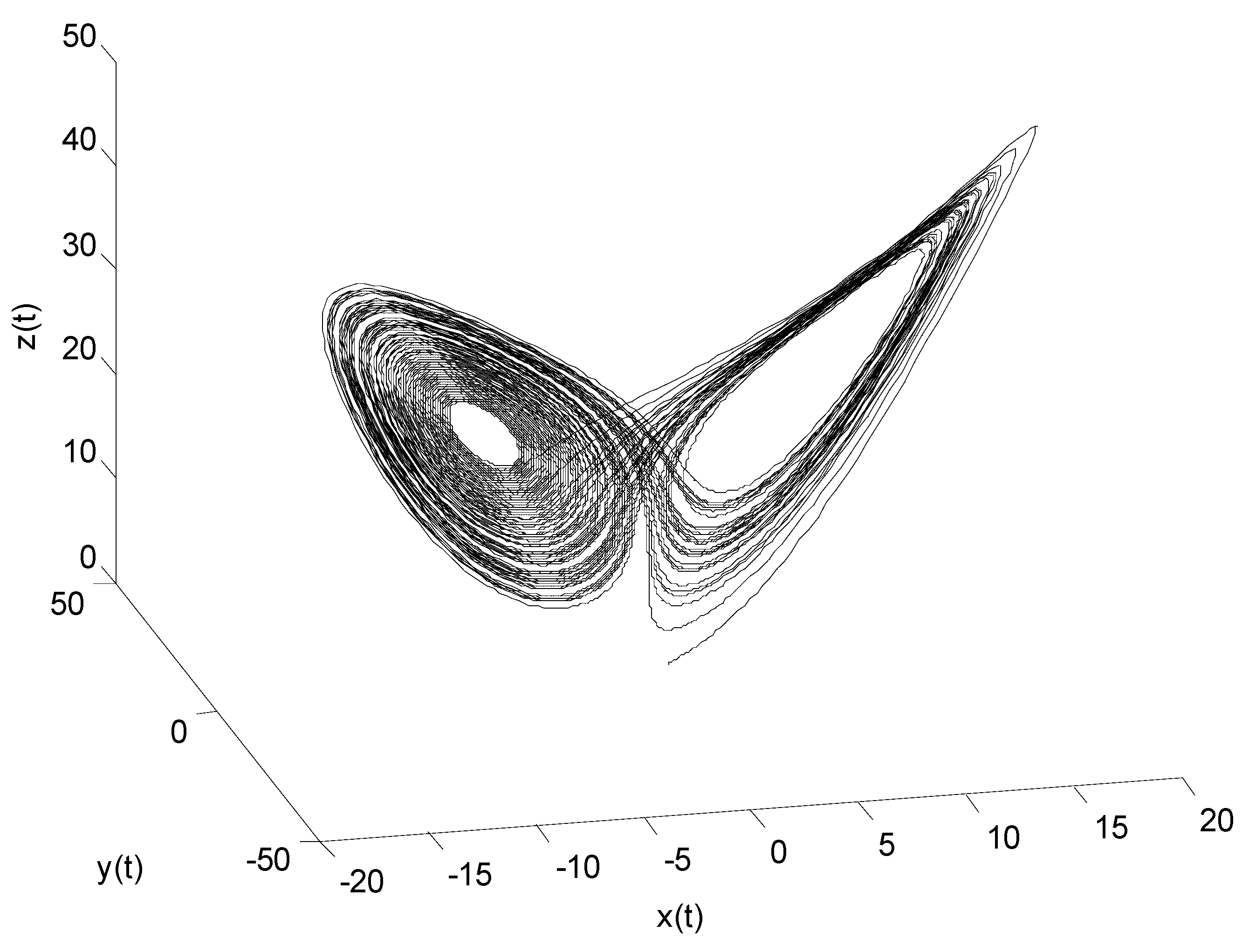
4. Illustrative Examples

In this section, we present an example to demonstrate the veracity of our findings. Consider a complex network with five nodes, where each node’s dynamical equation is represented by the following fractional-order Lorenz system:

$$\{\begin{array}{c}{D}_{*}^q{x}_1=\alpha (x_2-x_1)\hfill \\ D_{*}^q{x}_2=(\beta -x_3)x_1-x_2\hfill \\ D_{*}^q{x}_3=x_1{x}_2-\gamma x_3\hfill \end{array}$$

$$=\underset{f\left(x_i\right)}{\underbrace{\left(\begin{array}{c}0\\ -x_3{x}_1-x_2\\ x_1{x}_2\end{array}\right)}}+\underset{F\left(x_i\right)}{\underbrace{\left(\begin{array}{ccc}{x}_2-x_1& 0& 0\\ 0& x_1& 0\\ 0& 0& -x_3\end{array}\right)}}\underset{\theta }{\underbrace{\left(\begin{array}{c}\alpha \\ \beta \\ \gamma \end{array}\right)}},$$

where $x_1,x_2,x_3$ are state variables, and $\alpha =10,\beta =28,\gamma =\frac{8}{3}$. Figure 1 depicts the chaotic dynamical behavior of the fractional-order Lorenz system in which the initial states are $x(0)=\left[1,1,1\right]$ and $q_1=q_2=q_3=0.993$.

Remark 2.

In this example, we take the FOCDN in (1) and (2) with five nodes consisting of the fractional-order Lorenz system, respectively. Each node’s dynamical equation is represented by the fractional-order Lorenz system, ifthere are not any non-differentiable or vanishing points in the procedure of simulation,it satisfies Lemma2.

The controllers $u_i(t)$ can be designed by Equation (5). $\phi (t)=0.7\sin (t)\cos (t)$, $c=\overline{c}=2$, $\tau =0.1$, $H=\overline{H}=\left[\begin{array}{ccc}1& 0& 0\\ 0& 1& 0\\ 0& 0& 1\end{array}\right]$, the coupling configuration matrices $B=\overline{B}=(b_{ij})$ are chosen to be

$$B=\overline{B}=\left(\begin{array}{ccccc}-1& 0& 0& 0& 1\\ 0& -2& 1& 0& 1\\ 1& 0& -3& 1& 1\\ 0& 1& 1& -2& 0\\ 1& 0& 1& 0& -2\end{array}\right),$$

All the initial conditions are chosen as follows: $x_1(0)=[-2.5,2.5,-1.5]$, $x_2(0)=[2.5,2.5,-1.1]$, $x_3(0)=[2.7,2.9,2.1]$, $x_4(0)=[2.3,2.3,1.8]$, $x_5(0)=[-1.5,-2.5,-1.7]$, $y_1(0)=[1.5,2.7,1.9]$, $y_2(0)=[2.6,2.1,1.2]$, $y_3(0)=[-2.3,-2.3,-1]$, $y_4(0)=[-2.9,-2.3,-1.9]$, $y_5(0)=[1.9,1.9,1]$, ${\theta }_1(0)=[2,18,0.5]$, ${\theta }_2(0)=[2,18,0.9]$, ${\theta }_3(0)=[2,18,0.9]$, ${\theta }_4(0)=[2,18,0.8]$, ${\theta }_5(0)=[2,18,0.4]$, and $q_i=0.08,{\gamma }_i=30$. $\mathsf{\Lambda }=diag(2,1,2)$.

By performing simple calculations

$$\begin{array}{cc}\hfill t_1& =t_0+{\left(\frac{V(t_0)\Gamma (1+q)}{\mu }\right)}^{\frac{1}{q}}\hfill \\ & =0+{\left(\frac{48.2854\times \Gamma (1+0.993)}{31.9816}\right)}^{\frac{1}{0.993}}\hfill \\ & =1.5097,\hfill \end{array}$$

within a finite time interval, the networks in (2) can synchronize with the networks in (1). In Figure 2, the temporal evolution of the synchronization error shows that synchronization was attained at 0.53. Figure 3, Figure 4 and Figure 5 show the unknown parameter vector’s identification trajectory. We can see from Figure 3, Figure 4 and Figure 5 ${\alpha }_i(t)$, ${\beta }_i(t)$ that ${\gamma }_i(t)$ can be correctly identified in a finite time span, this further confirmed Theorem 1.

Remark 3.

FromFigure 2,Figure 3, Figure 4andFigure 5, we could see that the networks in (2) could synchronize with the networks in (1) within a finite time interval.Not only were unknown parameters of the networks estimated, but unknown bounded disturbances could also be simultaneously conquered by the proposed sufficient conditions and controllers.This further verified the effectiveness of the obtained results.

5. Conclusions

The FTPS problem of FOCDNs with uncertainties was addressed in this research. First, for FTPS of two FOCDNs with coupling delays, new controllers were developed. Second, the upper bound of the settling-time function was determined using the stability theory of fractional-order differential systems, the unknown parameters of the networks were estimated, and unknown bounded disturbances were defeated using the proposed controllers. Finally, a numerical simulation example was used to test the usefulness of the acquired conclusions. In future work, we hope to further investigate the cluster finite-time projective synchronization problem of fractional-order complex dynamical networks with different orders and disturbances.

References

1. Zhan, X.; Wu, J.; Jiang, T.; Wei, W. Optimal performance of networked control systems under the packet dropouts and channel noise. Isa Trans. 2015, 58, 214–221. [Google Scholar] [CrossRef] [PubMed]
2. Velmurugana, G.; Rakkiyappan, R.; Vembarasanb, V.; Cao, J.A.; Alsaedi, A. Dissipativity and stability analysis of fractional-order complex-valued neural networks with time delay. Neural Netw. 2017, 86, 42–53. [Google Scholar] [CrossRef] [PubMed]
3. He, Y.; Zheng, S.; Yuan, L. Dynamics of Fractional-Order Digital Manufacturing Supply Chain System and Its Control and Synchronization. Fractal Fract. 2021, 5, 128. [Google Scholar] [CrossRef]
4. Kottakkaran Sooppy, N.; Vijayakumar, V. Results concerning to approximate controllability of non-densely defined Sobolev-type Hilfer fractional neutral delay differential system. Math. Methods Appl. Sci. 2021, 44, 13615–13632. [Google Scholar]
5. Anurag, S.; Sukavanam, N.; Pandey, D.N. Controllability of Semilinear Stochastic System with Multiple Delays in Control. In Proceedings of the Third International Conference on Advances in Control and Optimization of Dynamical Systems, Kanpur, India, 13–15 March 2014. [Google Scholar]
6. Yang, X.; Song, Q.; Liu, Y.; Zhao, Z. Finite-time stability analysis of fractional-order neural networks with delay. Neurocomputing 2015, 152, 19–26. [Google Scholar] [CrossRef]
7. Kengne, R.; Tchitnga, R.; Fomethe, A.; Hammouch, Z. Neralized finite-time function projective synchronization of two fractional-order chaotic systems via a modified fractional nonsingular sliding mode surface. Commun. Numer. Anal. 2017, 2, 233–248. [Google Scholar] [CrossRef] [Green Version]
8. Feng, J.; Li, N.; Zhao, Y.; Xu, C.; Wang, J. Finite-time synchronization analysis for general complex dynamical networks with hybrid couplings and time-varying delays. Nonlinear Dyn. 2017, 88, 2723–2733. [Google Scholar] [CrossRef]
9. Anurag, S.; Sukavanam, N.; Pandey, D.N. Approximate Controllability of Semilinear Fractional Control Systems of Order α ∊ (1, 2]. In Proceedings of the Conference on Control and its Applications (CT), Paris, France, 8–10 July 2015; SIAM: Philadelphia, PA, USA, 2015; pp. 175–180. [Google Scholar]
10. Mahmoud, G.M.; Abed-Elhameed, T.M.; Ahmed, M.E. Neralization of combination- combination synchronization of chaotic n-dimensional fractional-order dynamical systems. Nonlinear Dynam. 2016, 83, 1885–1893. [Google Scholar] [CrossRef]
11. Wang, G.; Cao, J.; Lu, J. Outer synchronization between two nonidentical networks with circumstance noise. Physica A 2010, 389, 1480–1488. [Google Scholar] [CrossRef]
12. Dineshkumar, C.; Udhayakumar, R. New results concerning to approximate controllability of Hilfer fractional neutral stochastic delay integro-differential systems. Numer. Methods Partial. Differ. Equ. 2021, 37, 1072–1090. [Google Scholar] [CrossRef]
13. Dineshkumar, C.; Udhayakumar, R. Results on approximate controllability of nondensely defined fractional neutral stochastic differential systems. Numer. Methods Partial. Differ. Equ. 2020, 18. [Google Scholar] [CrossRef]
14. Wang, F.; Zheng, Z. Quasi-projectivesynchronization of fractional order chaotic Systems under input saturation. Physica A 2019, 534, 122132. [Google Scholar] [CrossRef]
15. Kong, F.; Zhu, Q. Fixed-Time Stabilization of Discontinuous Neutral Neural Networks with Proportional Delays via New Fixed-Time Stability Lemmas. IEEE Trans. Neural Netw. Learn. Syst. 2021, 1–11. [Google Scholar] [CrossRef] [PubMed]
16. Liu, M.; Wu, H.; Zhao, W. Event-triggered stochastic synchronization in finite time for delayed semi-Markovian jump neural networks with discontinuous activations. Comput. Appl. Math. 2020, 39, 118. [Google Scholar] [CrossRef]
17. Peng, X.; Wu, H.; Cao, J. Global non-fragile synchronization in finite time for fractional-order discontinuous neural networks with nonlinear growth activations. IEEE Trans. Neural Netw. Learn. Syst. 2019, 30, 2123–2137. [Google Scholar] [CrossRef]
18. Jia, Y.; Wu, H.; Cao, J. Non-fragile robust finite-time synchronization for fractional-order discontinuous complex networks with multi-weights and uncertain couolping under asynchronous switching. Appl. Math. Comput. 2020, 370, 124929. [Google Scholar]
19. Liang, S.; Wu, R.; Chen, L. Adaptive pinning synchronization in fractional-order uncertain complex dynamical networks with delay. Phys. A 2016, 444, 49–62. [Google Scholar] [CrossRef]
20. Li, H.; Cao, J.; Hu, C.; Zhang, L.; Wang, Z. Global synchronization between two fractional-order complex networks with non- delayed and delayed coupling via hybrid impulsive control. Neurocomputing 2019, 356, 31–39. [Google Scholar] [CrossRef]
21. Liu, L.; Miao, S. Outer synchronization between delayed coupling networks with different dynamics and uncertain parameters. Phys. A Stat. Mech. Appl. 2018, 512, 890–901. [Google Scholar] [CrossRef]
22. Li, R.; Wu, H.; Cao, J. Impulsive exponential synchronization of fractional-order complex dynamical networks with derivative couplings via feedback control based on discrete time state observations. Acta Math. Sci. 2022, 42, 737–754. [Google Scholar] [CrossRef]
23. Li, Y.; Kao, Y.; Wang, C.; Xia, H. Finite-time synchronization of delayed fractional-order heterogeneous complex networks. Neurocomputing 2020, 384, 368–375. [Google Scholar] [CrossRef]
24. Pratap, A.; Raja, R.; Cao, J.; Rajchakit, G.; Alsaadi, F.E. Further synchronization in finite time analysis for time-varying delayed fractional order memristive competitive neural networks with leakage delay. Neurocomputing 2018, 317, 110–126. [Google Scholar] [CrossRef]
25. Zheng, B.; Wang, S. Adaptive synchronization of fractional-order complex-valued coupled neural networks via direct error method. Neurocomputing 2022, 486, 114–122. [Google Scholar] [CrossRef]
26. Li, H.; Cao, J.; Jiang, H.; Alsaedi, A. Finite-time synchronization of fractional-order complex networks via hybrid feedback control. Neurocomputing 2018, 320, 69–75. [Google Scholar] [CrossRef]
27. Aadhithiyan, S.; Raja, R.; Zhu, Q.; Alzabut, J.; Niezabitowski, M.; Lim, C.P. Modified projective synchronization of distributive fractional order complex dynamic networks with model uncertainty via adaptive control. Chaos Solitons Fractals 2021, 147, 110853. [Google Scholar] [CrossRef]
28. Yang, Q.; Wu, H.; Cao, J. Pinning exponential cluster synchronization for fractional-order complex dynamical networks with switching topology and mode-dependent impulses. Neurocomputing 2021, 428, 182–194. [Google Scholar] [CrossRef]
29. Xiong, Y.; Wu, Z. Impulsive synchronization of fractional-order complex-variable dynamical network. Adv. Differ. Equ. 2021, 2021, 373. [Google Scholar] [CrossRef]
30. Huang, D. Synchronization-based estimation of all parameters of chaotic systems from time series. Phys. Rev. E 2004, 69, 067201. [Google Scholar] [CrossRef]
31. Wonga, W.; Li, H.; Leung, S. Robust synchronization of fractional-order complex dynamical networks with parametric uncertainties. Commun. Nonlinear Sci. Numer. Simul. 2012, 17, 4877–4890. [Google Scholar] [CrossRef]
32. Geng, L.; Xiao, R. Outer synchronization and parameter identification approach to the resilient recovery ofsupply network with uncertainty. Physica A 2017, 482, 407–421. [Google Scholar] [CrossRef]
33. Pei, J.; Fan, H.; Zhao, Y.; Feng, J. Adaptive Synchronization of Fractional-Order Nonlinearly Coupled Complex Networks With Time Delay and External Disturbances. IEEE ACCESS 2018, 6, 4653–4663. [Google Scholar] [CrossRef]
34. Chen, X.; Zhang, J.; Ma, T. Parameter estimation and topology identification of uncertain general fractional-order complex dynamical networks with time delay. IEEE/CAA J. Autom. Sinica. 2016, 3, 295–303. [Google Scholar]
35. Li, H.; Cao, J.; Jiang, H.; Alsaedi, A. Finite-time synchronization and parameter identification of Uncertain fractional-order complex networks. Physica A 2019, 533, 122027. [Google Scholar] [CrossRef]
36. Selvaraj, P.; Kwon, O.M.; Lee, S.H.; Sakthivel, R. Cluster synchronization of fractional-order complex networks via uncertainty and disturbance estimator-based modified repetitive control. J. Frankl. Inst. 2021, 358, 9951–9974. [Google Scholar] [CrossRef]
37. Du, H. Modified function projective synchronization between two fractional-order complex dynamical networks with un- known parameters and unknown bounded external disturbances. Physica A 2019, 526, 120997. [Google Scholar] [CrossRef]
38. Podlubny, I. Fractional Differential Equations; Elsevier: Amsterdam, The Netherlands, 1999. [Google Scholar]
39. Zuo, Z.; Yang, C.; Wang, Y. A unified framework of exponential synchronization for complex networks with time-varying delays. Phys. Lett. Sect. A 2010, 374, 1989–1999. [Google Scholar] [CrossRef]
40. Zhang, S.; Yu, Y.; Wang, H. Mittag-Leffler stability of fractional-order hopfield neural networks. Nonlin. Anal. Hybrid Syst. 2015, 16, 104–121. [Google Scholar] [CrossRef]
41. Alikhanov, A.A. A priori estimates for solutions of boundary value problems for fractional-order equations. Differ. Equ. 2010, 46, 660–666. [Google Scholar] [CrossRef] [Green Version]
Figure 1. Chaotic attractor of fractional-order Lorenz system.
Fractalfract 06 00298 g001
Figure 2. Time evolution of errors, e i j .
Fractalfract 06 00298 g002
Figure 3. Identification for unknown parameters, α i ( t ) .
Fractalfract 06 00298 g003
Figure 4. Identification for unknown parameters, β i ( t ) .
Fractalfract 06 00298 g004
Figure 5. Identification for unknown parameters, γ i ( t ) .
Fractalfract 06 00298 g005
Publisher’s Note: MDPI stays neutral with regard to jurisdictional claims in published maps and institutional affiliations.