Barrier Option Pricing in the Sub-Mixed Fractional Brownian Motion with Jump Environment

Abstract

This paper investigates the pricing formula for barrier options where the underlying asset is driven by the sub-mixed fractional Brownian motion with jump. By applying the corresponding $It\widehat{o}$’s formula, the B-S type PDE is derived by a self-financing strategy. Furthermore, the explicit pricing formula for barrier options is obtained through converting the PDE to the Cauchy problem. Numerical experiments are conducted to test the impact of the barrier price, the Hurst index, the jump intensity and the volatility on the value of barrier option, respectively.

1. Introduction

Barrier option is a path-dependent exotic option, whose value depends not only on the price of the underlying asset, but also on whether the price of the underlying asset touches the preset barrier price within the effective execution period of the option. For its cheaper premiums against the corresponding vanilla options, barrier options can be seen everywhere in global exchanges and over-the-counter markets. Many companies use various barrier options to hedge risks. In addition, the studies on barrier option pricing can also promote the research of many structured financial products, such as convertible bonds, bank-triggered financial products and so on. For the above reasons, the pricing of barrier options has always been a topical issue [1,2,3,4]. If the option right terminates (starts) when the underlying asset price touches the given barrier price, it is called a knock-out (in) kind; it is called a down (up) option, if the initial underlying asset price is above (below) the barrier price [5]. Therefore, single-barrier options which this paper discusses include eight types: down (up)-and-out (in) call (put) options.

In 1973, Merton [6] gave the closed solution of down-and-out European call options. Later, Reiner and Rubinstein [7] extended the pricing formulas of other European barrier options in 1991. However, these studies are under the Black–Scholes model [8] (the B-S model) which assumes the underlying asset price follows the logarithmic normal distribution. However, in recent years the self-similarity and long-range dependence has been found in the financial asset through numbers of the financial empirical studies [9,10], which is inconsistent with the B-S model. Then, Necula [11] studied the extended B-S model, where the assets price is driven by the fractional Brownian motion (fBm) instead of the Brownian motion. The fBm was first proposed by Kolmogorov [12], which exhibits self-similarity and long-range dependence. Since then, a volume of research on option-pricing models with fBm have been conducted, such as [13,14,15].

However, the fBm is neither a Markov process nor a semi-martingale, except degenerating into the Brownian motion. Although we can use Wick-self-financing strategies to analyze the fBm [16,17], Björk and Hult [18] found the application of the fBm has little economic sense, which limited its applicability in financial market. Therefore, other processes are proposed to describe the fluctuation of financial assets, such as the sub-fractional Brownian motion (sub-fBm) [19] and the sub-mixed fractional Brownian motion (sub-mixed fBm) [20].

The sub-fBm preserves most properties of the fBm, but it has the characteristics of non-stationary second-order moment increment and faster convergence [21]. Moreover, the sub-mixed fBm is a combination of the Brownian motion and the sub-fBm. When the Hurst index $H\in \left[0.75,1\right)$, the sub-mixed fBm becomes a semi martingale, which is equivalent to the Brownian motion [22]. At the same time, inspired by Merton [23] and other recent research [24,25,26], this paper introduces the jump diffusion process to describe the jump points of asset price caused by unsystematic risk factors, which is usually ignored in the pricing of barrier options. The purpose of this paper is to obtain the pricing formula of barrier options where the underlying asset is driven by the sub-mixed fBm and the compensated Poisson process.

The remainder of this paper is organized as follows: In Section 2, some necessary preliminary knowledge about the sub-fBm will be presented. In Section 3, we obtain the corresponding $It\widehat{o}$’s formula of the asset price driven by the sub-mixed fBm with jump, and give the expressions for underlying asset price. In Section 4, the Black–Scholes PDE and the closed-form solution for barrier options are obtained. In Section 5, numerical experiments are carried out to study the influences of several parameters on barrier options. Section 6 gives a summary.

2. Preliminaries

Let $\{\mathsf{\Omega },{\mathcal{F}}_t,P\}$ be a complete probability space with a filtration ${\left\{{\mathcal{F}}_t\right\}}_{t\ge 0}$ satisfying the usual conditions.

Definition 1. 

The sub-mixed fBm ${\xi }_t^H={\left\{{\xi }_t^H(\alpha ,\beta )\right\}}_{t\ge 0}$ is a linear combination of the Brownian motion ${\left\{B_t\right\}}_{t\ge 0}$ and the sub-fBm ${\left\{B_t^H\right\}}_{t\ge 0}$, which can be expressed as:

$${\xi }_t^H(\alpha ,\beta )=\alpha B_t+\beta B_t^H,\forall t\ge 0,$$

where H is the Hurst index, $\alpha and\beta$ are positive constants, ${\left\{B_t\right\}}_{t\ge 0}$ and ${\left\{B_t^H\right\}}_{t\ge 0}$ are independent of each other.

Lemma 1. 

The sub-mixed fBm ${\xi }_t^H={\left\{{\xi }_t^H(\alpha ,\beta )\right\}}_{t\ge 0}$ has the following properties [20]:

1. 

${\left\{{\xi }_t^H(\alpha ,\beta )\right\}}_{t\ge 0}$ is a central Gaussian process.

2. 

When $t=0$, ${\xi }_0^H(\alpha ,\beta )=\alpha B_0+\beta B_0^H=0.$

3. 

$\forall t,s\ge 0,$ the covariance of ${\xi }_t^H(\alpha ,\beta )$ and ${\xi }_s^H(\alpha ,\beta )$ is

$$Cov\left({\xi }_t^H(\alpha ,\beta ),{\xi }_s^H(\alpha ,\beta )\right)={\alpha }^2(t\wedge s)+\frac{{\beta }^2}{2}\left(t^{2H}+s^{2H}-{|t-s|}^{2H}\right),$$

where $t\wedge s=\frac{1}{2}(t+s-|t-s\left|\right).$

4. 

$\forall t\ge 0$, $E\left({\left({\xi }_t^H(\alpha ,\beta )\right)}^2\right)={\alpha }^{2}t+{\beta }^2\left(2-2^{2H-1}\right)t^{2H}$.

3. Asset Pricing Model

In this paper, we adopt the classical financial stochastic analysis theory and make some extensions for the B-S model. Furthermore, the following assumptions are hold:

• There are two kinds of assets in the financial market: risk-free assets (bonds) and risky assets (stocks).
• The stock price $S_t$ is driven by the sub-mixed fBm with jump:

  $$\begin{array}{cc}\hfill d{S}_t& =(\mu -q)S_{t}dt+S_{t}d{\xi }_t^H(\alpha ,\beta )+\gamma S_{t}d{J}_t\hfill \\ \hfill & =(\mu -q)S_{t}dt+\alpha S_{t}d{B}_t+\beta S_{t}d{B}_t^H+\gamma S_{t}d{J}_t,\hfill \end{array}$$

  (1)

  where $\mu$ is the instantaneous expected return rate of the stock; q is the stock dividend rate; $\alpha ,\beta$ and $\gamma$ represent the volatility of stock price; ${\left\{J_t\right\}}_{t\ge 0}$ is a compensated Poisson process with intensity $\lambda$. ${\left\{B_t\right\}}_{t\ge 0}$, ${\left\{B_t^H\right\}}_{t\ge 0}$ and ${\left\{J_t\right\}}_{t\ge 0}$ are independent of each other.
• The return of risk-free assets in time period t is

  $$d{M}_t=r{M}_{t}dt,$$

  (2)

  where constant r is the risk-free interest rate.
• All assets can be traded freely and continuously without transaction costs and taxes.
• There is no arbitrage opportunity in the market.
• Short selling is not limited.
• The option can be exercised only at the maturity time.

Remark 1. 

It is worth mentioning that there are some limitations when the B-S type model is applied, which are detailed in references [27,28,29,30]. In this paper, we focus on the classical setting of B-S model and will not elaborate too much here. If possible, further research can be carried out in the future.

Theorem 1. 

Assume that $Y_t={\xi }_t^H(\alpha ,\beta )+\gamma J_t$ with the initial value zero, and $f\left(t,Y_t\right)$ is second-order differentiable. Then, the $It\widehat{o}$’s formula of the sub-mixed fBm with jump can be expressed as follows:

$$\begin{array}{cc}\hfill f\left(t,Y_t\right)=& f(0,0)+{\int }_0^t\left[\frac{\partial f}{\partial s}-\lambda \gamma \frac{\partial f}{\partial Y}\right]ds+{\int }_0^t\left[\frac{{\alpha }^2}{2}+\left(2-2^{2H-1}\right)H{\beta }^2{s}^{2H-1}\right]\frac{{\partial }^{2}f}{\partial Y^2}ds\hfill \\ & +\alpha {\int }_0^t\frac{\partial f}{\partial Y}d{B}_s+\beta {\int }_0^t\frac{\partial f}{\partial Y}d{B}_s^H+\sum _{s\le t}\left[f\left(s,Y_s\right)-f\left(s-,Y_{s-}\right)\right]\hfill \\ \hfill =& f(0,0)+{\int }_0^t\left\{\frac{\partial f}{\partial s}+\left[\frac{{\alpha }^2}{2}+\frac{\lambda {\gamma }^2}{2}+\left(2-2^{2H-1}\right)H{\beta }^2{s}^{2H-1}\right]\frac{{\partial }^{2}f}{\partial Y^2}\right\}ds\hfill \\ & +\alpha {\int }_0^t\frac{\partial f}{\partial Y}d{B}_s+\beta {\int }_0^t\frac{\partial f}{\partial Y}d{B}_s^H+\gamma {\int }_0^t\frac{\partial f}{\partial Y}d{J}_s.\hfill \end{array}$$

Proof. 

According to the sub-mixed fBm $It\widehat{o}$’s formula [20] and the jump process analysis method [31], we have

$$\begin{array}{cc}f\left(t,Y_t\right)\hfill & =f(0,0)+{\int }_0^t\frac{\partial f}{\partial s}ds+{\int }_0^t\frac{\partial f}{\partial S}d{Y}_s^c+\frac{1}{2}{\int }_0^t\frac{{\partial }^{2}f}{\partial S^2}{\left(d{Y}_s^c\right)}^2+\sum _{s\le t}\left[f\left(s,Y_s\right)-f\left(s-,Y_{s-}\right)\right]\hfill \\ & =f(0,0)+{\int }_0^t\left[\frac{\partial f}{\partial s}-\lambda \gamma \frac{\partial f}{\partial Y}\right]ds+{\int }_0^t\left[\frac{{\alpha }^2}{2}+\left(2-2^{2H-1}\right)H{\beta }^2{s}^{2H-1}\right]\frac{{\partial }^{2}f}{\partial Y^2}ds\hfill \\ & +\alpha {\int }_0^t\frac{\partial f}{\partial Y}d{B}_s+\beta {\int }_0^t\frac{\partial f}{\partial Y}d{B}_s^H+\sum _{s\le t}\left[f\left(s,Y_s\right)-f\left(s-,Y_{s-}\right)\right].\hfill \end{array}$$

(3)

The following identities are used:

$$d{Y}_t^c=\alpha d{B}_t+\beta d{B}_t^H-\lambda \gamma dt,$$

$${\left(d{Y}_t^c\right)}^2=\left[{\alpha }^2+2\left(2-2^{2H-1}\right)H{\beta }^2{t}^{2H-1}\right]dt$$

and $Y_t^c=\alpha B_t+\beta B_t^H-\lambda \gamma t$ is the continuous part of $Y_t$.

If $g\left(x\right)$ is second order differentiable. Given that Poisson process ${\left\{N_t\right\}}_{t\ge 0}$ with intensity λ has the second-order moment increments $<d{N}_t,d{N}_t>=\lambda dt$, by generalized $It\widehat{o}$’s formula we obtain

$$\sum _{s\le t}\left[g\left(N_s\right)-g\left(N_{s-}\right)\right]={\int }_0^t\frac{\partial g}{\partial N}d{N}_s+\frac{\lambda }{2}{\int }_0^t\frac{{\partial }^{2}g}{\partial N^2}ds.$$

Combining $Y_t={\xi }_t^H(\alpha ,\beta )+\gamma J_t=\alpha B_t+\beta B_t^H+\gamma N_t-\lambda \gamma t$, we arrive at

$$\sum _{s\le t}\left[f\left(s,Y_s\right)-f\left(s,Y_{s-}\right)\right]=\gamma {\int }_0^t\frac{\partial f}{\partial Y}d{N}_s+\frac{\lambda {\gamma }^2}{2}{\int }_0^t\frac{{\partial }^{2}f}{\partial Y^2}ds.$$

(4)

Substitute (4) back to (3), which yields

$$\begin{array}{cc}\hfill f\left(t,Y_t\right)=& f(0,0)+{\int }_0^t\left\{\frac{\partial f}{\partial s}+\left[\frac{{\alpha }^2}{2}+\frac{\lambda {\gamma }^2}{2}+\left(2-2^{2H-1}\right)H{\beta }^2{s}^{2H-1}\right]\frac{{\partial }^{2}f}{\partial Y^2}\right\}ds\hfill \\ & +\alpha {\int }_0^t\frac{\partial f}{\partial Y}d{B}_s+\beta {\int }_0^t\frac{\partial f}{\partial Y}d{B}_s^H+\gamma {\int }_0^t\frac{\partial f}{\partial Y}d{J}_s.\hfill \end{array}$$

□

Theorem 2. 

The stock price satisfying (1) has the following explicit solution:

$$S_t=S_{0}exp\left\{(\mu -q)t-\left[\left(\frac{{\alpha }^2}{2}+\frac{\lambda {\gamma }^2}{2}\right)t+\left(1-2^{2H-2}\right){\beta }^2{t}^{2H}\right]+\alpha B_t+\beta B_t^H+\gamma J_t\right\}.$$

Proof. 

Let $f\left(t,Y_t\right)=S_{0}exp\left\{(\mu -q)t-\left[\left(\frac{{\alpha }^2}{2}+\frac{\lambda {\gamma }^2}{2}\right)t+\left(1-2^{2H-2}\right){\beta }^2{t}^{2H}\right]+Y_t\right\}$.

An application of Theorem 1 yields

$$\begin{array}{cc}\hfill df\left(t,Y_t\right)& =\left\{\frac{\partial f}{\partial t}+\left[\frac{{\alpha }^2}{2}+\frac{\lambda {\gamma }^2}{2}+\left(2-2^{2H-1}\right)H{\beta }^2{t}^{2H-1}\right]\frac{{\partial }^{2}f}{\partial Y^2}\right\}dt+\frac{\partial f}{\partial Y}d{Y}_t.\hfill \\ \hfill & =(\mu -q)f\left(t,Y_t\right)dt+f\left(t,Y_t\right)d{Y}_t\hfill \\ \hfill & =(\mu -q)f\left(t,Y_t\right)dt+f\left(t,Y_t\right)d{\xi }_t^H(\alpha ,\beta )+\gamma f\left(t,Y_t\right)d{J}_t,\hfill \end{array}$$

(5)

where

$$\begin{array}{cc}\hfill \frac{\partial f}{\partial t}& =\left\{(\mu -q)-\left[\left(\frac{{\alpha }^2}{2}+\frac{\lambda {\gamma }^2}{2}\right)+\left(2-2^{2H-1}\right)H{\beta }^2{t}^{2H-1}\right]\right\}f\left(t,Y_t\right),\hfill \\ \hfill \frac{\partial f}{\partial Y}& =f\left(t,Y_t\right)and\frac{{\partial }^{2}f}{\partial Y^2}=f\left(t,Y_t\right).\hfill \end{array}$$

Comparing (1) and (5), we can deduce $d{S}_t=df(t,Y_t)$, where the values are the same $f(0,Y_0)=S_0$. Therefore,

$$\begin{array}{cc}\hfill S_t& =f\left(t,Y_t\right)\hfill \\ & =S_{0}exp\left\{(\mu -q)t-\left[\left(\frac{{\alpha }^2}{2}+\frac{\lambda {\gamma }^2}{2}\right)t+\left(1-2^{2H-2}\right){\beta }^2{t}^{2H}\right]+\alpha B_t+\beta B_t^H+\gamma J_t\right\}.\hfill \end{array}$$

□

4. Pricing Formula for Barrier Options

With the explicit solution of the stock price $S_t$ in hand, in this section the pricing formula for battier options can be derived.

Theorem 3. 

Assuming that the underlying asset price $S_t$ follows (1), then the value of contingent claims $V_t=V(t,S_t)$ satisfies the following PDE:

$$\frac{\partial V}{\partial t}+(r-q)S_t\frac{\partial V}{\partial S}+\left[\frac{{\alpha }^2}{2}+\frac{\lambda {\gamma }^2}{2}+\left(2-2^{2H-1}\right)H{\beta }^2{t}^{2H-1}\right]S_t^2\frac{{\partial }^{2}V}{\partial S^2}-r{V}_t=0.$$

Proof. 

Using the self-financing strategy ${\theta }_t=\left({\theta }_t^1,{\theta }_t^2\right)$, we hold a number of ${\theta }_t^1$ bonds and ${\theta }_t^2$ stocks to build the wealth process, whose value at time t is

$$V_t={\theta }_t^1{M}_t+{\theta }_t^2{S}_t.$$

(6)

Combining (1) and (2), we obtain

$$\begin{array}{cc}\hfill d{V}_t& ={\theta }_t^{1}d{M}_t+{\theta }_t^{2}d{S}_t+{\theta }_t^{2}q{S}_{t}dt\hfill \\ \hfill & =\left(r{\theta }_t^1{M}_t+\mu {\theta }_t^2{S}_t\right)dt+{\theta }_t^2{S}_t\left(\alpha d{B}_t+\beta d{B}_t^H+\gamma d{J}_t\right).\hfill \end{array}$$

(7)

At the same time, by applying Theorems 1 and 2, we have

$$\begin{array}{cc}\hfill d{V}_t=& \frac{\partial V}{\partial t}dt+\frac{\partial V}{\partial S}d{S}_t+\frac{1}{2}\frac{{\partial }^{2}V}{\partial S^2}{\left(d{S}_t\right)}^2\hfill \\ \hfill =& \left\{\frac{\partial V}{\partial t}+(\mu -q)S_t\frac{\partial V}{\partial S}+\left[\frac{{\alpha }^2}{2}+\frac{\lambda {\gamma }^2}{2}+\left(2-2^{2H-1}\right)H{\beta }^2{t}^{2H-1}\right]S_t^2\frac{{\partial }^{2}V}{\partial S^2}\right\}dt\hfill \\ \hfill & +S_t\frac{\partial V}{\partial S}\left(\alpha d{B}_t+\beta d{B}_t^H+\gamma d{J}_t\right),\hfill \end{array}$$

(8)

where ${\left(d{S}_t\right)}^2=S_t^2\left[\left({\alpha }^2+\lambda {\gamma }^2\right)+2\left(2-2^{2H-1}\right)H{\beta }^2{t}^{2H-1}\right]dt$.

Comparing (7) and (8), ${\theta }_t^1$ and ${\theta }_t^2$ are given

$$\left\{\begin{array}{c}{\theta }_t^1={\left(r{M}_t\right)}^{-1}\left\{{\displaystyle \frac{\partial V}{\partial t}}-q{S}_t{\displaystyle \frac{\partial V}{\partial S}}+\left[{\displaystyle \frac{{\alpha }^2}{2}}+{\displaystyle \frac{\lambda {\gamma }^2}{2}}+\left(2-2^{2H-1}\right)H{\beta }^2{t}^{2H-1}\right]S_t^2{\displaystyle \frac{{\partial }^{2}V}{\partial S^2}}\right\},\hfill \\ {\theta }_t^2={\displaystyle \frac{\partial V}{\partial S}}.\hfill \end{array}\right.$$

(9)

From (6), we obtain

$${\theta }_t^1=\frac{V_t-{\theta }_t^2{S}_t}{M_t}.$$

(10)

Combining (9) and (10), Theorem 3 is proved. □

Theorem 4. 

Suppose that the underlying asset price $S_t$ satisfies (1), then at time t the value of the down-and-out call option $C_{do}\left(t,S_t\right)$ with the fixed strike price K, the fixed barrier L and the maturity time T is given

$$\begin{array}{cc}\hfill C_{do}\left(t,S_t\right)=& S_t{e}^{-q(T-t)}N\left(d_1\right)-K{e}^{-r(T-t)}N\left(d_2\right)\hfill \\ & -{\left(\frac{S_t}{L}\right)}^{\kappa \left(t\right)}\left[\frac{L^2}{S_t}{e}^{-q(T-t)}N\left(d_3\right)-K{e}^{-r(T-t)}N\left(d_4\right)\right].\hfill \end{array}$$

The following identities are used: $N\left(x\right)=\frac{1}{\sqrt{2\pi }}{\int }_{-\infty }^x{e}^{-\frac{t^2}{2}}dt$, which denotes the cumulative probability of standard normal distribution;

$$\begin{array}{c}{d}_1={\displaystyle \frac{ln\frac{S_t}{K}+\left(r-q+\frac{{\alpha }^2}{2}+\frac{\lambda {\gamma }^2}{2}\right)(T-t)+\left(1-2^{2H-2}\right){\beta }^2\left(T^{2H}-t^{2H}\right)}{\sqrt{\left({\alpha }^2+\lambda {\gamma }^2\right)(T-t)+\left(2-2^{2H-1}\right){\beta }^2\left(T^{2H}-t^{2H}\right)}}};\hfill \\ d_2=d_1-\sqrt{\left({\alpha }^2+\lambda {\gamma }^2\right)(T-t)+\left(2-2^{2H-1}\right){\beta }^2\left(T^{2H}-t^{2H}\right)};\hfill \\ d_3={\displaystyle \frac{ln\frac{L^2}{K{S}_t}+\left(r-q+\frac{{\alpha }^2}{2}+\frac{\lambda {\gamma }^2}{2}\right)(T-t)+\left(1-2^{2H-2}\right){\beta }^2\left(T^{2H}-t^{2H}\right)}{\sqrt{\left({\alpha }^2+\lambda {\gamma }^2\right)(T-t)+\left(2-2^{2H-1}\right){\beta }^2\left(T^{2H}-t^{2H}\right)}}};\hfill \\ d_4=d_3-\sqrt{\left({\alpha }^2+\lambda {\gamma }^2\right)(T-t)+\left(2-2^{2H-1}\right){\beta }^2\left(T^{2H}-t^{2H}\right)};\hfill \\ \kappa \left(t\right)=1-{\displaystyle \frac{2(r-q)(T-t)}{\left({\alpha }^2+\lambda {\gamma }^2\right)(T-t)+\left(2-2^{2H-1}\right){\beta }^2\left(T^{2H}-t^{2H}\right)}}.\hfill \end{array}$$

Proof. 

Let $V_t(t,S_t)=C_{do}(t,S_t)=C_{do}$. Then according to Theorem 3, the value of the down-and-out call option $C_{do}\left(t,S_t\right)$ is given by

$${\displaystyle \frac{\partial C_{do}}{\partial t}}+(r-q)S_t{\displaystyle \frac{\partial C_{do}}{\partial S}}+\left[{\displaystyle \frac{{\alpha }^2}{2}}+{\displaystyle \frac{\lambda {\gamma }^2}{2}}+\left(2-2^{2H-1}\right)H{\beta }^2{t}^{2H-1}\right]S_t^2{\displaystyle \frac{{\partial }^2{C}_{do}}{\partial S^2}}-r{C}_{do}=0,$$

with the initial condition $C_{do}\left(T,S_T\right)={\left(S_T-K\right)}^{+},L<S_t<+\infty ,$ and the boundary condition $C_{do}(t,L)=0,0\le t\le T.$

Let

$$x=ln\frac{S_t}{L},C_{do}\left(t,S_t\right) = L\widehat{C}(t,x).$$

(11)

Then,

$${\displaystyle \frac{\partial C_{do}}{\partial t}}=L{\displaystyle \frac{\partial \widehat{C}}{\partial t}},{\displaystyle \frac{\partial C_{do}}{\partial S}}=L{\displaystyle \frac{\partial \widehat{C}}{\partial x}}{\displaystyle \frac{\partial x}{\partial S}}={\displaystyle \frac{L}{S_t}}{\displaystyle \frac{\partial \widehat{C}}{\partial x}}and{\displaystyle \frac{{\partial }^2{C}_{do}}{\partial S^2}}={\displaystyle \frac{L}{S_t^2}}\left[{\displaystyle \frac{{\partial }^2\widehat{C}}{\partial x^2}}-{\displaystyle \frac{\partial \widehat{C}}{\partial x}}\right].$$

Therefore, we can deduce that

$${\displaystyle \frac{\partial \widehat{C}}{\partial t}}+(r-q){\displaystyle \frac{\partial \widehat{C}}{\partial x}}+\left[{\displaystyle \frac{{\alpha }^2}{2}}+{\displaystyle \frac{\lambda {\gamma }^2}{2}}+\left(2-2^{2H-1}\right)H{\beta }^2{t}^{2H-1}\right]\left({\displaystyle \frac{{\partial }^2\widehat{C}}{\partial x^2}}-{\displaystyle \frac{\partial \widehat{C}}{\partial x}}\right)-r\widehat{C}=0,$$

with the initial condition $\widehat{C}\left(T,ln{\displaystyle \frac{S_T}{L}}\right)={\left(e^x-{\displaystyle \frac{K}{L}}\right)}^{+},0<x<+\infty ,$ and the boundary condition $\widehat{C}(0,t)=0,0\le t\le T$.

Next, let

$$\omega (\tau ,\eta )=\widehat{C}(x,t)e^{b\left(t\right)},\tau =c\left(t\right),\eta =x+a\left(t\right),$$

(12)

where $a\left(t\right),b\left(t\right)$ and $c\left(t\right)$ are undetermined functions about t, which are first order differentiable. Then, we derive

$${\displaystyle \frac{\partial \widehat{C}}{\partial t}}=e^{-b\left(t\right)}\left[a^{\prime }\left(t\right){\displaystyle \frac{\partial \omega }{\partial \eta }}+c^{\prime }\left(t\right){\displaystyle \frac{\partial \omega }{\partial \tau }}-b^{\prime }\left(t\right)\omega \right],{\displaystyle \frac{\partial \widehat{C}}{\partial x}}=e^{-b\left(t\right)}{\displaystyle \frac{\partial \omega }{\partial \eta }},{\displaystyle \frac{{\partial }^2\widehat{C}}{\partial x^2}}=e^{-b\left(t\right)}{\displaystyle \frac{{\partial }^2\omega }{\partial {\eta }^2}}$$

and

$$c^{\prime }\left(t\right)\frac{\partial \omega }{\partial \tau }+\sigma \left(t\right)\frac{{\partial }^2\omega }{\partial {\eta }^2}+\left[r-q+a^{\prime }\left(t\right)-\sigma \left(t\right)\right]\frac{\partial \widehat{C}}{\partial x}-\left[r+b^{\prime }\left(t\right)\right]\omega =0,$$

(13)

where $\sigma \left(t\right)={\displaystyle \frac{{\alpha }^2}{2}}+{\displaystyle \frac{\lambda {\gamma }^2}{2}}+(2-2^{2H-1})H{\beta }^2{t}^{2H-1}.$

In order for the solution, let

$$\left\{\begin{array}{c}{c}^{\prime }\left(t\right)+\sigma \left(t\right)=0,\hfill \\ r-q+a^{\prime }\left(t\right)-\sigma \left(t\right)=0,\hfill \\ r+b^{\prime }\left(t\right)=0,\hfill \\ a\left(T\right)=b\left(T\right)=c\left(T\right)=0,\hfill \end{array}\right.$$

(14)

to convert (13) into the heat equation.

From (14), $a\left(t\right),b\left(t\right)$ and $c\left(t\right)$ are given

$$\left\{\begin{array}{c}{\displaystyle a\left(t\right)={\int }_t^{T}r-q-\sigma \left(s\right)ds=\left(r-q-{\displaystyle \frac{{\alpha }^2}{2}}-{\displaystyle \frac{\lambda {\gamma }^2}{2}}\right)(T-t)-\left(1-2^{2H-2}\right){\beta }^2\left(T^{2H}-t^{2H}\right),}\hfill \\ {\displaystyle b\left(t\right)={\int }_t^{T}rds=r(T-t),}\hfill \\ c\left(t\right)=\left({\displaystyle \frac{{\alpha }^2}{2}}+{\displaystyle \frac{\lambda {\gamma }^2}{2}}\right)(T-t)+\left(1-2^{2H-2}\right){\beta }^2\left(T^{2H}-t^{2H}\right).\hfill \end{array}\right.$$

(15)

Substitute (15) into (13), then the value of the down-and-out call option $C_{do}\left(t,S_t\right)$ is given by

$${\displaystyle \frac{\partial \omega }{\partial \tau }}={\displaystyle \frac{{\partial }^2\omega }{\partial {\eta }^2}},$$

(16)

with the initial condition $\omega (0,\eta )={(e^{\eta }-K)}^{+},0<\eta <+\infty ,$ and the boundary condition $\omega (\tau ,a(t\left)\right)=0,0\le t\le T.$

Notice that if we just consider PDE with its initial condition, the solution can be obtained by the Poisson formula

$$\omega (\tau ,\eta )=\frac{1}{2\sqrt{\pi \tau }}{\int }_{-\infty }^{+\infty }\phi \left(z\right)e^{-\frac{{(\eta -z)}^2}{4\tau }}dz.$$

(17)

To deal with the boundary condition, let $G\left(z\right)=\phi \left(z\right)e^{-\frac{{[a\left(t\right)-z]}^2}{4\tau }}$ when $z>0$. Then we extend $G\left(z\right)$ to become an odd function in the whole real number field

$$G\left(z\right)=\left\{\begin{array}{cc}\phi \left(z\right)e^{-\frac{{[a\left(t\right)-z]}^2}{4\tau }},\hfill & z>0,\hfill \\ -\phi (-z)e^{\frac{{[a\left(t\right)+z]}^2}{4\tau }},\hfill & z\le 0.\hfill \end{array}\right.$$

Comparing the above equation and the original initial condition in (16), we obtain extended initial condition which contains the boundary condition

$$\phi \left(z\right)=\left\{\begin{array}{cc}{\left(e^z-\frac{K}{L}\right)}^{+},\hfill & z>0,\hfill \\ -{\left(e^{-z}-\frac{K}{L}\right)}^{+}{e}^{-\frac{a\left(t\right)z}{\tau }},\hfill & z\le 0.\hfill \end{array}\right.$$

Therefore, (16) will be transformed into a Cauchy problem

$${\displaystyle \frac{\partial \omega }{\partial \tau }}={\displaystyle \frac{{\partial }^2\omega }{\partial {\eta }^2}},$$

(18)

with the initial condition $\omega (0,\eta )=\phi \left(\eta \right),-\infty <\eta <+\infty .$

According to (17),

$$\begin{array}{cc}\hfill \omega (\tau ,\eta )=& \frac{1}{2\sqrt{\pi \tau }}{\int }_{-\infty }^{+\infty }\phi \left(z\right)e^{-\frac{{(\eta -z)}^2}{4\tau }}dz\hfill \\ \hfill =& \frac{1}{2\sqrt{\pi \tau }}{\int }_{ln\frac{K}{L}}^{+\infty }\left(e^z-\frac{K}{L}\right)e^{-\frac{{(\eta -z)}^2}{4\tau }}dz-\frac{1}{2\sqrt{\pi \tau }}{\int }_{-\infty }^{-ln\frac{K}{L}}\left(e^{-z}-\frac{K}{L}\right)e^{-\frac{{(\eta -z)}^2+4a\left(t\right)z}{4\tau }}dz\hfill \\ \hfill =& \frac{1}{2\sqrt{\pi \tau }}{\int }_{ln\frac{K}{L}}^{+\infty }{e}^{z-\frac{{(\eta -z)}^2}{4\tau }}dz-\frac{1}{2\sqrt{\pi \tau }}\frac{K}{L}{\int }_{ln\frac{K}{L}}^{+\infty }{e}^{-\frac{{(\eta -z)}^2}{4\tau }}dz-\frac{1}{2\sqrt{\pi \tau }}{\int }_{ln\frac{K}{L}}^{+\infty }{e}^{z-\frac{{(\eta +z)}^2-4a\left(t\right)z}{4\tau }}dz\hfill \\ & +\frac{1}{2\sqrt{\pi \tau }}\frac{K}{L}{\int }_{ln\frac{K}{L}}^{+\infty }{e}^{\frac{{(\eta +z)}^2-4a\left(t\right)z}{4\tau }}dz\hfill \\ \hfill =& I_1+I_2+I_3+I_4.\hfill \end{array}$$

For convenience, define $N\left(x\right)$ as follows: $N\left(x\right)=\frac{1}{\sqrt{2\pi }}{\int }_{-\infty }^x{e}^{-\frac{t^2}{2}}dt$, which represents the cumulative probability of standard normal distribution.

For $I_1$,

$${\displaystyle I_1={\displaystyle \frac{1}{2\sqrt{\pi \tau }}}{\int }_{ln\frac{K}{L}}^{+\infty }{e}^{z-\frac{{(\eta -z)}^2}{4\tau }}dz=e^{\tau +\eta }{\displaystyle \frac{1}{2\sqrt{\pi \tau }}}{\int }_{ln\frac{K}{L}}^{+\infty }{e}^{-\frac{{(z-\eta -2\tau )}^2}{4\tau }}dz.}$$

Let $t=\frac{z-\eta -2\tau }{\sqrt{2\tau }},$ then

$$I_1=e^{\tau +\eta }\frac{1}{\sqrt{2\pi }}{\int }_{\frac{ln\frac{K}{L}-\eta -2\tau }{\sqrt{2\tau }}}^{+\infty }{e}^{-\frac{t^2}{2}}dt=e^{\tau +\eta }N\left(d_1\right),$$

where $d_1={\displaystyle \frac{\eta +2\tau -ln\frac{K}{L}}{\sqrt{2\tau }}}.$

Similarly, let $t=\frac{z-\eta }{\sqrt{2\tau }}$ and obtain

$${\displaystyle I_2=-{\displaystyle \frac{1}{2\sqrt{\pi \tau }}}{\displaystyle \frac{K}{L}}{\int }_{ln\frac{K}{L}}^{+\infty }{e}^{-\frac{{(\eta -z)}^2}{4\tau }}dz=-{\displaystyle \frac{K}{L}}\frac{1}{\sqrt{2\pi }}{\int }_{\frac{ln\frac{K}{L}-\eta }{\sqrt{2\tau }}}^{+\infty }{e}^{-\frac{t^2}{2}}dt=-{\displaystyle \frac{K}{L}}N\left(d_2\right),}$$

where $d_2={\displaystyle \frac{\eta -ln\frac{K}{L}}{\sqrt{2\tau }}}=d_1-\sqrt{2\tau }$.

For $I_3$,

$$I_3=-\frac{1}{2\sqrt{\pi \tau }}{\int }_{ln\frac{K}{L}}^{+\infty }{e}^{z-\frac{{(\eta +z)}^2-4a\left(t\right)z}{4\tau }}dz=-e^{\frac{[\tau +a(t\left)\right][\tau +a(t)-\eta ]}{\tau }}\frac{1}{2\sqrt{\pi \tau }}{\int }_{ln\frac{K}{L}}^{+\infty }{e}^{-\frac{{[z+\eta -2a\left(t\right)-2\tau ]}^2}{4\tau }}dz.$$

Let $t=\frac{z+\eta -2a\left(t\right)-2\tau }{\sqrt{2\tau }}$, then

$$I_3=-e^{\frac{[\tau +a(t\left)\right][\tau +a(t)-\eta ]}{\tau }}\frac{1}{\sqrt{2\pi }}{\int }_{\frac{ln\frac{K}{L}+\eta -2a\left(t\right)-2\tau }{\sqrt{2\tau }}}^{+\infty }{e}^{-\frac{t^2}{2}}dt=-e^{\frac{[\tau +a(t\left)\right][\tau +a(t)-\eta ]}{\tau }}N\left(d_3\right),$$

where $d_3={\displaystyle \frac{2a\left(t\right)+2\tau -\eta -ln\frac{K}{L}}{\sqrt{2\tau }}}.$

For $I_4$, let $t=\frac{z+\eta -2a\left(t\right)}{\sqrt{2\tau }}$, we derive

$$\begin{array}{cc}\hfill I_4& =\frac{1}{2\sqrt{\pi \tau }}\frac{K}{L}{\int }_{ln\frac{K}{L}}^{+\infty }{e}^{-\frac{{(\eta +z)}^2-4a\left(t\right)z}{4\tau }}dz=\frac{K}{L}{e}^{\frac{a\left(t\right)\left[a\right(t)-\eta ]}{\tau }}\frac{1}{2\sqrt{\pi \tau }}{\int }_{ln\frac{K}{L}}^{+\infty }{e}^{-\frac{{[z+\eta -2a\left(t\right)]}^2}{4\tau }}dz\hfill \\ & =e^{\frac{a\left(t\right)\left[a\right(t)-\eta ]}{\tau }}\frac{1}{\sqrt{2\pi }}{\int }_{\frac{ln\frac{K}{L}+\eta -2a\left(t\right)}{\sqrt{2\tau }}}^{+\infty }{\displaystyle \frac{K}{L}}{e}^{-\frac{t^2}{2}}dt=\frac{K}{L}{e}^{\frac{a\left(t\right)\left[a\right(t)-\eta ]}{\tau }}N\left(d_4\right),\hfill \end{array}$$

where, $d_4={\displaystyle \frac{2a\left(t\right)-\eta -ln\frac{K}{L}}{\sqrt{2\tau }}}=d_3-\sqrt{2\tau }.$

Substitute (11) and (12) in them, then

$$\begin{array}{cc}\hfill I_1=& \frac{S_t}{L}{e}^{(r-q)(T-t)}N\left(d_1\right);\hfill \\ \hfill I_2=& -\frac{K}{L}N\left(d_2\right);\hfill \\ \hfill I_3=& -e^{\frac{(r-q)(T-t)\left(\tau -ln\frac{S_t}{L}\right)}{\tau }}N\left(d_3\right)=-e^{(r-q)(T-t)+\left[1-\frac{(r-q)(T-t)}{\tau }\right]ln\frac{S_t}{L}-ln\frac{S_t}{L}}N\left(d_3\right)\hfill \\ \hfill =& -e^{(r-q)(T-t)}{\left(\frac{S_t}{L}\right)}^{1-\frac{(r-q)(T-t)}{\tau }}\frac{L}{S_t}N\left(d_3\right);\hfill \\ \hfill I_4=& \frac{K}{L}{e}^{\frac{[\tau -(r-q)(T-t)]ln\frac{S_t}{L}}{\tau }}N\left(d_4\right)=\frac{K}{L}{\left(\frac{S_t}{L}\right)}^{1-\frac{(r-q)(T-t)}{\tau }}N\left(d_4\right).\hfill \end{array}$$

By combining $I_1,I_2,I_3,and{I}_4$, we have

$$\begin{array}{cc}\hfill C_{do}\left(t,S_t\right)=& L\widehat{C}(t,x)=L{e}^{-r(T-t)}\omega (\tau ,\eta )=L{e}^{-r(T-t)}(I_1+I_2+I_3+I_4)\hfill \\ \hfill =& S_t{e}^{-q(T-t)}N\left(d_1\right)-K{e}^{-r(T-t)}N\left(d_2\right)\hfill \\ & -{\left(\frac{S_t}{L}\right)}^{\kappa \left(t\right)}\left[\frac{L^2}{S_t}{e}^{-q(T-t)}N\left(d_3\right)-K{e}^{-r(T-t)}N\left(d_4\right)\right],\hfill \end{array}$$

where $\kappa \left(t\right)=1-{\displaystyle \frac{2(r-q)(T-t)}{\left({\alpha }^2+\lambda {\gamma }^2\right)(T-t)+\left(2-2^{2H-1}\right){\beta }^2\left(T^{2H}-t^{2H}\right)}}$. □

Corollary 1. 

Suppose that the underlying asset price $S_t$ satisfies (1), then at time t the value of the vanilla call option $C_{vanilla}(t,S_t)$ with the fixed strike price K and the maturity time T is given

$$C_{vanilla}(t,S_t)=S_t{e}^{-q(T-t)}N\left(d_1\right)-K{e}^{-r(T-t)}N\left(d_2\right),$$

where $N\left(x\right),d_{1}and{d}_2$ are shown in Theorem 4.

Proof. 

The proof process is similar to that of Theorem 4.

Let

• $\tilde{x}=ln\frac{S_t}{L},C_{vanilla}\left(t,S_t\right)=L\tilde{C}(t,\tilde{x});$
• $\tilde{\omega }(\tilde{\tau },\tilde{\eta })=\tilde{C}(t,\tilde{x})e^{b\left(t\right)};\tilde{\tau }=c\left(t\right);\tilde{\eta }=\tilde{x}+a\left(t\right),$

where $a\left(t\right)$, $b\left(t\right)$ and $c\left(t\right)$ are given in (15).

Then, the value of vanilla call option $C_{vanilla}(t,S_t)$ can be obtained by solving the following Cauchy problem

$${\displaystyle \frac{\partial \tilde{\omega }}{\partial \tilde{\tau }}}={\displaystyle \frac{{\partial }^2\tilde{\omega }}{\partial {\tilde{\eta }}^2}},$$

with the initial condition $\tilde{\omega }(0,\tilde{\eta })={(e^{\tilde{\eta }}-K)}^{+},0<\tilde{\eta }<+\infty .$

The remaining calculation process can be obtained by referring to the solution process of (18). □

Corollary 2. 

Suppose that the underlying asset price $S_t$ satisfies (1), then at time t the value of the vanilla put option $P_{vanilla}(t,S_t)$ at time t with the fixed strike price K and the maturity time T is

$$P_{vanilla}(t,S_t)=K{e}^{-r(T-t)}N\left(-d_2\right)-S_t{e}^{-q(T-t)}N\left(-d_1\right),$$

where $N\left(x\right),d_1,d_2$ are given in Theorem 4.

Proof. 

We just need change the condition to ${(K-S_T)}^{+}$ and the rest of prove process are similar to Corollary 1. □

Theorem 5. 

Suppose that the underlying asset price $S_t$ satisfies (1), then at time t there is the following parity formula between the value of the down-and-out call option $C_{do}(t,S_t)$ and the value of the down-and-out put option $P_{do}(t,S_t)$, if the options have the same fixed strike price K, the same fixed barrier L and the same maturity time T:

$$\begin{array}{cc}& C_{do}\left(t,S_t\right)+K{e}^{-r(T-t)}\left[N\left(d_6\right)-{\left(\frac{S_t}{L}\right)}^{\kappa \left(t\right)}N\left(d_8\right)\right]\hfill \\ \hfill =& P_{do}\left(t,S_t\right)+S_t{e}^{-q(T-t)}\left[N\left(d_5\right)-{\left(\frac{S_t}{L}\right)}^{\kappa \left(t\right)-2}N\left(d_7\right)\right],\hfill \end{array}$$

where $N\left(x\right)=\frac{1}{\sqrt{2\pi }}{\int }_{-\infty }^x{e}^{-\frac{t^2}{2}}dt$, which denotes the cumulative probability of standard normal distribution;

$$\begin{array}{c}{d}_5={\displaystyle \frac{ln\frac{S_t}{L}+\left(r-q+\frac{{\alpha }^2}{2}+\frac{\lambda {\gamma }^2}{2}\right)(T-t)+\left(1-2^{2H-2}\right){\beta }^2\left(T^{2H}-t^{2H}\right)}{\sqrt{\left({\alpha }^2+\lambda {\gamma }^2\right)(T-t)+\left(2-2^{2H-1}\right){\beta }^2\left(T^{2H}-t^{2H}\right)}}};\hfill \\ d_6=d_5-\sqrt{\left({\alpha }^2+\lambda {\gamma }^2\right)(T-t)+\left(2-2^{2H-1}\right){\beta }^2\left(T^{2H}-t^{2H}\right)};\hfill \\ d_7={\displaystyle \frac{ln\frac{L}{S_t}+\left(r-q+\frac{{\alpha }^2}{2}+\frac{\lambda {\gamma }^2}{2}\right)(T-t)+\left(1-2^{2H-2}\right){\beta }^2\left(T^{2H}-t^{2H}\right)}{\sqrt{\left({\alpha }^2+\lambda {\gamma }^2\right)(T-t)+\left(2-2^{2H-1}\right){\beta }^2\left(T^{2H}-t^{2H}\right)}}};\hfill \\ d_8=d_7-\sqrt{\left({\alpha }^2+\lambda {\gamma }^2\right)(T-t)+\left(2-2^{2H-1}\right){\beta }^2\left(T^{2H}-t^{2H}\right)};\hfill \\ \kappa \left(t\right)=1-{\displaystyle \frac{2(r-q)(T-t)}{\left({\alpha }^2+\lambda {\gamma }^2\right)(T-t)+\left(2-2^{2H-1}\right){\beta }^2\left(T^{2H}-t^{2H}\right)}}.\hfill \end{array}$$

Proof. 

Let

$$W_{do}(t,S_t)=C_{do}(t,S_t)-P_{do}(t,S_t),$$

(19)

which is the difference between the value of the down-and-out call option $C_{do}(t,S_t)$ and the down-and-out put option $P_{do}(t,S_t)$ at the moment of t. Notice that $W_{do}(t,S_t)$ satisfies the following PDE

$${\displaystyle \frac{\partial W_{do}}{\partial t}}+(r-q)S_t{\displaystyle \frac{\partial W_{do}}{\partial S}}+\left[{\displaystyle \frac{{\alpha }^2}{2}}+{\displaystyle \frac{\lambda {\gamma }^2}{2}}+\left(2-2^{2H-1}\right)H{\beta }^2{t}^{2H-1}\right]S_t^2{\displaystyle \frac{{\partial }^2{W}_{do}}{\partial S^2}}-r{W}_{do}=0,$$

with the initial condition $W_{do}\left(T,S_T\right)=S_T-K,L<S_t<+\infty ,$ and the boundary condition $W_{do}(t,L)=0,0\le t\le T.$

By analogy with the solution procedure of (16), it can be obtained

$$\begin{array}{cc}\hfill W_{do}\left(t,S_t\right)=& S_t{e}^{-q(T-t)}N\left(d_5\right)-K{e}^{-r(T-t)}N\left(d_6\right)\hfill \\ & -{\left(\frac{S_t}{L}\right)}^{\kappa \left(t\right)}\left[\frac{L^2}{S_t}{e}^{-q(T-t)}N\left(d_7\right)-K{e}^{-r(T-t)}N\left(d_8\right)\right].\hfill \end{array}$$

Combining the above equation and (19), Theorem 5 is proved. □

Theorem 6. 

Suppose that the underlying asset price $S_t$ satisfies (1), then at time t the value of the down-and-out put option $P_{do}\left(t,S_t\right)$ with the fixed strike price K, the fixed barrier L and the maturity time T is

$$\begin{array}{cc}\hfill P_{do}\left(t,S_t\right)=& S_t{e}^{-q(T-t)}\left[N\left(d_1\right)-N\left(d_5\right)\right]-K{e}^{-r(T-t)}\left[N\left(d_2\right)-N\left(d_6\right)\right]\hfill \\ & -{\left(\frac{S_t}{L}\right)}^{\kappa \left(t\right)}\left\{\frac{L^2}{S_t}{e}^{-q(T-t)}\left[N\left(d_3\right)-N\left(d_7\right)\right]-K{e}^{-r(T-t)}\left[N\left(d_4\right)-N\left(d_8\right)\right]\right\},\hfill \end{array}$$

where $N\left(x\right),$$d_1\sim d_8$ and $\kappa \left(t\right)$ are given in Theorems 4 and 5.

Proof. 

By combining Theorems 4 and 5, Theorem 6 is easily proved. □

Theorem 7. 

Suppose that the underlying asset price $S_t$ follows Equation (1), the maturity date is T, the fixed strike price is K and the fixed barrier is B, and then the value of the down-and-in call option $C_{di}(t,S_t)$ and the value of the down-and-in put option $P_{di}(t,S_t)$ at time t are given, respectively:

$$\begin{array}{cc}\hfill C_{di}\left(t,S_t\right)=& {\left(\frac{S_t}{L}\right)}^{\kappa \left(t\right)}\left[\frac{L^2}{S_t}{e}^{-q(T-t)}N\left(d_3\right)-K{e}^{-r(T-t)}N\left(d_4\right)\right],\hfill \\ \hfill P_{di}\left(t,S_t\right)=& K{e}^{-r(T-t)}N\left(-d_6\right)-S_t{e}^{-q(T-t)}N\left(-d_5\right)\hfill \\ & +{\left(\frac{S_t}{L}\right)}^{K\left(t\right)}\left\{\frac{L^2}{S_t}{e}^{-q(T-t)}\left[N\left(d_3\right)-N\left(d_7\right)\right]-K{e}^{-r(T-t)}\left[N\left(d_4\right)-N\left(d_8\right)\right]\right\},\hfill \end{array}$$

where $N\left(x\right),$$d_3\sim d_8$ and $\kappa \left(t\right)$ are detailed in Theorems 4 and 5.

Proof. 

When other conditions are the same, a portfolio with a out option and the corresponding in option will always be able to exercise one of their option right, which is equivalent to a vanilla option

$$V_{vanilla}(t,S_t)=V_{do}(t,S_t)+V_{di}(t,S_t)=V_{uo}(t,S_t)+V_{ui}(t,S_t),$$

where $V_{vanilla}(t,S_t)$ is the European option, $V_{do}(t,S_t),$$V_{di}(t,S_t)$, $V_{uo}(t,S_t)$ and $V_{ui}(t,S_t)$, respectively, denote the corresponding value of the down-and-out option, the down-and-in option, the up-and-out option and the up-and-in option.

Therefore, $C_{di}(t,S_t)=C_{vanilla}(t,S_t)-C_{do}(t,S_t)$; $P_{di}(t,S_t)=P_{vanilla}(t,S_t)-P_{do}(t,S_t)$.

Using Corollary 1, Corollary 2, Theorems 4 and 6, Theorem 7 is proved. □

Above all, the pricing formulas of all four types of downward barrier options have been given. Similarly, the pricing formulas corresponding to four types of upward barrier options can be deduced.

5. Numerical Experiment

In this section, numerical experiments are conducted to discuss the effects of the barrier price L, the Hurst index H, the jump intensity $\lambda$ and volatility $\alpha$, $\beta$, $\gamma$ on barrier options by MATLAB and R language software. In this section, we just take the down-and-out call option as an example for space constraints.

Firstly, parameters are assumed as follows:

$$t=0,T=0.5,K=100,H=0.75,\alpha =\beta =\gamma =0.4,\lambda =1.$$

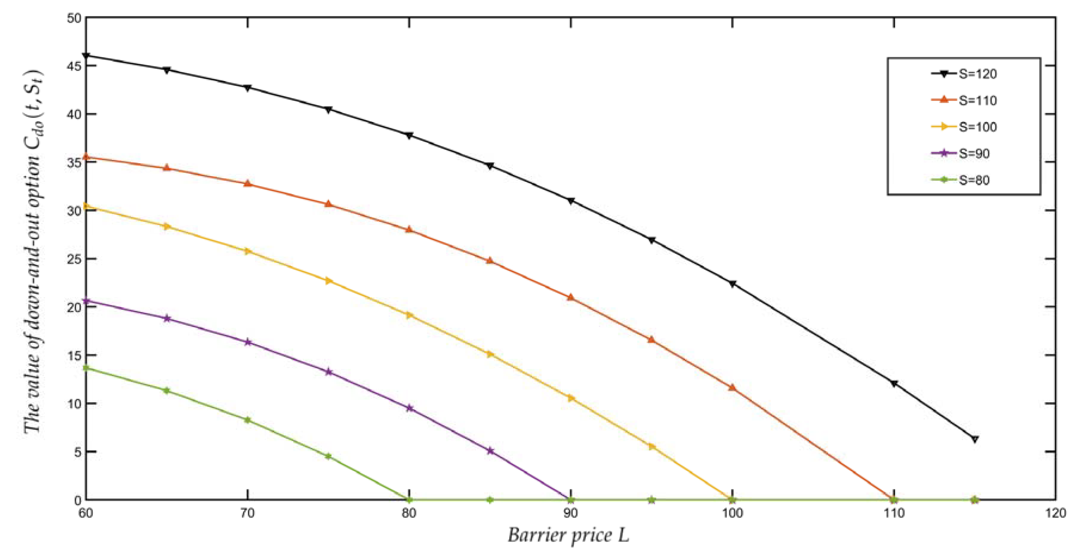
According to Theorem 4, the value of down-and-out call option $C_{do}(t,S_t)$ under different barrier prices and stock prices can be obtained, which are given in

Table 1. The value of down-and-out options for different barrier prices and stock prices.

L	${\mathit{S}}_0=120$	${\mathit{S}}_0=110$	${\mathit{S}}_0=100$	${\mathit{S}}_0=90$	${\mathit{S}}_0=80$
115	6.350	–	–	–	–
110	12.112	0.000	–	–	–
100	22.445	11.591	0.000	–	–
95	26.969	16.541	5.534	–	–
90	31.042	20.926	10.551	0.000	–
85	34.654	24.731	15.095	5.086	–
80	37.803	27.956	19.149	9.510	0.000
75	40.495	30.613	22.702	13.264	4.507
70	42.748	32.730	25.757	16.351	8.275
65	44.587	34.352	28.324	18.798	11.321
60	46.049	35.533	30.430	20.653	13.680

. At the same time, Figure 1 is drawn to describe the trend of option value affected by barrier price under different stock prices.

Observing Table 1 and Figure 1, it can be seen that when the stock price is fixed, the value of down-and-out call option decreases with the growth of barrier price. When other conditions remain unchanged, with the rising barrier price, the possibility of down-and-out call option termination is increasing, so the option value will continue to decline. In particular, when the barrier price increases to the initial stock price, the option will be knocked out at once, which means it has no value any more.

Then, in order to discuss the impact of the Hurst index H and the jump intensity $\lambda$ on the option price, a new hypothesis is proposed as follows:

$$t=0,T=0.5,K=100,L=70,\alpha =\beta =\gamma =0.4.$$

Take the different H, $\lambda$, and other assumptions remain unchanged to obtain the option value under various conditions, as shown in

Table 2. The value of down-and-out option for different Hurst index and jump intensity.

${\mathit{S}}_0$	$\mathit{H}=0.75$			$\mathit{H}=0.85$			$\mathit{H}=0.95$
	$\mathbf{\lambda }=\mathbf{0}$	$\mathbf{\lambda }=\mathbf{2}$	$\mathbf{\lambda }=\mathbf{4}$	$\mathbf{\lambda }=\mathbf{0}$	$\mathbf{\lambda }=\mathbf{2}$	$\mathbf{\lambda }=\mathbf{4}$	$\mathbf{\lambda }=\mathbf{0}$	$\mathbf{\lambda }=\mathbf{2}$	$\mathbf{\lambda }=\mathbf{4}$
120	31.119	36.621	40.017	29.761	35.812	39.501	28.472	35.045	39.018
115	27.257	32.652	35.839	25.860	31.879	35.360	24.500	31.141	34.910
110	23.554	28.760	31.708	22.144	28.033	31.270	20.737	27.334	30.857
105	20.024	24.949	27.626	18.632	24.278	27.232	17.212	23.628	26.859
100	16.679	21.217	23.590	15.344	20.613	23.244	13.953	20.025	22.916
95	13.524	17.563	19.600	12.291	17.038	19.305	10.982	16.522	19.026
90	10.559	13.982	15.650	9.479	13.545	15.411	8.311	13.115	15.183
85	7.770	10.462	11.734	6.895	10.125	11.553	5.935	9.791	11.380
80	5.129	6.988	7.842	4.510	6.759	7.722	3.821	6.531	7.606
75	2.582	3.534	3.959	2.259	3.418	3.900	1.896	3.302	3.843

.

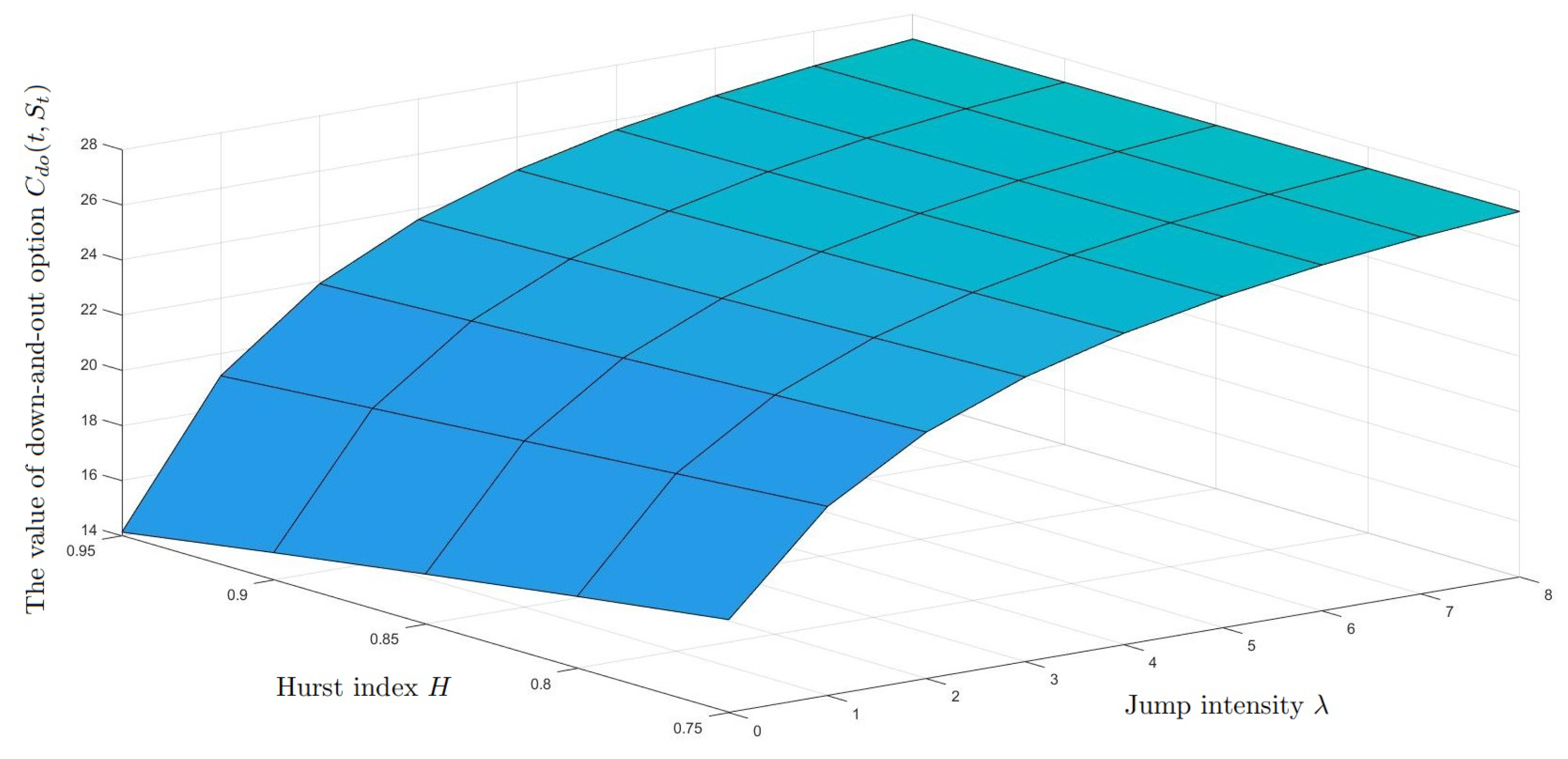
Figure 2 is the variation diagram of the value of down-and-out call option with the different Hurst index and jump intensity, when $S_0$ is fixed at 100. The relationships between the value of down-and-out option and the Hurst index is positive. The larger the Hurst index is, the more stable the underlying asset price is. This means the price fluctuation will be smaller, which denotes the corresponding option value will be smaller.

At the same time, the value of down-and-out option and the jump intensity change in the same direction. The jump intensity represents the unsystematic risk. When it increases, the underlying asset will has more intense fluctuations, which means higher upper limit and invariant lower bound. Therefore, the option value will rise.

Finally, for rigorousness, we verify the positive correlation between the volatility and the value of down-and-out call option, where $\alpha ,\beta ,and\gamma$ are different. Assume that the parameter selection is as follows:

$$t=0,T=0.5,K=100,L=70,H=0.75,\lambda =1.$$

Let $\widehat{\sigma }=(\alpha ,\beta ,\gamma )$, and make

$${\widehat{\sigma }}_1=(0.1,0.15,0.2);{\widehat{\sigma }}_2=(0.2,0.25,0.3);{\widehat{\sigma }}_3=(0.3,0.35,0.4);{\widehat{\sigma }}_4=(0.4,0.45,0.5).$$

According to Theorem 4, the value of down-and-out call option under different volatility can be obtained, which are shown in

Table 3. The value of down-and-out option against the volatility of the underlying asset.

${\mathit{S}}_0$	${\widehat{\mathit{\sigma }}}_1=$ (0.1, 0.15, 0.2)	${\widehat{\mathit{\sigma }}}_2=$ (0.2, 0.25, 0.3)	${\widehat{\mathit{\sigma }}}_3=$ (0.3, 0.35, 0.4)	${\widehat{\mathit{\sigma }}}_4=$ (0.4, 0.45, 0.5)
120	25.323	28.441	32.360	36.149
115	20.918	24.467	28.506	32.202
110	16.770	20.702	24.790	28.338
105	12.963	17.176	21.222	24.559
100	9.581	13.917	17.807	20.867
95	6.704	10.948	14.549	17.259
90	4.385	8.281	11.443	13.729
85	2.637	5.910	8.477	10.267
80	1.416	3.803	5.623	6.856
75	0.608	1.886	2.838	3.467

. The value of down-and-out call option increases with the rise of the volatility, which is consistent with the fact.

6. Conclusions

This paper investigated the barrier option pricing model in the environment of the sub-mixed fractional Brownian motion with jump intensity. Through the self-financing strategy, we derive the B-S type PDE of the derivatives. Then, the value of the down-and-out option is obtained by applying transformation techniques. Meanwhile, the parity formula between barrier call option and barrier put option can be given by a similar method. Next, using the linear relationship between the knock-out option and the knock-in option, the value of the knock-in option can be deduced. In Section 5, the numerical experiment is carried out where we take the down-and-out call option as an example. According to the results shown in Figure 1, Figure 2, and Table 3, the following relationships can be found: The barrier price and Hurst index are inversely related to the value of the down-and-out call option, while the jump intensity and volatility are positively correlated with it. In the above numerical experiment, the parameter values are averages. It may affect the application of the model according to reference [32], and we will try our best to overcome this limitation in future research. Meanwhile, the Asian barrier options can also be considered to extend the model used in this paper.

References

- Dassios, A.; Lim, J.W. Recursive formula for the double-barrier Parisian stopping time. J. Appl. Probab. 2018, 55, 282–301. [Google Scholar] [CrossRef]
- Funahashi, H.; Higuchi, T. An analytical approximation for single barrier options under stochastic volatility models. Ann. Oper. Res. 2018, 266, 129–157. [Google Scholar] [CrossRef]
- Guillaume, T. Closed form valuation of barrier options with stochastic barriers. Ann. Oper. Res. 2021, 1–30. [Google Scholar] [CrossRef]
- Gao, Y.; Jia, L. Pricing formulas of barrier-lookback option in uncertain financial markets. Chaos Solitons Fractals 2021, 147, 110986. [Google Scholar] [CrossRef]
- Shreve, S.E. Stochastic Calculus for Finance II: Continuous-Time Models; Springer: New York, NY, USA, 2004. [Google Scholar]
- Merton, R.C. Theory of rational option pricing. Bell Econ. Manag. Sci. 1973, 4, 141–183. [Google Scholar] [CrossRef] [Green Version]
- Rubinstein, M. Breaking down the barriers. Risk 1991, 4, 28–35. [Google Scholar]
- Black, F.; Scholes, M. The Pricing of Options and Corporate Liabilities. J. Political Econ. 1973, 81, 637–654. [Google Scholar] [CrossRef] [Green Version]
- Ding, Z.; Granger, C.W.; Engle, R.F. A long memory property of stock market returns and a new model. J. Empir. Financ. 1993, 1, 83–106. [Google Scholar] [CrossRef]
- Shiryaev, A.N. Essentials of Stochastic Finance: Facts, Models, Theory; World Scientific: Singapore, 1999. [Google Scholar]
- Necula, C. Option pricing in a fractional Brownian motion environment. Adv. Econ. Financ. Res.-Dofin Work. Pap. Ser. 2008, 2, 259–273. [Google Scholar] [CrossRef]
- Kolmogorov, A.N. Wienersche spiralen und einige andere interessante kurven in hilbertscen raum, cr (doklady). Acad. Sci. URSS (NS) 1940, 26, 115–118. [Google Scholar]
- Chen, Q.; Zhang, Q.; Liu, C. The pricing and numerical analysis of lookback options for mixed fractional Brownian motion. Chaos Solitons Fractals 2019, 128, 123–128. [Google Scholar] [CrossRef]
- Bian, L.; Li, Z. Fuzzy simulation of European option pricing using sub-fractional Brownian motion. Chaos Solitons Fractals 2021, 153, 111442. [Google Scholar] [CrossRef]
- Wang, J.; Yan, Y.; Chen, W.; Shao, W.; Tang, W. Equity-linked securities option pricing by fractional Brownian motion. Chaos Solitons Fractals 2021, 144, 110716. [Google Scholar] [CrossRef]
- Cheridito, P. Arbitrage in fractional Brownian motion models. Financ. Stochastics 2003, 7, 533–553. [Google Scholar] [CrossRef]
- Bender, C.; Elliott, R.J. Arbitrage in a discrete version of the Wick-fractional Black-Scholes market. Math. Oper. Res. 2004, 29, 935–945. [Google Scholar] [CrossRef]
- Björk, T.; Hult, H. A note on Wick products and the fractional Black-Scholes model. Financ. Stochastics 2005, 9, 197–209. [Google Scholar] [CrossRef]
- Bojdecki, T.; Gorostiza, L.G.; Talarczyk, A. Sub-fractional Brownian motion and its relation to occupation times. Stat. Probab. Lett. 2004, 69, 405–419. [Google Scholar] [CrossRef]
- Charles, E.N.; Mounir, Z. On the sub-mixed fractional Brownian motion. Appl.-Math.-J. Chin. Univ. 2015, 30, 27–43. [Google Scholar] [CrossRef] [Green Version]
- Tudor, C. Some properties of the sub-fractional Brownian motion. Stochastics Int. J. Probab. Stoch. Process. 2007, 79, 431–448. [Google Scholar] [CrossRef]
- Xu, F.; Zhou, S. Pricing of perpetual American put option with sub-mixed fractional Brownian motion. Fract. Calc. Appl. Anal. 2019, 22, 1145–1154. [Google Scholar] [CrossRef]
- Merton, R.C. Option pricing when underlying stock returns are discontinuous. J. Financ. Econ. 1976, 3, 125–144. [Google Scholar] [CrossRef] [Green Version]
- Zhou, Q.; Yang, J.J.; Wu, W.X. Pricing vulnerable options with correlated credit risk under jump-diffusion processes when corporate liabilities are random. Acta Math. Appl. Sin. Engl. Ser. 2019, 35, 305–318. [Google Scholar] [CrossRef]
- Sun, W.; Zhao, Y.; MacLean, L. Real Options in a Duopoly with Jump Diffusion Prices. Asia-Pac. J. Oper. Res. 2021, 38, 2150009. [Google Scholar] [CrossRef]
- Zhang, W.G.; Li, Z.; Liu, Y.J.; Zhang, Y. Pricing European option under fuzzy mixed fractional Brownian motion model with jumps. Comput. Econ. 2021, 58, 483–515. [Google Scholar] [CrossRef]
- Liu, M. Two possible types of superfluidity in crystals. Phys. Rev. B 1978, 18, 1165. [Google Scholar] [CrossRef]
- Callen, H.B. Thermodynamics and an Introduction to Thermostatistics; John Wiley & Sons: New York, NY, USA, 1985. [Google Scholar]
- Appel, D.; Grabinski, M. The origin of financial crisis: A wrong definition of value. Port. J. Quant. Methods 2011, 2, 33. [Google Scholar]
- Klinkova, G.; Grabinski, M. Conservation laws derived from systemic approach and symmetry. Int. J. Latest Trends Fin. Ecol. Sci. Vol. 2017, 7, 1307. [Google Scholar]
- Tankov, P. Financial Modelling with Jump Processes; Chapman and Hall/CRC: London, UK, 2003. [Google Scholar]
- Grabinski, M.; Klinkova, G. Wrong use of averages implies wrong results from many heuristic models. Appl. Math. 2019, 10, 605. [Google Scholar] [CrossRef] [Green Version]
Publisher’s Note: MDPI stays neutral with regard to jurisdictional claims in published maps and institutional affiliations. |
© 2022 by the authors. Licensee MDPI, Basel, Switzerland. This article is an open access article distributed under the terms and conditions of the Creative Commons Attribution (CC BY) license (https://creativecommons.org/licenses/by/4.0/).