Design and High-Order Precision Numerical Implementation of Fractional-Order PI Controller for PMSM Speed System Based on FPGA

Abstract

In this paper, the design of a fractional-order proportional integral (FOPI) controller and integer-order (IOPI) controller are compared for the permanent magnet synchronous motor (PMSM) speed regulation system. A high-precision implementation method of a fractional-order proportional integral (FOPI) controller is proposed in this work. Three commonly used numerical implementation methods of fractional operators are investigated and compared for comprehensively evaluating the numerical implementation performance in this work. Furthermore, for the impulse response invariant implementation method, the effects of different discretization orders on the control performance of the system are compared. The high-order fractional-order controller can be implemented accurately in a control system with the field-programmable gate array (FPGA) with the capability of parallel calculation. The simulation and experimental results show that the high-precision numerical implementation method of the designed high-order FOPI controller has better performance than the ordinary precision fractional operation implementation method and traditional order integer order PI controller.

1. Introduction

As a generalization of integer calculus, fractional calculus can describe the actual physical objects more accurately. Fractional calculus has attracted more and more attention in engineering and physics, such as physical modeling, controller design [1,2,3], chaotic systems [4,5], and so on [6]. In the field with specific characteristics such as viscoelasticity and friction, fractional calculus can be used to describe some important applications [7]. Moreover, the fractional-order controller has more parameters and can improve the overall performance of the control systems, such as robustness and disturbance rejection [3,8]. Field-Programmable Gate Array (FPGA) has been widely used for digital system implementation due to its concurrency, programmability, and short development cycle [9,10,11,12,13]. Regardless of the complexity of the control algorithm, the computation cycle of controller based on FPGA can be relatively short compared to a pipelined digital signal processor (DSP) and personal computer (PC) because of its parallel architecture [14]. The implementation of the servo system based on FPGA can achieve high performance such as high bandwidth and good dynamic response performance [15,16]. A high-precision digital proportional integral derivative (PID) controller based on FPGA is implemented in [17].

A permanent magnet synchronous motor (PMSM) has advantages of high power, low loss, and high efficiency, providing the desired control performance and flexibility [18]. The field-oriented control (FOC) algorithm is generally regarded as a good method to control the PMSM. It has been applied in many fields, such as industrial robots, precision machining platforms, and so on. In view of the coupling, time-varying, and other nonlinear characteristics of PMSM, fractional-order controllers can achieve better control performance over traditional controllers [19,20,21].

The discretization of the fractional order operator is essential for fractional-order numerical implementation. The mathematical problems are more complex for a fractional-order integrator/differentiator than an integer-order integrator/differentiator. Ideally, an integer-order transfer function containing infinite poles and zeros is required to implement a fractional-order transfer function, which is impossible in practical systems. However, the proper approximation can be obtained with finite zeros and poles. Due to resource and computing time constraints, fractional-order discretization order is usually less than 7th in the microprocessor system. In [22], a fractional-order active disturbance rejection controller (FOADRC) is proposed for the speed servo system of PMSM, which has good tracking and anti-load disturbance performance. Experimental verification is carried out based on the DSP platform with the 5th fractional discretization order. In [23], a fractional-order proportional integral derivative (FOPID) controller is used to control the position of suspended objects in a magnetic levitation system (MLS), which has a better position accuracy with fewer efforts than conventional methods. In addition, the fractional-order operator is implemented with the 7th-order discretization with Visual C. Therefore, the traditional microprocessors are limited by resources and algorithm running time, and it is challenging to realize high-order discretization fractional operators. Many researchers study the numerical discretization of fractional-order operators based on FPGA implementation. In [24,25], a fractional-order discretization method is proposed based on the Grunwald Letnikov (GL) definition, which is numerically discretized based on FPGA implementation and applied to practical fractional-order systems. This method effectively reduces the memory dependence of fractional order operators, but it can only have a good fitting effect of a fractional-order operator in a small frequency range. In [26], a fractional-order operators discretization method is proposed based on the GL definition using the piecewise linear approximation algorithm. The implementation is based on FPGA with better fitting accuracy and high FPGA resource utilization. However, the effective fitting frequency range of the fractional operator is still tiny. A few people have studied and compared the FPGA implementation performance of fractional operators with other commonly used methods.

In this paper, the high-precision numerical implementation of FOPI is carried out based on FPGA. Based on the PMSM model, an FOPI controller is designed with the given frequency domain index for the speed control of PMSM. The influential factors of discretization accuracy are investigated, including different discretization methods and discretization orders. The field-oriented control method is realized based on FPGA. Experimental results show that the high-precision numerical implementation method has better dynamic response characteristics and robustness.

The main contributions of this paper are as follows: (1) Three commonly used fractional-order operator discretization methods are compared in the frequency-domain, including the impulse response invariant method, Oustaloup method, and GL method. Furthermore, the fitting effects are investigated with different discretization orders of three methods. (2) The numerical implementation method of the field-oriented control and the high-precision FOPI controller is proposed based on FPGA, which can achieve higher precision with less time delay. (3) PMSM speed servo simulation and experimental results are presented to show the control performance advantages of the designed high-order FOPI controller based on FPGA.

The research process of this paper is shown in Figure 1. We introduce the design of the FOPI controller in Section 2. Section 3 presents the comparison of numerical implementation methods of fractional order operators. Section 4 demonstrates the simulation analysis of PMSM speed control performance of different controllers. Section 5 introduces the FPGA structure design and the experimental research. Finally, we give the conclusion in Section 6.

2. The Plant Model and Controller Design

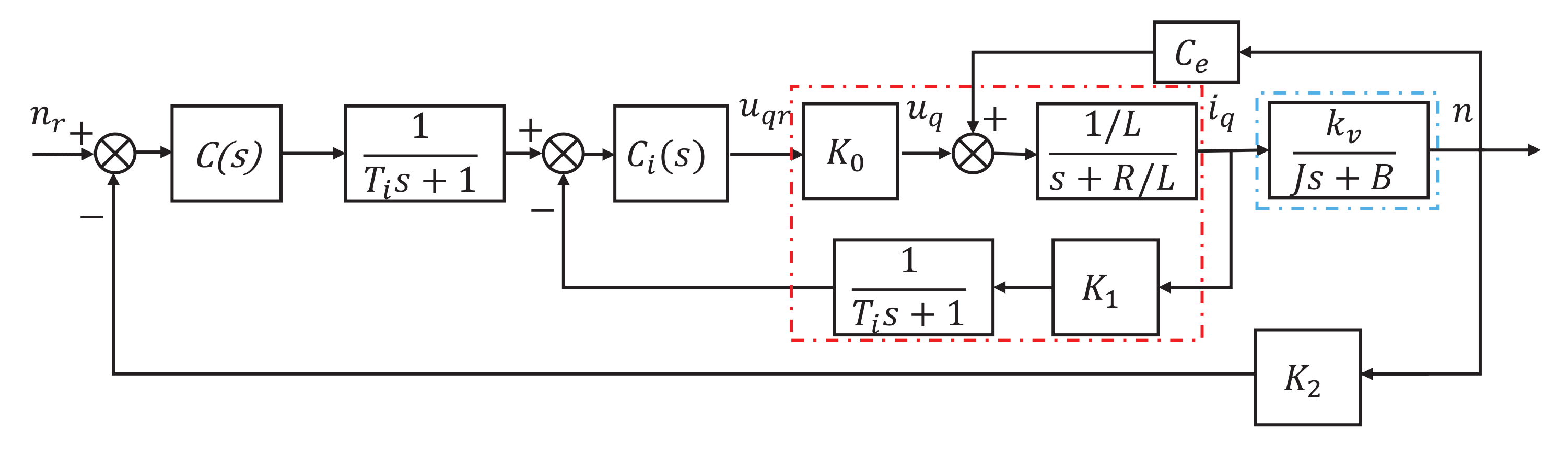
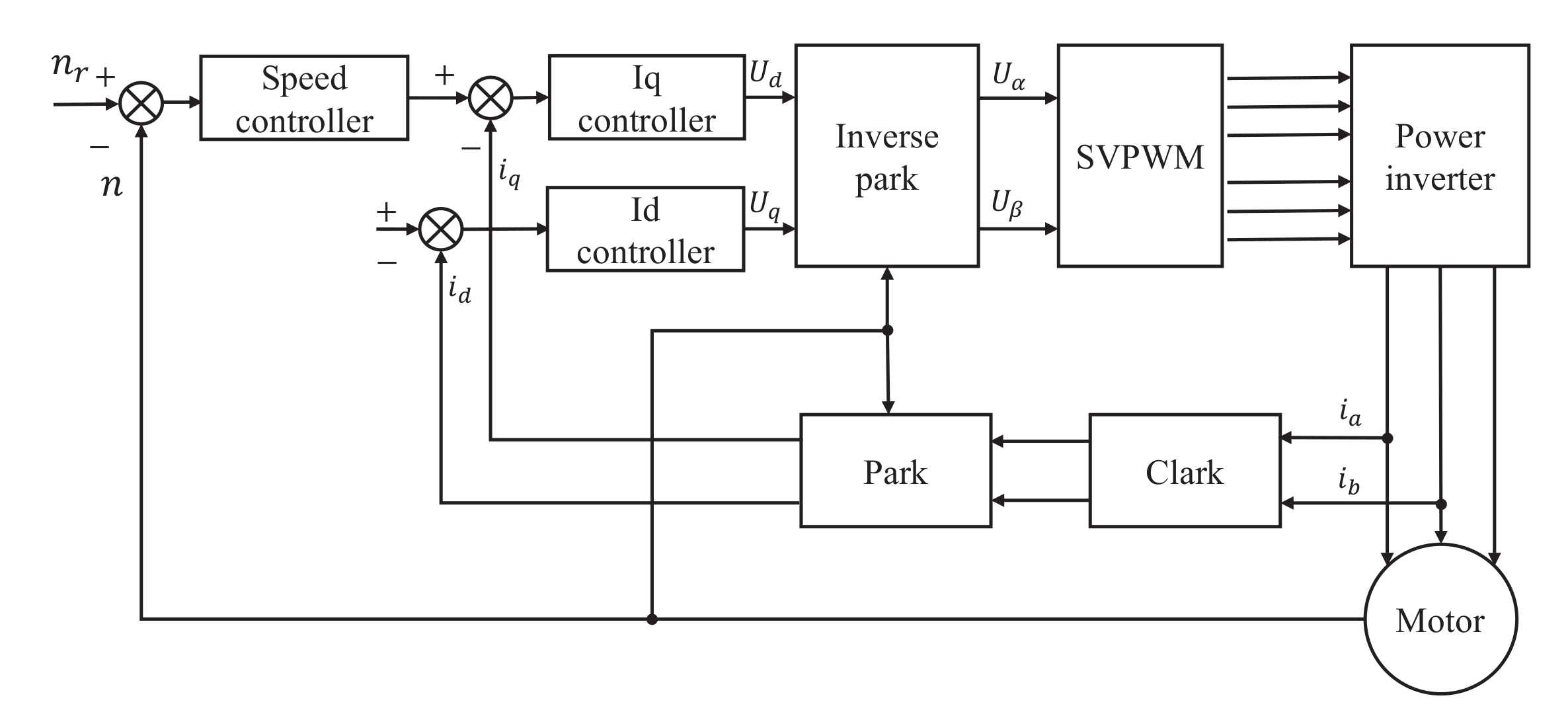
2.1. The Plant Model of PMSM Servo System

In this paper, the speed loop of PMSM is taken as the controlled object. Figure 2 is the PMSM speed servo system, where $C\left(s\right)$ and $C_i\left(s\right)$ are the speed controller and the current controller. $K_0$, $K_1$, and $K_2$ are the voltage, current, and speed conversion factors, respectively. $T_i$ is the current filter coefficient. The red dotted block and blue dotted block are electromagnetic components and mechanical components. The electromagnetic part can be described by

$$u_q-E=u_q-C_{e}n=R{i}_q+L\frac{d{i}_q}{dt},$$

(1)

where $u_q$ is the q axis voltage, E is the electromotive force, $C_e$ is the electromotive force coefficient, n is the speed, $i_q$ is the q axis current, and R and L are the stator equivalent resistance and inductance, respectively. The mechanical part can be described by,

$$T_e-T_L=C_m(i_q-i_L)=\frac{J}{k_m}\frac{dn}{dt}+\frac{B}{k_m}n,$$

(2)

where $T_e$ and $T_L$ are the electromagnetic torque and equivalent torque of the load, $k_m$ = 30/$\pi$, $C_m$ is the torque coefficient, $i_L$ is the equivalent load current, J is the flywheel inertia, and B is the viscosity coefficient.

The transfer functions of the electromagnetic and mechanical parts can be calculated by,

$$G_1\left(s\right)=\frac{I_q}{U_q-E}=\frac{1}{Ls+R},$$

(3)

$$G_2\left(s\right)=\frac{N}{I_q-I_L}=\frac{k_v}{Js+B},$$

(4)

where $k_v$ = $k_m{C}_m$.

A nonlinear identification approach based on output error is adopted to get the model parameters [27]. Based on this method, the electromagnetic part model and mechanical part model can be identified as,

$$G_1\left(s\right)=\frac{415.60}{s+190.4715},$$

(5)

$$G_2\left(s\right)=\frac{2213.5}{s+1.3771}.$$

(6)

In order to reduce the influence of current disturbance, we introduce a first-order digital low-pass filter as follows:

$$G_f\left(s\right)=\frac{1}{T_{i}s+1},$$

(7)

where $T_i$ is the filter coefficient.

The current loop controller model is

$$C_i\left(s\right)=K_{pc}+\frac{K_{ic}}{s}.$$

(8)

where $K_{pc}$ and $K_{ic}$ are proportional and integral coefficients. The open-loop transfer function of the current loop can be seen in Figure 2, and its definition is as follows:

$$P_o\left(s\right)=K_0{K}_1{C}_i\left(s\right)G_1\left(s\right)G_f\left(s\right)=K_0{K}_1\frac{b}{s+a}\left(\frac{K_{pc}s+K_{ic}}{s}\right)\frac{1}{T_{i}s+1}.$$

(9)

In this paper, $K_0$ = 213.667, $K_1$ = 19.2, $K_2$ = 0.0005, and $T_i$ = 0.000318. The current controller is designed by the cancellation method with relationship $K_{pc}/K_{ic}=1/a$. The gain crossover frequency is set as $w_c$ = 3000 rad/s,

$$\left|P_o\left(j{\omega }_c\right)\right|=1.$$

(10)

The current loop controller model can be obtained as follows:

$$C_i\left(s\right)=0.8971+\frac{170.8720}{s}.$$

(11)

Based on the principle of FOC, the parameters of the $Iq$ controller and $Id$ controller are the same. So, the plant model of the PMSM speed control system is as follows,

$$P\left(s\right)=\frac{2.76847\times {10}^8}{s^3+3141.38s^2+1.30327\times {10}^{7}s+1.79413\times {10}^7}.$$

(12)

2.2. The Controller Design

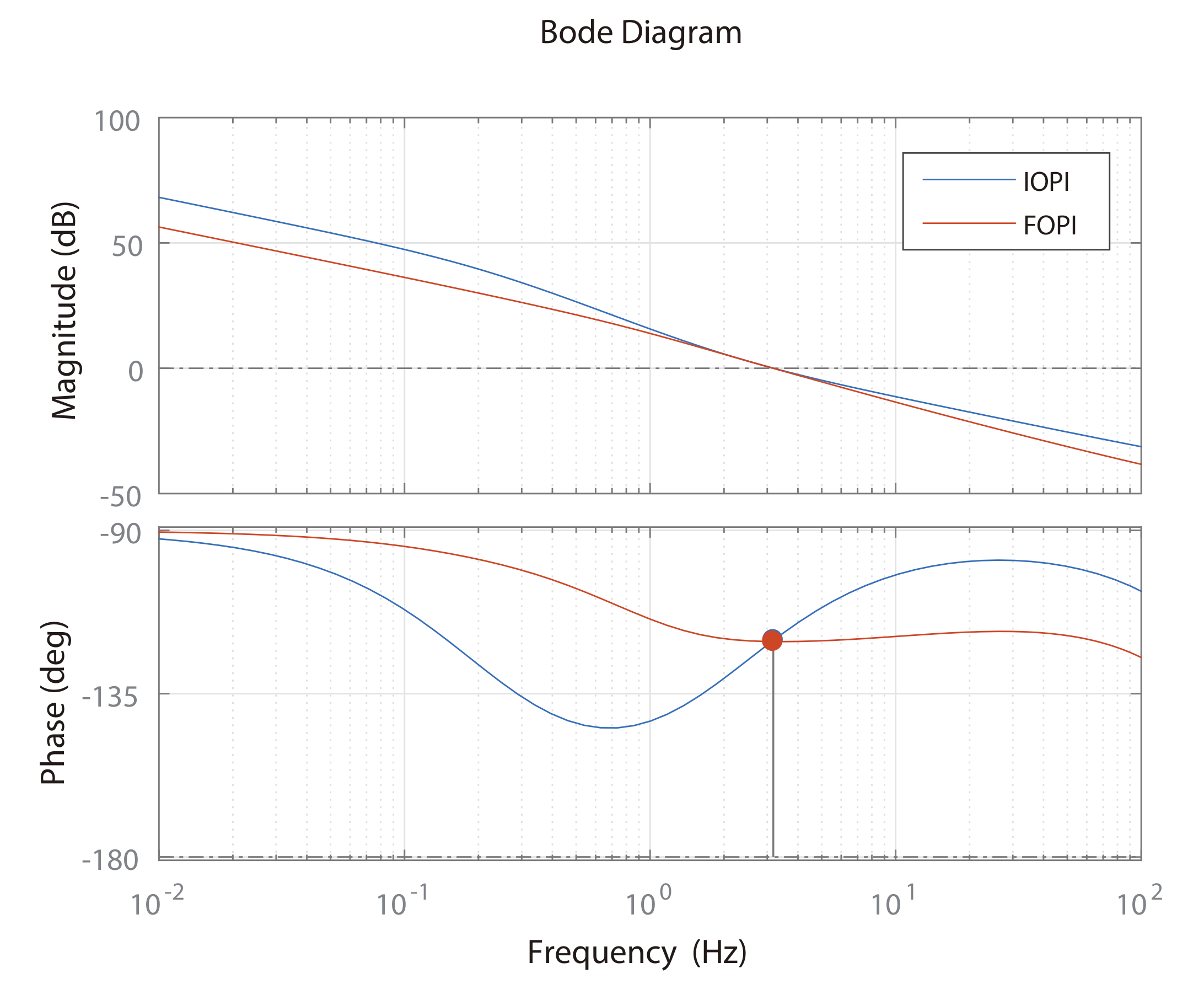
2.2.1. Fractional Order PI Controller Design

Compared with the traditional linear PI controller, FOPI has more flexibility in parameters adjustment, including the fractional order. In order to make the speed control of PMSM robust to loop gain variation, an FOPI controller is considered with the structure as,

$$C\left(s\right)=K_P\left(1+\frac{K_i}{s^{\alpha }}\right),$$

(13)

where $K_P$ is the proportional gain, $K_i$ is the integral gain, and $\alpha$ is the order of the integration. The open-loop transfer function $G_s\left(s\right)$ can be written as,

$$G_s\left(s\right)=C\left(s\right)P\left(s\right).$$

(14)

The controller $C\left(s\right)$ contains three unknown parameters. The gain crossover frequency is given as ${\omega }_c$, and the phase margin is given as ${\varphi }_m$. Three specifications are imposed as follows,

(1) Phase margin specification,

$$Arg\left[G\left(j{\omega }_c\right)\right]=Arg\left[C\left(j{\omega }_c\right)P\left(j{\omega }_c\right)\right]=-\pi +{\varphi }_m.$$

(15)

(2) Gain crossover frequency specification,

$$\left|G\left(j{\omega }_c\right)\right|=\left|C\left(j{\omega }_c\right)P\left(j{\omega }_c\right)\right|=1.$$

(16)

(3) Flat phase specification,

$${\left|\frac{\mathrm{d}\left(Arg\right(G\left(j\omega \right)\left)\right)}{\mathrm{d}\omega }\right|}_{\omega =\omega c}=0.$$

(17)

The flat phase specification demands the phase is flat around the gain crossover frequency ${\omega }_c$. It means that the system is robust to loop gain variation and maintains a constant overshoot as the gain changes.

The control design specifications are set as ${\varphi }_m$ = ${60}^{\circ }$ and ${\omega }_c$ = 20 rad/s. By calculation, the intersection value of $K_i$ and $\alpha$ is obtained as $K_P=0.252623$, $K_i=3.28026$, and $\alpha =0.494177$. The open-loop Bode diagram is obtained, which meets the design index, as shown in Figure 3. The dots with different colors in the figure represent the phase at the gain crossover frequency.

2.2.2. Integer-Order PI Controller Design

In order to compare with the fractional-order controller, we also design an integer-order proportional intregral (IOPI) controller for the PMSM system. The structure of the IOPI controller is,

$$C_2\left(s\right)=K_p+\frac{K_i}{s},$$

(18)

where $K_P$, $K_i$ are the parameters for proportional and integral items. The open-loop transfer function $G_2\left(s\right)$ with plant and IOPI controller can be written as,

$$G_2\left(s\right)=C_2\left(s\right)P\left(s\right).$$

(19)

The phase margin and gain crossover frequency are,

$$\begin{array}{c}\hfill Arg\left[G_2\left(j{\omega }_c\right)\right]=-\pi +{\varphi }_m,\end{array}$$

(20)

$$\left|G_2\left(j{\omega }_c\right)\right|=\left|C_2\left(j{\omega }_c\right)P\left(j{\omega }_c\right)\right|=1.$$

(21)

The controller of IOPI consists of two unknown control parameters. The control design specifications are set as ${\varphi }_m$ = ${60}^{\circ }$ and ${\omega }_c$ = 20 rad/s. According to the constraint conditions, $K_i=10.4586$, $K_P=0.78521$. The open-loop Bode diagram of $G_2\left(s\right)$ is obtained, which meets the design index, as shown in Figure 3.

3. Numerical Implementation of Fractional Order Operators

The order of the fractional-order operator can be any real number or even a complex number. The basic operator of fractional calculus is ${}_a{D}_t^{\alpha }$ [28], where a and t are the upper and lower limits of the fractional-order operator, and $\alpha$ is the order of the operator. The fractional-order differential and integral of function $f\left(t\right)$ are as follows,

$${}_a{D}_t^{\alpha }f\left(t\right)=\left\{\begin{array}{cc}\frac{d^{\alpha }}{d{t}^{\alpha }}f\left(t\right),\hfill & Re\left(\alpha \right)>0\hfill \\ f\left(t\right),\hfill & Re\left(\alpha \right)=0\hfill \\ {\int }_a^{t}f\left(t\right){\left(d\tau \right)}^{-\alpha },\hfill & Re\left(\alpha \right)<0,\hfill \end{array}\right.$$

(22)

where the operator ${}_a{D}_t^{\alpha }$ represents the $\alpha$ order derivative or integral of the function. It can be seen that a fractional-order operator combines a fractional integral with a fractional differential. Therefore, the integer order is a special case of fractional-order operator. Three of the most commonly used definitions of fractional calculus are Caputo [29], Riemann-Liouville (RL) [30], and Grunwald-Letnikov (GL) [31].

The fractional-order operator $s^{\alpha }$ is an infinite dimensional system and cannot be directly applied to an integer-order system. Therefore, the approximation of fractional-order control systems is very important. The discretization methods of fractional order can be divided into direct discretization and indirect discretization. The idea of a direct discrete method is divided into two parts. The first part is the conversion of a fractional operator from the s-domain to discrete time domain z-domain. The commonly used methods include Euler, Tustin, and Al-Alaoui. The second part is to use a function of finite order in the z-domain to approximate the z-domain model of the operator. The discretization process is realized through a power series expansion (PSE) [32] and continued fraction expansion (CFE) [33]. The indirect discrete method approximates the fractional-order system to a continuous high-order integer-order system, such as the Oustaloup method [34] and Carlson method [35]. In this paper, three commonly used numerical methods are studied: impulse response invariant method, Oustaloup method, and GL discretization method.

3.1. Impulse Response Invariance Method

The impulse response invariance method was proposed for the discretization of fractional order operators [36]. According to the RL definition of fractional order integral, the $\alpha$-order integral of unit impulse function $\delta \left(t\right)$ can be expressed as:

$$g\left(t\right)={}_0{D}_t^{-\alpha }\delta \left(t\right)=\frac{1}{\mathsf{\Gamma }\left(\alpha \right)}{\int }_0^t\frac{\delta \left(\tau \right)}{{(t-\tau )}^{-\alpha +1}}d\tau =\frac{1}{\mathsf{\Gamma }\left(\alpha \right)}{t}^{\alpha -1},$$

(23)

where $g\left(t\right)$ is the impulse response function of fractional-order integral operator $1/s^{\alpha }$. $g\left(t\right)$ is sampled by an ideal pulse sequence with impulse 1, and the sampling signal of the impulse response is obtained as:

$$g^{*}\left(t\right)=g\left(t\right)\sum _{n=-\infty }^{\infty }\delta \left(t-n{T}_s\right)=\sum _{n=-\infty }^{\infty }\frac{1}{\mathsf{\Gamma }\left(\alpha \right)}{\left(n{T}_s\right)}^{\alpha -1},$$

(24)

where $T_s$ is the sampling period. The pulse response sampling signal is modified as,

$$g_m^{*}\left(t\right)=T_s{g}^{*}\left(t\right)=\sum _{n=-\infty }^{\infty }\frac{1}{\mathsf{\Gamma }\left(\alpha \right)}{T}_s^{\alpha }{n}^{\alpha -1}.$$

(25)

The discretization transfer function of the fractional-order integral operator $1/s^{\alpha }$ can be obtained,

$$G\left(z\right)=\frac{{\sum }_{k=0}^{q}b\left[k\right]z^{-k}}{1+{\sum }_{l=1}^{p}a\left[l\right]z^{-l}},$$

(26)

where p and q are the orders of the polynomials.

3.2. Oustaloup Method

The Oustaloup method was developed on the basis of the study of complex calculus operators. In a certain approximation frequency range, the global approximation of the fractional-order operator is realized by assigning the zeros and poles of the integer-order transfer function. Since the frequency characteristic curve of the fractional order operator is a slant line, there is no filter to approach the fractional-order operator on the whole frequency band but only one frequency band. This method has a good fitting effect in the concerned frequency band. However, the disadvantage of this method is that the effect is not ideal in the high-frequency range. Assuming that the band of interest is $\left({\omega }_L,{\omega }_H\right)$ and the number of filters is $2N+1$, the recursive filter can be expressed as:

$$G_f\left(s\right)=K\prod _{k=-N}^N{\frac{s+{\omega }_k}{s+{\omega }_k}}^{\prime }.$$

(27)

The zeros ${\omega }_k^{\prime }$, poles ${\omega }_k$, and gains K of the filter are shown as,

$${\omega }_k^{\prime }={\omega }_L{\left(\frac{{\omega }_H}{{\omega }_L}\right)}^{\frac{k+N+\frac{1}{2}(1-\alpha )}{2N+1}},$$

(28)

$${\omega }_k={\omega }_L{\left(\frac{{\omega }_H}{{\omega }_L}\right)}^{\frac{k+N+\frac{1}{2}(1+\alpha )}{2N+1}},$$

(29)

$$K={\omega }_H^{\alpha }.$$

(30)

3.3. GL Method

The direct discretization of GL with finite memory length is the simplest way to implement fractional operators [33]. The GL fractional order operator is defined as follows:

$${}_a^{GL}{D}_t^{\alpha }f\left(t\right)=\underset{h\to 0}{lim}\frac{1}{h^{\alpha }}\sum _{j=0}^{\lfloor (t-a)/h\rfloor }{W}_j^{\left(\alpha \right)}f(t-jh),$$

(31)

where $W_j^{\left(\alpha \right)}$ is the binomial coefficients and a is the interval superscript.

In order to facilitate the implementation in the control system, the approximated version of the GL definition is given by [24]:

$$\genfrac{}{}{0ex}{}{GL}{t-L}{D}_t^{\alpha }f\left(t\right)=\frac{1}{h^{\alpha }}\sum _{j=0}^L{W}_j^{\left(\alpha \right)}f(t-jh),$$

(32)

where h is the step size, L is the window size (the discretization order), and $W_j^{\left(\alpha \right)}$ is calculated recursively by,

$$W_0^{\left(\alpha \right)}=1,W_j^{\left(\alpha \right)}=\left(1-\frac{\alpha +1}{j}\right)W_{j-1}^{\left(\alpha \right)},j=1,2,3,...$$

(33)

Considering the principle of short memory, the error in calculating the approximated derivative is:

$$\mathsf{\Delta }\left(t\right)=\left|\stackrel{GL}{\mathrm{a}}{D}_t^{\alpha }f\left(t\right)-{}_{\mathrm{t}-\mathrm{L}}^{GL}{D}_t^{\alpha }f\left(t\right)\right|\le \frac{M{L}^{-\alpha }}{\left|\mathsf{\Gamma }\right(1-\alpha \left)\right|},$$

(34)

where $a+L<t<b$ and $\left|f\right(t\left)\right|<M$ when $a<t<b$. It can be seen from the definition that the fitting error will decrease with the increase of window size. From Equation (32), the GL equation can be divided into two steps: first, the binomial coefficients $W_n^{\left(\alpha \right)}$, where all coefficients are multiplied by $\frac{1}{h^{\alpha }}$; second, multiplication is performed between the input and the coefficients.

4. Simulation Analysis

Theoretically, the higher the approximation order is, the higher the approximation accuracy is. However, in the real systems, a high approximation order will significantly affect the operation time and resource occupation in embedded controllers with micro-processors. So, in practical application, the order of approximation is selected based on the trade-off of the control performance requirement and hardware limitation. In this paper, in order to demonstrate the advantages of the high-order implementation of the fractional-order operator on FPGA with parallel calculation, different implementation methods and discretization orders are executed on FPGA for the PMSM control system.

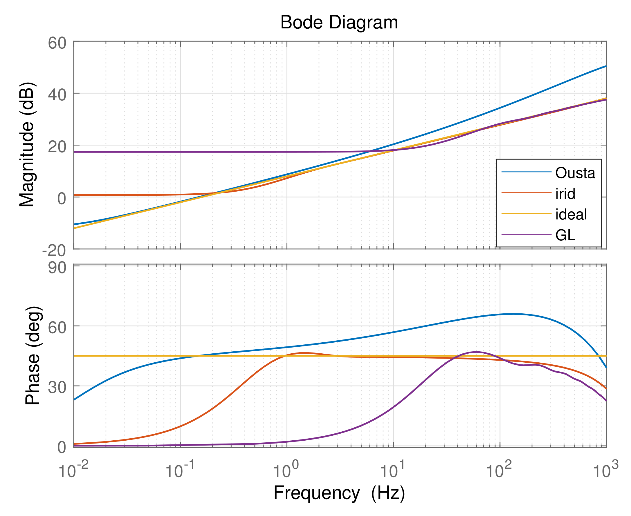
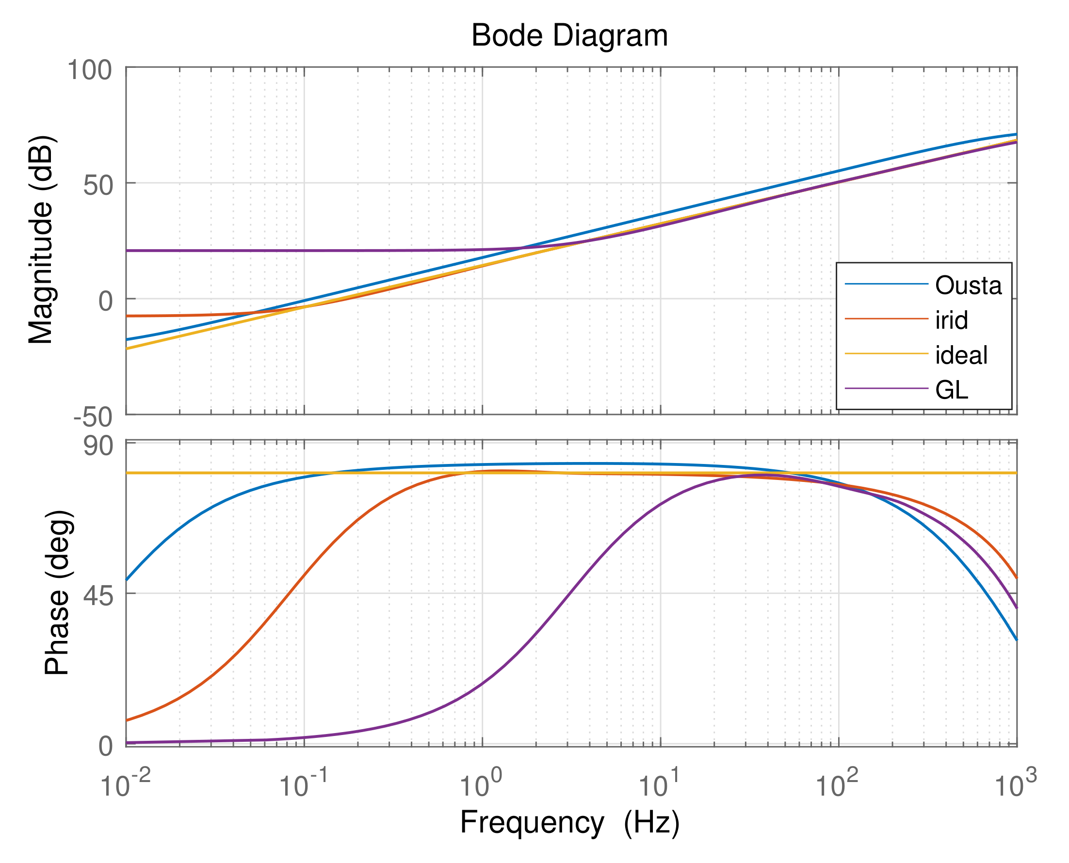
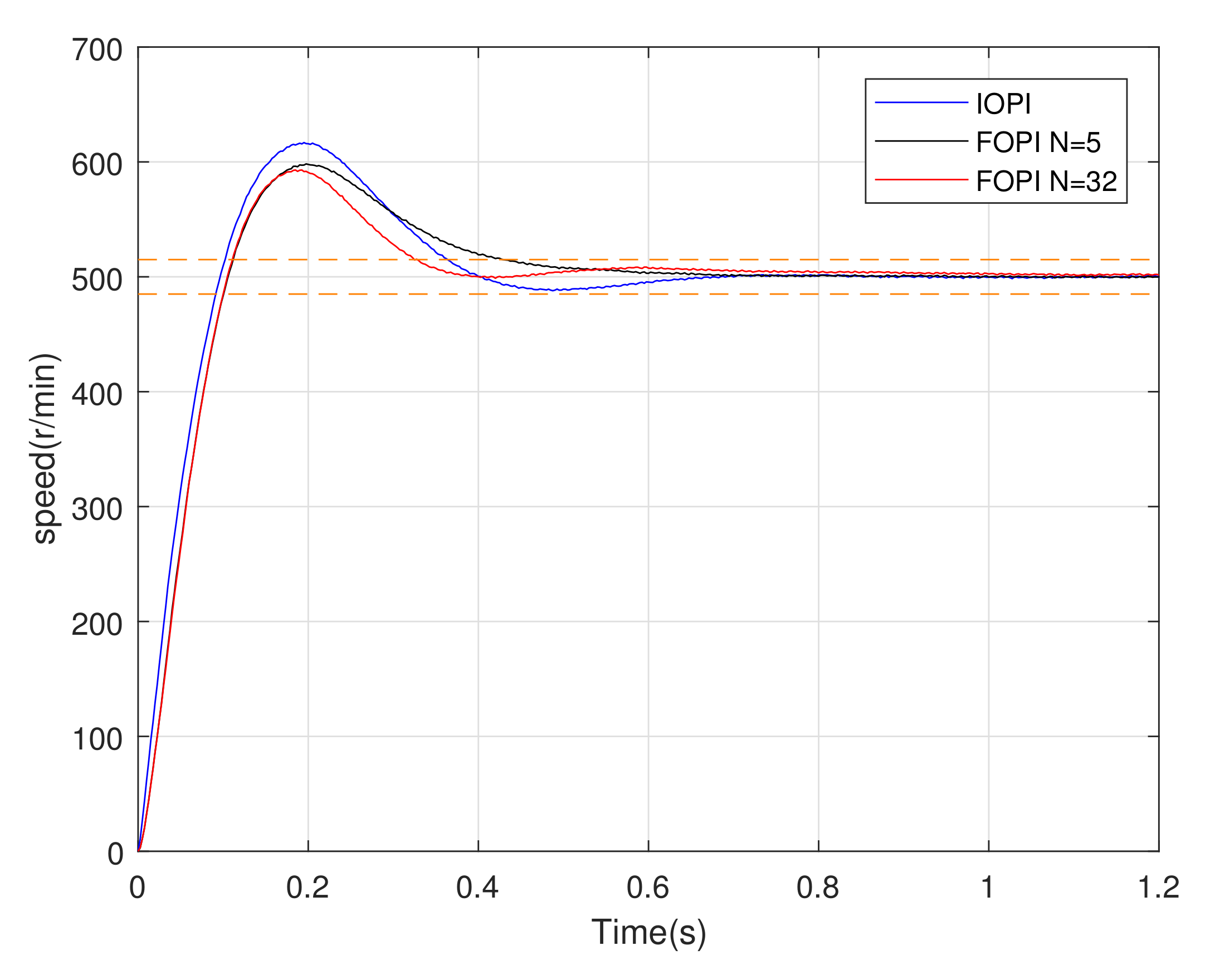
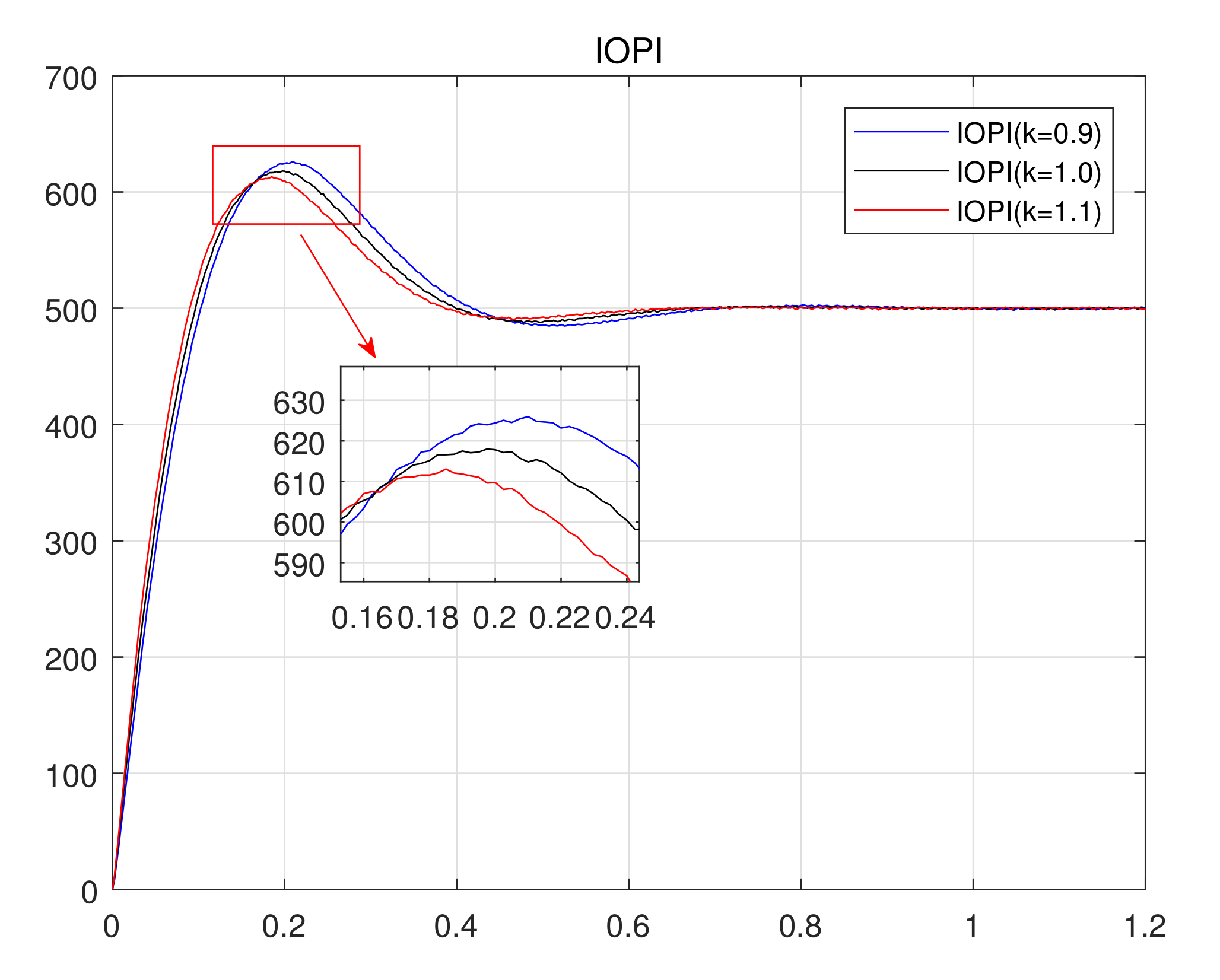
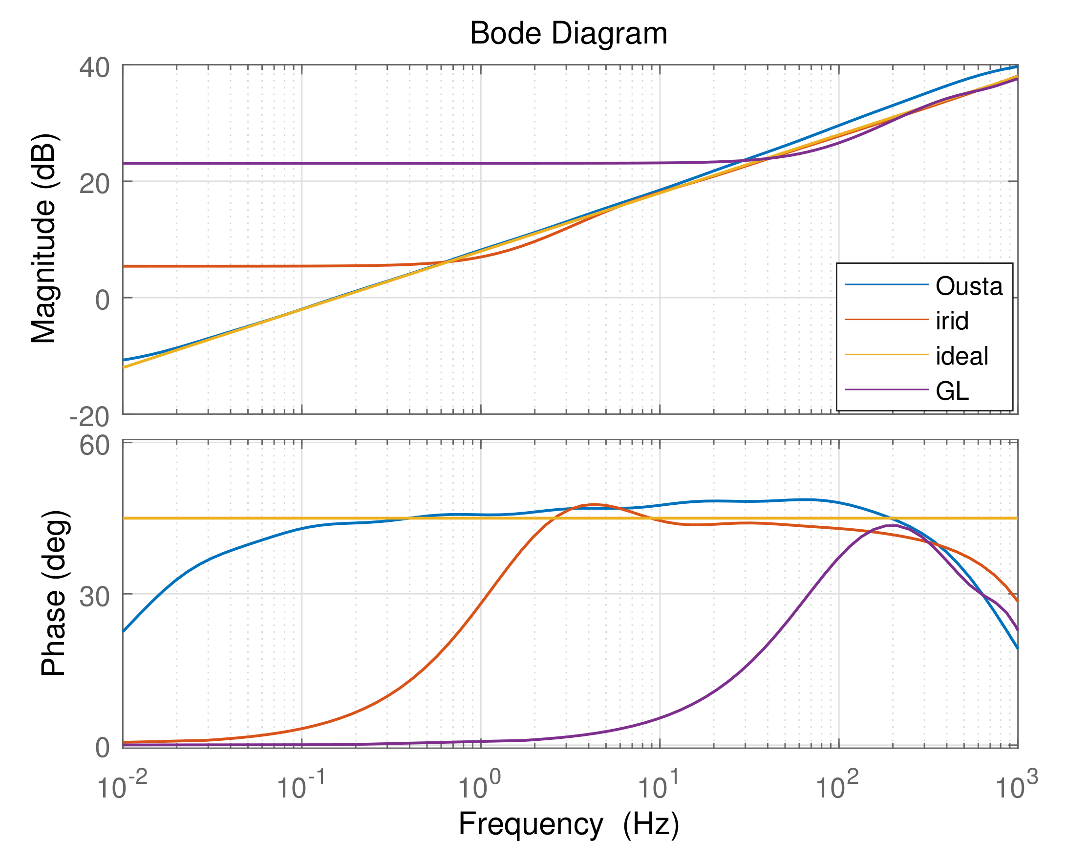
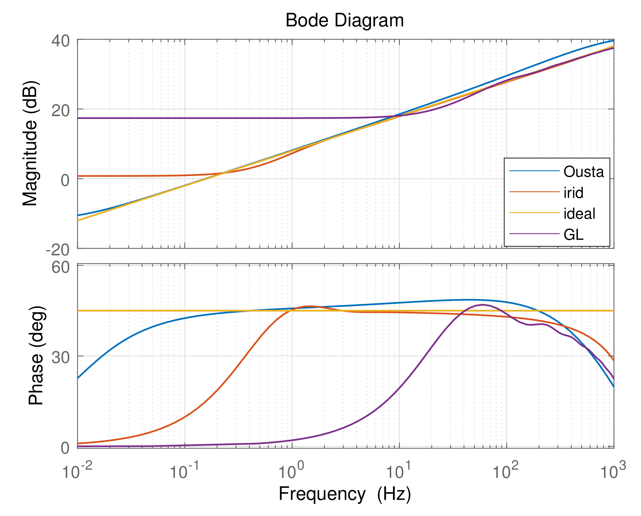
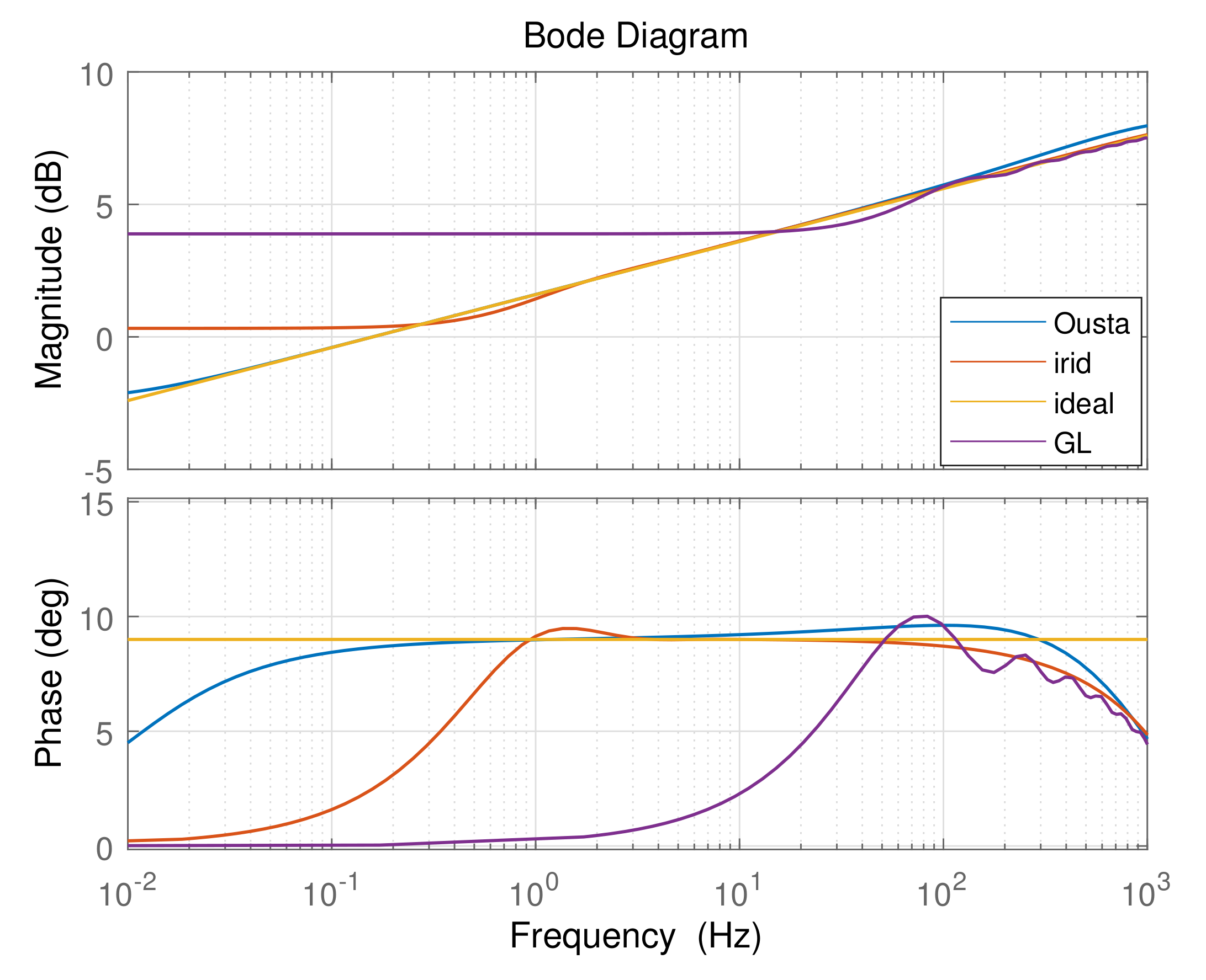
4.1. Comparison of Three Discretization Methods

In order to evaluate the performance of the three numerical methods, given the same discretization order, the results of the three numerical methods are compared. The Bode plots of three fractional operator numerical methods are studied and compared with the ideal value. In order to study the implementation of three fractional-order numerical discretization methods, typical different fractional-order operator orders and frequency bands are given, and the effects of different discretization orders are compared. The designed parameters are shown in

Table 1. Parameters of discretization methods.

	Operator	Considered Frequency	The Discretization
		Band (Hz)	Order N
Case 1	$s^{0.5}$	[0.01,1000]	7
Case 2	$s^{0.5}$	[0.01,1000]	24
Case 3	$s^{0.5}$	[0.01,10,000]	24
Case 4	$s^{0.1}$	[0.01,1000]	24
Case 5	$s^{0.9}$	[0.01,1000]	24

. Considering the actual digital system realization of the PMSM speed loop, the discretization sampling frequency is 4 kHz. The following are the detailed comparisons:

(1) The comparison of case 1 is shown in Figure 4. It can be seen that the fitting performance of the GL definition implementation method is not very close to the ideal value. In this case, the Oustaloup method has a good fitting performance. However, the effect of Oustaloup still has some shortcomings. The fitting error of the phase at high and low frequency is large, and the accuracy of amplitude fitting needs to be improved.

(2) The comparison of case 2 is shown in Figure 5. It can be seen that the fitting effect of the GL definition implementation method is improved. With the increase of discretization order, the fitting effect of the impulse response invariant method is greatly improved. In the amplitude frequency diagram, in the frequency range [3 Hz, 1000 Hz], the impulse response invariant method has higher amplitude frequency fitting accuracy than the Oustaloup method. For the phase, the Oustaloup method has a better fitting performance at low frequency, and the impulse response invariance method has better fitting performance at high frequency.

(3) The comparison of case 3 is shown in Figure 6. Increasing the frequency range of interest [1 Hz, 10,000 Hz], the amplitude and phase fitting accuracy of Oustaloup at high frequency is reduced, while the impulse response invariance method still maintains a good fitting performance.

(4) The comparison of cases 4 and 5 is shown in Figure 7 and Figure 8. The order of the three methods is 24th. The fractional order operators are $s^{0.1}$ and $s^{0.9}$, respectively. It can be seen that with the increase of fractional order at (0,1), the fitting accuracy of the GL method and impulse response invariant method is improved compared with the ideal value. For $s^{0.1}$, the Oustaloup method has a good fitting performance in the case of discretization order 24th. For $s^{0.9}$, in the frequency range [1 Hz, 1000 Hz], the impulse response invariant method has a better amplitude and phase-fitting performance than the Oustaloup method in the case of the 24th discretization order.

For the speed loop control of PMSM, the FOPI controller is implemented by using the impulse response invariance method. The fractional integral operator $1/s^{\alpha }$ can be approximated by an integrator in series with an approximate fractional differential operator. The fractional order integral operator $1/s^{0.494177}$ can be approximated by an integrator in series with an approximate fractional differential operator $s^{0.5058}$. In order to evaluate the influence of the discretization order of the impulse response invariant method on the system performance, different discretization orders (7th and 24th) are given, and their performances are compared. The Bode diagram of fractional order $s^{0.5058}$ is shown in Figure 9. It can be seen that the fitting effect of the 24th is better than that of the 7th, which is closer to the design value at the frequency of 20 rad/s, and the phase is smoother. In Figure 10, the dots with different colors represent the phase at the gain crossover frequency. The gain crossover frequency of the open-loop Bode diagram of the 24th is larger than that of the 7th, which is closer to the design value. The phase of the open-loop Bode diagram corresponding to IOPI at 20 rad/s is not as flat as that for the FOPI controller, so the robustness to loop gain variation for IOPI should not be as good as that for FOPI.

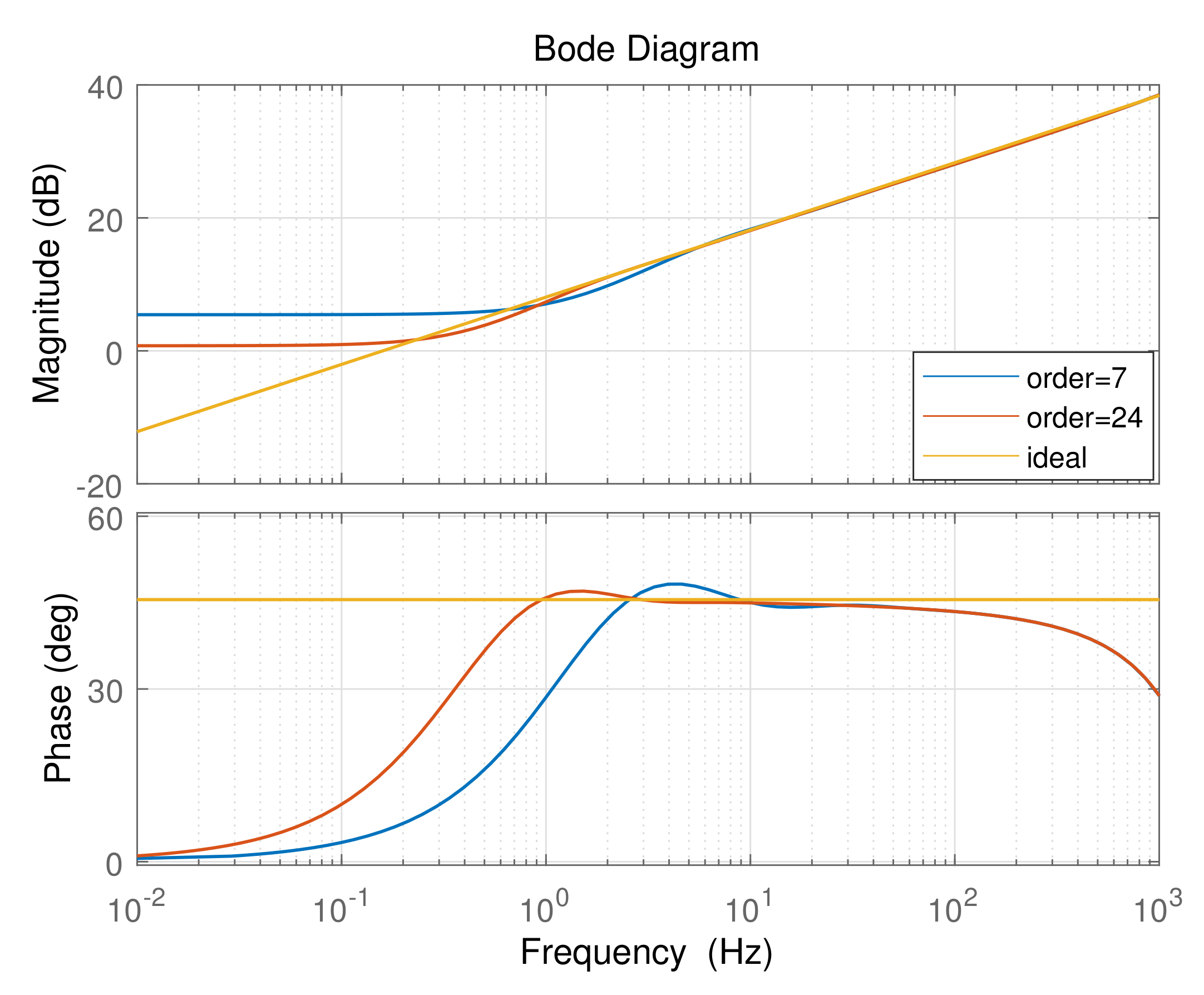
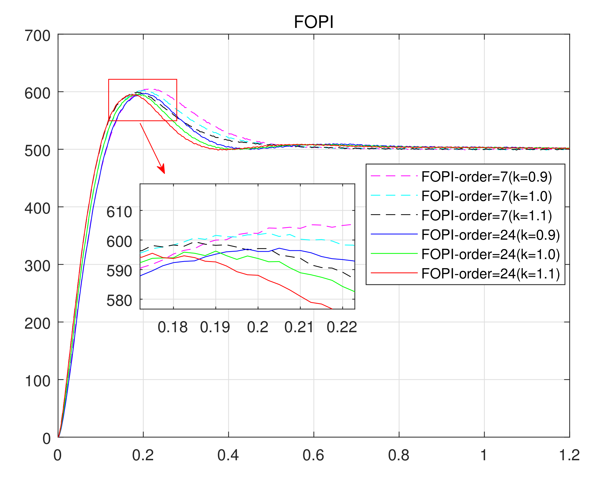
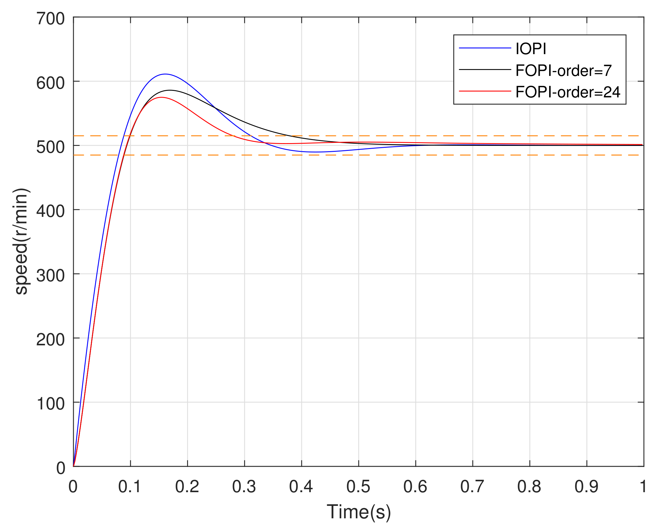
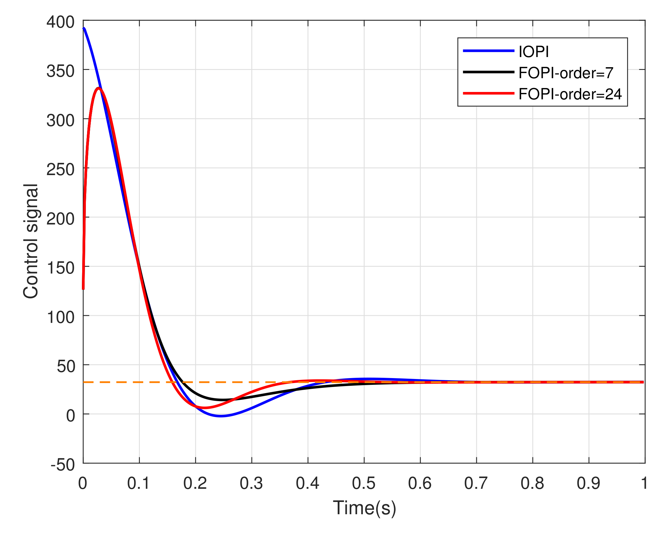
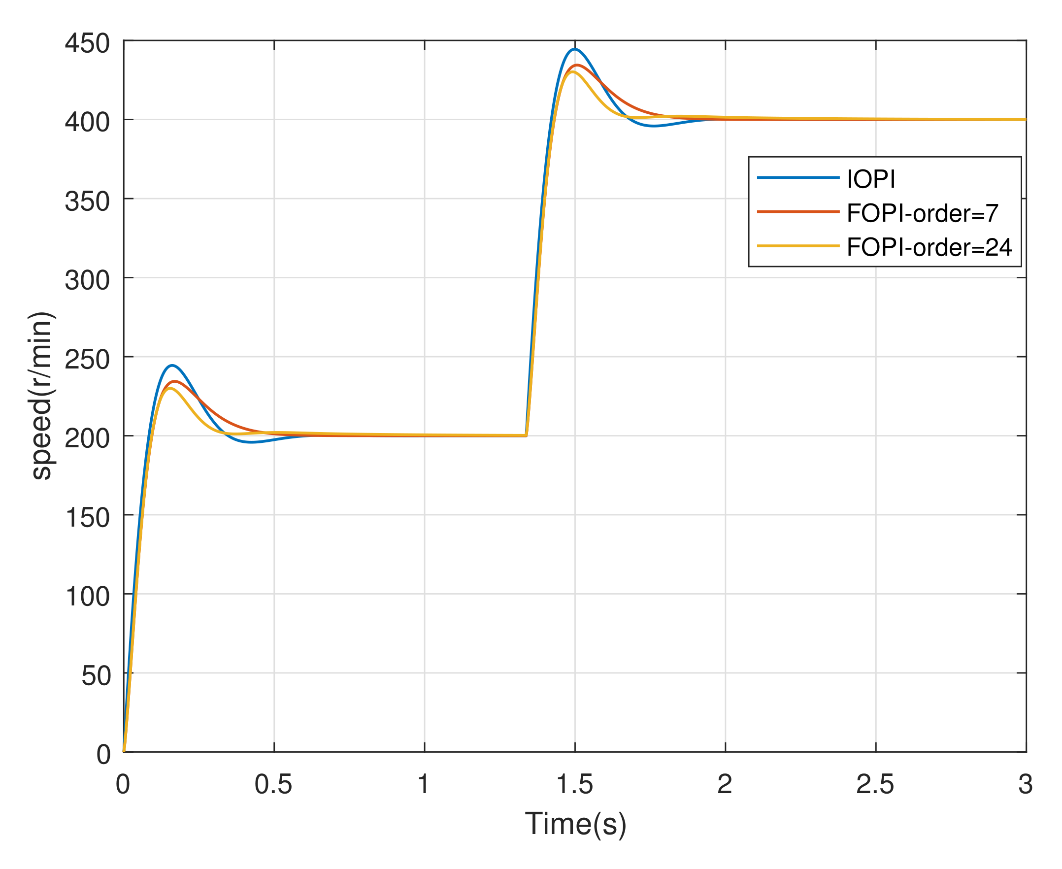
4.2. The Influence of Discretization Order of Impulse Response Invariant Method

The step response waveform is shown in Figure 11, and it can be seen that FOPI has a smaller overshooting and setting time than IOPI. The response of 24th order has a smaller overshoot and smaller setting time than that of 7th order. The comparison of the closed-loop transfer function Bode diagram is shown in Figure 12. The peak value of 24th-order discretization is smaller than that of 7th-order discretization. Therefore, the high-order implementation of the fractional-order operator is more consistent with the expected value and has better performance. In Figure 13, the 24th-order discretization controller input has smaller amplitude oscillations and reaches steady state faster. In Figure 14, the output peak value of the FOPI controller is smaller than the IOPI, and the 24th-order discretization FOPI controller reaches the steady state faster than 7th-order discretization.

The unit step responses of the designed IOPI and FOPI controllers are plotted with controller gain change 0.9 to 1.1 (±10% variations from the nominal value 1), as shown in Figure 15. It can be seen that the designed high-order FOPI controller has a lower overshoot than the IOPI controller. In addition, the overshoots of the high-order FOPI controller remain almost constant under loop gain variations, which means the system is more robust to loop gain changes.

The simulation results of speed reference variations are shown in Figure 16. The speed reference changes from 200 to 400 r/min. Compared with the IOPI controller, the FOPI controller has better dynamic response performance with less overshoot and less adjustment time. In addition, the 24th-order discretization method has better response performance than the 7th-order discretization method.

5. FPGA Design Experimental Verification

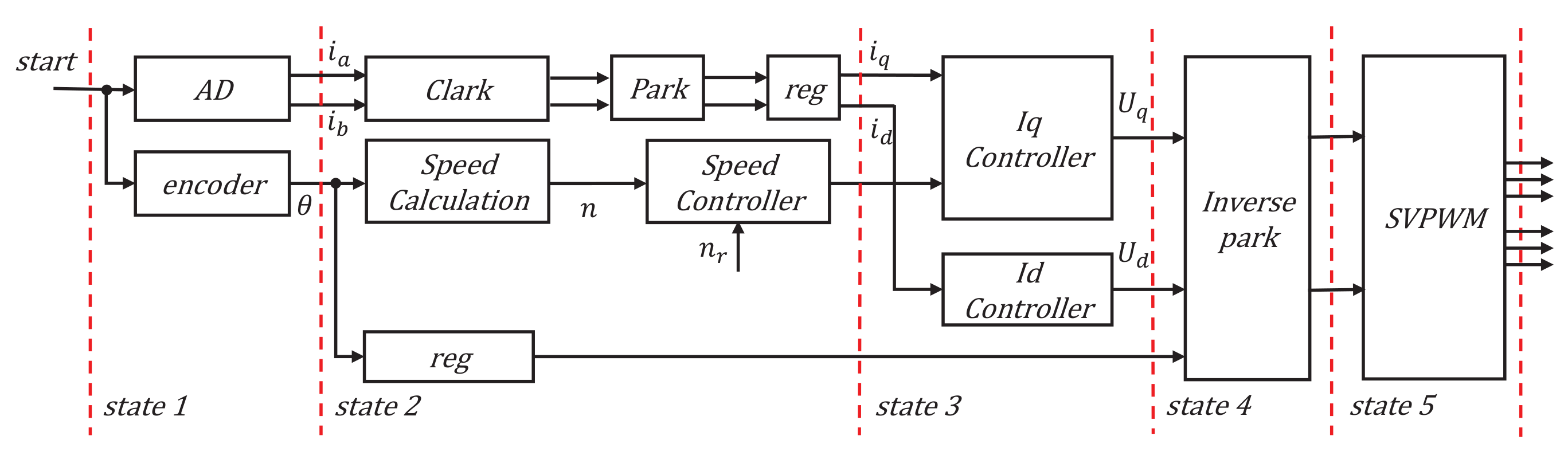
5.1. FOC Algorithm Implementation Based on FPGA

The speed loop control of PMSM is based on the field-oriented control (FOC) method, which decouples the excitation current from the torque current. The FOC structure is shown in Figure 17, where $i_d$ is the d-axis current, $U_d$ is the d-axis voltage, $n_r$ is the reference speed, and $i_a$ and $i_b$ are the two phase currents of the motor. Generally, FOC consists of seven parts: namely, Clark transform, Park transform, inverse Park transform, space vector pulse-width modulation (SVPWM), speed controller, current controller, and speed calculation module. Each part requires a specific computation period, and the longest signal path in each stage determines the bandwidth of this phase. The seven parts together determine the bandwidth of the entire system.

The FOC structure based on FPGA is shown in Figure 18, where $\theta$ is the motor encoder angle value. The whole algorithm process is divided into five states. While the Clark module and the Park module are running, the speed calculation module and the speed controller module can run independently at the same time. Similarly, the $Iq$ controller and the $Id$ controller can operate independently at the same time. Each module makes full use of the FPGA’s concurrent operation to reduce the running time and improve the operation bandwidth. In this paper, the FPGA clock signal is 100 Mhz. Regardless of the current acquisition and encoder acquisition time, the calculation time of the whole speed loop is 127 FPGA clocks.

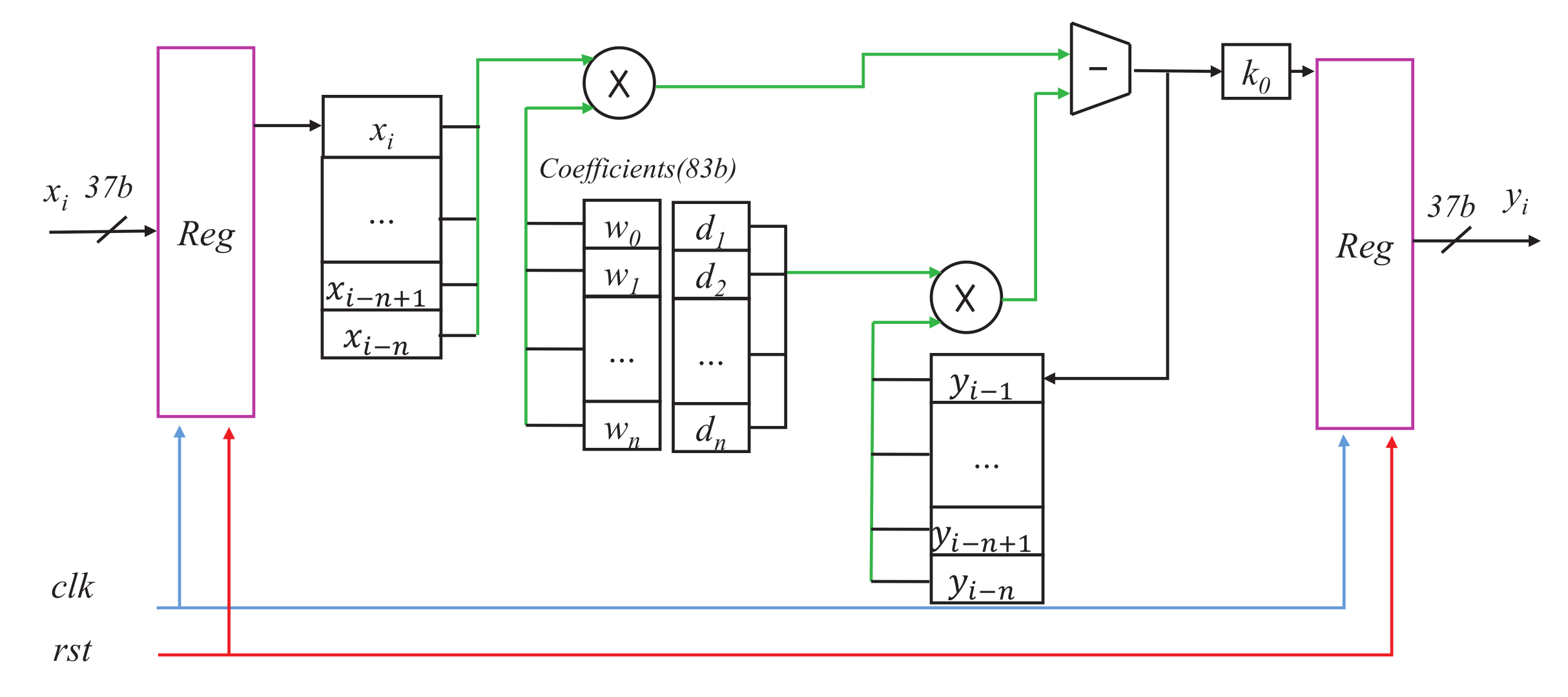
5.2. FPGA Implementation of Fractional-Order Operator

The structure of the fractional PI controller is presented in Figure 17, in which an integrator is connected in series with fractional differential. We study the FPGA implementation of fractional-order operators with reference to FOPI, and the FPGA-based fractional-order operator module can also be used independently for other fractional-order systems. According to the impulse response invariance method, the z-domain expression of the fractional operator $s^{\alpha }$ can be obtained,

$$s^{\alpha }=\frac{NUM}{DEN},$$

(35)

$$NUM=w_0+w_1{z}^{-1}+w_2{z}^{-2}+...+w_n{z}^{-n},$$

(36)

$$DEN=1+d_1{z}^{-1}+d_2{z}^{-2}+...+d_n{z}^{-n},$$

(37)

where $w_i$ and $d_i(i=1...n)$ are the discretization coefficients of fractional-order operators. The fractional differential operator function is as follows,

$$y=x{s}^{\alpha },$$

(38)

where x and y are the input and output. According to Equations (35) and (38), the i-th output can be expressed as

$$y_i=(w_i{x}_i+w_{i-1}{x}_{i-1}+w_{i-2}{x}_{i-2}+...+w_{i-n}{x}_{i-n})-(d_{i-1}{y}_{i-1}+d_{i-2}{y}_{i-2}+...+d_{i-n}{y}_{i-n}).$$

(39)

The hardware implementation of the fractional operator is illustrated in Figure 19. The input and output signals are 37-bit fixed-point numbers, with 5-bits for the integer part and 32-bits for the fractional part. The fractional order operator discretization is an 83-bit fixed-point number, with 13-bits for the integer part and 70-bits for the fractional part. The parameter $k_0$ is the conversion factor, and $k_0$ = $\frac{1}{2^{38}}$. While improving the implementation accuracy of the fractional-order operator, the number of bits of the output signal remains unchanged. Based on the concurrency of FPGA, $w_i{x}_i$ multiplication and $d_{i-1}{y}_{i-1}$ multiplication can be carried out at the same time. While implementing high-precision fractional-order operator, the internal concurrent structure of the module improves the running speed.

The approximate z-domain transfer function of $s^{\alpha }$ ($\alpha$ = 0.5058) is shown as Equations (41)–(43) with the sampling period Ts = 0.00025 s. The integer-order integral operator is discretized using the backward difference method with the same sampling period. When the fractional discretization order is 7,

$$\begin{array}{cc}\hfill NUM=& 71.0130967087276-308.361372264005z^{-1}+544.269486732419z^{-2}\hfill \\ & -498.545074063010z^{-3}+249.992643030789z^{-4}-65.9346494416871z^{-5}\hfill \\ & +7.82911333155244z^{-6}-0.263186494725346z^{-7},\hfill \end{array}$$

(40)

$$\begin{array}{cc}\hfill DEN=& 1-3.73181345431067z^{-1}+5.44679111687348z^{-2}\hfill \\ & -3.86873670327290z^{-3}+1.32371721700043z^{-4}-0.164037126272245z^{-5}\hfill \\ & -0.00750528404544043z^{-6}+0.00161501600045280z^{-7}.\hfill \end{array}$$

(41)

When the fractional discretization order is 24,

$$\begin{array}{cc}\hfill NUM=& 71.0130967087276-284.064316641232z^{-1}+337.351221684772z^{-2}\hfill \\ & -177.279830260836z^{-4}+162.127638162878z^{-8}-191.405704502426z^{-10}\hfill \\ & +106.826515785161z^{-12}-40.3918077785183z^{-15}+22.7466788382580z^{-17}\hfill \\ & -12.7261323351444z^{-19}+7.48334445354109z^{-20}-1.89892481499192z^{-21}\hfill \\ & +0.229665363193541z^{-22}-0.0115954062078416z^{-23}+0.000150746521401462z^{-24},\hfill \end{array}$$

(42)

$$\begin{array}{cc}\hfill & DEN=1-3.38966451631363z^{-1}+2.74186995466488z^{-2}\hfill \\ & +1.52114228620950z^{-3}-1.54865386366973z^{-4}-0.794250251335307z^{-5}\hfill \\ & -0.470762396086378z^{-6}-0.350412508116731z^{-7}+1.99620214850720z^{-8}\hfill \\ & +1.14667011512325z^{-9}-1.92550294458525z^{-10}-1.03508909072953z^{-11}\hfill \\ & +0.854840960387078z^{-12}+0.420251295731053z^{-13}+0.236729664910028z^{-14}\hfill \\ & -0.397330340171471z^{-15}-0.209087294971177z^{-16}+0.191654930415509z^{-17}\hfill \\ & +0.0979007198034854z^{-18}-0.121300895228491z^{-19}+0.0392770038980040z^{-20}\hfill \\ & -0.00442457810491528z^{-21}-0.000100857599349359z^{-22}+4.17152916747670e-05z^{-23}\hfill \\ & -1.25464323233953e-06z^{-24}.\hfill \end{array}$$

(43)

5.3. Experimental Verification

The experimental platform is shown in Figure 20, including a PMSM, servo driver, and PC interface. The servo drive is based on FPGA-10M50DAF484C7G, which is used for encoder reading, AD sampling, and control algorithm implementation. The FPGA-10M50DAF484C7G has 484 pins and 50K logic elements, and the maximum frequency is 450 MHz. The motor is VM7-M13A-2R020-D1, and the parameters are shown in

Table 2. Parameters of PMSM.

Motor Parameters	Value	Unit
Rated power	2.0	kW
Rated speed	2000	r/min
Rated voltage	220	V
Rated current	9.1	A

.

The speed responses of the FOPI and IOPI are shown in Figure 21. The discretization order 24th step response has a smaller overshoot and adjustment time. For a fair comparison, the controllers gain are set as 90%, 100%, and 110% of the nominal value. As shown in Figure 22 and Figure 23, the high-order fractional order controller achieves better robustness.

Figure 24 shows that the FOPI controller has better dynamic response performance than the IOPI controller when speed changes. In addition, the 24th-order discretization method based on FPGA implementation has better response performance than the 7th-order discretization method.

6. Conclusions

In this paper, an FOPI controller is designed to control the speed of PMSM, and the numerical implementation accuracy of the fractional-order operator is investigated. Three common numerical implementation methods of the fractional-order operator are studied. Both the impulse response invariant method and the Oustaloup method have good fitting performance with 24th-order discretization. The effects of different discretization orders with the impulse response invariant method on the control performance of the system are compared. The FOC algorithm is implemented based on very high speed integrated circuit hardware description language (VHDL), including the IOPI controller and high-performance FOPI controller. Compared with the traditional pipelined structure microprocessor, FPGA can break through the limitation of data bits, and the parallel characteristic can improve the running speed. According to the simulation and experimental results of the PMSM speed loop, the servo system based on the high-order FOPI controller can obtain better dynamic response performance and robustness. The FPGA-based fractional-order operator module can be integrated into other fractional-order systems.

References

1. Machado, J. Analysis and design of fractional-order digital control systems. Syst. Anal. Model. Simul. 1997, 27, 107–122. [Google Scholar]
2. Vinagre, B.M.; Petras, I.; Merchan, P.; Dorcak, L. Two digital realization of fractional controllers: Application to temperature control of a solid. In Proceedings of the 2001 European Control Conference (ECC), Porto, Portugal, 4–7 September 2001; pp. 1764–1767. [Google Scholar]
3. Luo, Y.; Wang, C.Y.; Chen, Y. Tuning fractional order proportional integral controllers for fractional order systems. J. Process. Control 2010, 20, 823–831. [Google Scholar] [CrossRef]
4. Wang, X.; He, Y. Projective synchronization of fractional order chaotic system based on linear separation. Acta Phys. Sin. 2007, 372, 435–441. [Google Scholar] [CrossRef]
5. Abdelaty, A.M.; Roshdy, M.; Said, L.A.; Radwan, A.G. Numerical Simulations and FPGA Implementations of Fractional-Order Systems Based on Product Integration Rules. IEEE Access 2020, 8, 102093–102105. [Google Scholar] [CrossRef]
6. Engheta, N. Fractional calculus and fractional paradigm in electromagnetic theory. In Proceedings of the MMET Conference Proceedings, 1998 International Conference on Mathematical Methods in Electromagnetic Theory, MMET 98 (Cat. No.98EX114), Kharkov, Ukraine, 2–5 June 1998; pp. 879–880. [Google Scholar]
7. Fogang, C.; Pelap, F.; Tanekou, G.B.; Kengne, R.; Fidèle, K. Earthquake dynamic induced by the magma up flow with fractional power law and fractional-order friction. Ann. Geophys. 2021, 64, SE101. [Google Scholar] [CrossRef]
8. Li, H.S.; Luo, Y.; Chen, Y.Q. A fractional order proportional and derivative (FOPD) motion controller: Tuning rule and experiments. IEEE Trans. Control Syst. Technol. 2010, 18, 516–520. [Google Scholar] [CrossRef]
9. Shi, L.; Gao, S.; Xi, H.; Yuan, H.; Zhou, T. FPGA realization of a speech encryption system based on a generalized modified chaotic transition map and bit permutation. Multimed. Tools Appl. 2019, 78, 16097–16127. [Google Scholar]
10. Sabatini, V.; Benedetto, M.D.; Lidozzi, A. Synchronous Adaptive Resolver-to-Digital Converter for FPGA-Based High-Performance Control Loops. IEEE Trans. Instrum. Meas. 2019, 68, 3972–3982. [Google Scholar] [CrossRef]
11. Romero-Troncoso, R.J.; Saucedo-Gallaga, R.; Cabal-Yepez, E.; Garcia-Perez, A.; Osornio-Rios, R.A.; Alvarez-Salas, R.; Mir a-Vidales, H.; Huber, N. FPGA-based online detection of multiple combined faults in induction motors through information entropy and fuzzy inference. IEEE Trans. Ind. Electron. 2011, 58, 5263–5270. [Google Scholar] [CrossRef]
12. Gulbudak, O.; Santi, E. FPGA-Based Model Predictive Controller for Direct Matrix Converter. IEEE Trans. Ind. Electron. 2016, 63, 4560–4570. [Google Scholar] [CrossRef]
13. Kung, Y.; Tseng, K.; Tai, T. FPGA-based Servo Control IC for X-Y Table. In Proceedings of the 2006 IEEE International Conference on Industrial Technology, Mumbai, India, 15–17 December 2006; pp. 2913–2918. [Google Scholar]
14. Cho, J.U.; Le, Q.N.; Jeon, J.W. An FPGA-based multiple-axis motion control chip. IEEE Trans. Ind. Electron. 2009, 56, 856–870. [Google Scholar]
15. Rovere, L.; Formentini, A.; Zanchetta, P. FPGA Implementation of a Novel Oversampling Deadbeat Controller for PMSM Drives. IEEE Trans. Ind. Electron. 2019, 66, 3731–3741. [Google Scholar] [CrossRef]
16. Chen, Z.; Zhang, H.; Tu, W.; Tan, B.; Luo, G. FPGA Implementation of an Arbitrary Injection based Sensorless Control for PMSM. In Proceedings of the 2018 IEEE Energy Conversion Congress and Exposition (ECCE), Portland, OR, USA, 23–27 September 2018; pp. 1741–1747. [Google Scholar]
17. Xu, Y.; Shuang, K.; Jiang, S.; Wu, X. FPGA implementation of a best-precision fixed-point digital PID controller. In Proceedings of the 2009 International Conference on Measuring Technology and Mechatronics Automation, Zhangjiajie, China, 11–12 April 2009; pp. 384–387. [Google Scholar]
18. Jatoth, R.K.; Rajasekhar, A. Adaptive bacterial foraging optimization based tuning of optimal PI speed controller for PMSM drive. Int. Conf. Contemp. Comput. 2010, 94, 588–599. [Google Scholar]
19. Chen, P.C.; Luo, Y.; Zheng, W.J.; Gao, Z.; Chen, Y.Q. Fractional order active disturbance rejection control with the idea of cascaded fractional order integrator equivalence. ISA Trans. 2020, 114, 1879–2022. [Google Scholar] [CrossRef]
20. Zheng, W.J.; Luo, Y.; Wang, X.H.; Pi, Y.G.; Chen, Y.Q. Fractional order PID controller design for satisfying time and frequency domain specifications simultaneously. ISA Trans. 2017, 68, 212–222. [Google Scholar] [CrossRef]
21. Zaihidee, F.M.; Mekhilef, S.; Mubin, M. Fractional order PID sliding mode control for speed regulation of permanent magnet synchronous motor. Nonlinear Dyn. 2021, 9, 209–218. [Google Scholar] [CrossRef]
22. Chen, P.; Luo, Y.; Peng, Y.; Chen, Y. Optimal Fractional-Order Active Disturbance Rejection Controller Design for PMSM Speed Servo System. Entropy 2021, 23, 262. [Google Scholar] [CrossRef]
23. Chopade, A.S.; Khubalkar, S.W.; Junghare, A.S.; Aware, M.V.; Das, S. Design and implementation of digital fractional order pid controller using optimal pole-zero approximation method for magnetic levitation system. IEEE/CAA J. Autom. Sin. 2018, 5, 977–989. [Google Scholar] [CrossRef]
24. Tolba, M.F.; Said, L.A.; Madian, A.H.; Radwan, A.G. FPGA implementation of fractional-order integrator and differentiator based on Grünwald Letnikov’s definition. In Proceedings of the 2017 29th International Conference on Microelectronics (ICM), Beirut, Lebanon, 10–13 December 2017; Volume 78, pp. 1–4. [Google Scholar]
25. Tolba, M.F.; AboAlNaga, B.M.; Said, L.A.; Madian, A.H.; Radwan, A.G. Fractional order integrator/differentiator: FPGA implementation and FOPID controller application. AEU-Int. J. Electron. Commun. 2019, 98, 220–229. [Google Scholar] [CrossRef]
26. Tolba, M.F.; Saleh, H.; Mohammad, B. Enhanced FPGA realization of the fractional-order derivative and application to a variable-order chaotic system. Nonlinear Dyn. 2020, 99, 3143–3154. [Google Scholar] [CrossRef]
27. Poinot, T.; Trigeassou, J.C. Identification of fractional systems using an output-error technique. Nonlinear Dyn. 2004, 38, 133–154. [Google Scholar] [CrossRef]
28. Luo, Y.; Chen, Y.Q. Fractional Order Motion Controls; John Wiley Sons Ltd.: Hoboken, NJ, USA, 2013; pp. 1–24. [Google Scholar]
29. Tolba, M.F.; AbdelAty, A.M.; Said, L.A.; Ahmed, S.; Elwakil, A.T.A.; Madian, A.H.; Ounnas, A.; Radwan, A.G. FPGA realization of Caputo and Grünwald-Letnikov operators. In Proceedings of the 2017 6th International Conference on Modern Circuits and Systems Technologies (MOCAST), Thessaloniki, Greece, 4–6 May 2017; pp. 1–4. [Google Scholar]
30. Podlubny, I. Fractional Differential Equations: An Introduction to Fractional Derivatives, Fractional Differential Equations, to Methods of Their Solution and Some of Their Applications; Elsevier: Amsterdam, The Netherlands, 1999; pp. 41–119. [Google Scholar]
31. Tolba, M.F.; Said, L.A.; Madian, A.H.; Radwan, A.G. FPGA Implementation of the Fractional Order Integrator/Differentiator: Two Approaches and Applications. IEEE Trans. Circuits Syst. I Regul. Pap. 2019, 66, 1484–1495. [Google Scholar] [CrossRef]
32. Ferdi, Y. Computation of fractional order derivative and integral via power series expansion and signal modelling. Nonlinear Dyn. 2006, 46, 1–15. [Google Scholar] [CrossRef]
33. Chen, Y.; Vinagre, B.M.; Podlubny, I. Continued fraction expansion approaches to discretizing fractional order derivatives—An expository review. Nonlinear Dyn. 2004, 38, 155–170. [Google Scholar] [CrossRef]
34. Oustaloup, A.; Levron, F.; Mathieu, B.; Nanot, F.M. Frequency-band complex noninteger differentiator: Characterization and synthesis. IEEE Trans. Circuits Syst. I Fundam Theory Appl. 2000, 47, 25–39. [Google Scholar] [CrossRef]
35. Carlson, G.; Halijak, C. Approximation of fractional capacitors by a regular Newton process. IEEE Trans. Circuit Theory 1964, CT-11, 210–213. [Google Scholar] [CrossRef]
36. Impulse Response Invariant Discretization of Fractional Order Integrators/Dierentiators. Available online: http://www.mathworks.com/matlabcentral/fileexchange/21342-impulse-response-invariant-discretization-of-fractional-order-integrators-dierentiators (accessed on 1 September 2020).
Figure 1. The research workflow of this paper.
Fractalfract 06 00218 g001
Figure 2. The PMSM speed control system.
Fractalfract 06 00218 g002
Figure 3. Open−loop Bode plot with the different controllers.
Fractalfract 06 00218 g003
Figure 4. 7th−order discretization approximate Bode graph of s 0.5 in the frequency band [0.01, 1000] Hz.
Fractalfract 06 00218 g004
Figure 5. 24th−order discretization approximate Bode graph of s 0.5 in the frequency band [0.01, 1000] Hz.
Fractalfract 06 00218 g005
Figure 6. 24th−order discretization approximate Bode graph of s 0.5 in the frequency band [0.01, 10,000] Hz.
Fractalfract 06 00218 g006
Figure 7. 24th−order discretization approximate Bode graph of s 0.1 in the frequency band [0.01, 1000] Hz.
Fractalfract 06 00218 g007
Figure 8. 24th−order discretization approximate Bode graph of s 0.9 in the frequency band [0.01, 1000] Hz.
Fractalfract 06 00218 g008
Figure 9. Bode plot of fractional order operator s 0.5058 .
Fractalfract 06 00218 g009
Figure 10. Open−loop Bode plot with the different controllers.
Fractalfract 06 00218 g010
Figure 11. Speed response comparison with different controllers.
Fractalfract 06 00218 g011
Figure 12. Closed−loop Bode plot with different discretization orders.
Fractalfract 06 00218 g012
Figure 13. The controllers input signals.
Fractalfract 06 00218 g013
Figure 14. The controllers output signals.
Fractalfract 06 00218 g014
Figure 15. Step responses with loop gain variations.
Fractalfract 06 00218 g015
Figure 16. Speed variations response.
Fractalfract 06 00218 g016
Figure 17. FOC algorithm.
Fractalfract 06 00218 g017
Figure 18. FOC algorithm control based on FPGA.
Fractalfract 06 00218 g018
Figure 19. The hardware architecture of fractional operator.
Fractalfract 06 00218 g019
Figure 20. The experimental platform.
Fractalfract 06 00218 g020
Figure 21. PMSM speed step response (Experiment).
Fractalfract 06 00218 g021
Figure 22. The speed responses of the PMSM system with different IOPI controller gains (Experiment).
Fractalfract 06 00218 g022
Figure 23. The speed responses of the PMSM system with different FOPI controller gains (Experiment).
Fractalfract 06 00218 g023
Figure 24. Speed variations response (Experiment).
Fractalfract 06 00218 g024