1. Introduction
The development of graphics technology and applications generates a huge number of images carrying valuable information, such as medical examination results, traffic condition diagrams and remote sensing images [
1]. The wide range of graphics causes the problem that the vagueness of images will lead to information leakage and even misguidedness [
2]. Under these circumstances, image enhancement methods are of great significance to highlight necessary information.
Image segmentation is a critical step before the enhancement process because of its ability to gather similar regions. Numerous image segmentation algorithms have been introduced in recent years based on different properties, such as rough set theory [
3,
4,
5], genetic algorithms [
6,
7,
8] and fuzzy set theory [
9,
10,
11]. Furthermore, the image segmentation algorithms can be divided into several types, such as region-based algorithms, edge detection algorithms and clustering algorithms. These algorithms keep innovating on the original basis to seek a better segmentation effect. However, while these algorithms have been demonstrated to be an effective tool to handle uncertain or incomplete information, they still have the problems of missing detailed information, instability and introducing unrelated information in segmentation results. In this article, a new image segmentation algorithm based on roughness is proposed, which not only considers the difference in image regions but also uses similarity with neighbor pixels to cluster difference image patterns, combining the advantages of region-based and clustering algorithms. The preprocessed results show that this algorithm has more segmentation outputs and preserves more details and the patterns in each layer share higher similarity.
The quality of an image is enhanced through successive applications such as histogram manipulation [
12], gamma correction [
13] and contrast stretching [
14]. While these methods have improved the image quality to some extent, they have their restrictions. For example, histogram-based methods are suitable for images that only have one peak in their histograms. Furthermore, these methods may not highlight necessary information as they are applied on the whole image without considering the gradient of the gray level. The digital fractional order differentiator is an effective tool to deal with these problems and has good stability in image enhancement. Recently, the interest in image enhancement techniques based on a fractional differential operator mask has grown in the field of image processing. Liu et al. [
15] introduced the fractional differential wavelet algorithm which can greatly improve the high-frequency components of the signal and the very low frequency of the nonlinear retained signal. Kaur et al. [
16] proposed a technique based on the Riesz fractional derivative in the fractional Fourier transform domain that outperformed the existing techniques by providing improvement in various performance parameters. Singh et al. [
17] employed a piecewise gamma corrected fractional differential order masking framework for image quality enhancement. Experiments showed that the proposed approach had advantages compared with the conventional and state-of-the-art nonreal time algorithms. While these algorithms showed improvement, they still had problems of instability and cannot manage different kinds of information. Aiming at solving these problems, this paper proposes a new algorithm based on rough set theory and a fractional order differential operator.
The core contributions of the paper to achieve higher enhancement quality are identified as follows:
A new image segmentation algorithm based on rough set theory and a Gaussian mixture model is proposed, which combines the advantage of addressing uncertain boundaries and centralizing similar information from rough set theory and the property of clustering from a Gaussian mixture model.
We use 2D Fourier transform to change the gray level to image gradient and use filters to preserve different types of information. By applying a four-direction fractional differential mask on the Fourier domain, the proposed algorithm not only prevents the blur and shadow that could happen but also achieves the best enhancement for different types of frequency.
Entropy is employed as a cost function to calculate the optimal fractional order to preserve more image information and avoid degradation, which makes the enhanced images more suitable for computer vision processing.
The rest of the paper is organized as follows:
Section 2 introduces the background knowledge of the proposed algorithm.
Section 3 shows the detailed process of image segmentation and enhancement.
Section 4 lists the experimental results to verify the performance and effectiveness.
Section 5 concludes the whole paper.
2. Preliminary
In the image segmentation process, rough set theory is used to search for similar pixel points while a Gaussian mixture model is employed to cluster gray levels. After segmentation, Fourier transform is used to turn gray levels into frequency, then a fractional order differential operator is employed to enhance 2D signals in the image enhancement process.
2.1. Rough Set Theory
The rough set theory, first introduced by Pawlak in 1982 [
18], has been proved to be an efficient analysis algorithm for studying uncertain information and incomplete data. It is effective in mining potential relationships between items without the need for additional relevant information.
For a given nonempty set
U with limited elements
,
R is an equivalent relation on
U and
indicates the set of all the elements that are indistinguishable from
under
R. When
X cannot be precisely described by the attribute of
R,
X is an undefined set or rough set of
R. The
R-lower and
R-upper approximations of set
X are defined as the following, respectively
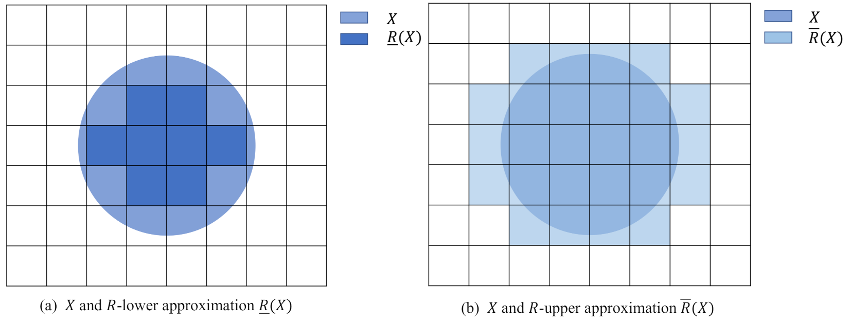
One example of the relationship between
R-upper and
R-lower approximations of set
X and
X is shown in
Figure 1.
Then, the
R-upper and
R-lower approximations have the following properties:
The boundary region in rough set theory is . If the R-upper and the R-lower approximations are identical, i.e., , then the set X is called an exact set.
The roughness of the set is caused by the boundary region. The larger the boundary region is, the less accurate set
X is. In order to express this relationship, the measure of roughness is defined as
The roughness measure can reflect the uncertainty of set
X. For example, in
Figure 1, the roughness measure of set
X is
.
2.2. Gaussian Mixture Model
A Gaussian model is a common variable distribution model which is widely used in the field of mathematical statistics. The probability density function of a 1D Gaussian distribution is defined as follows:
where
,
and
represent expectation and variance, respectively.
A Gaussian mixture model (GMM) [
19] is regarded as a model composed of several Gaussian models, which are hidden variables of the GMM. The GMM can be used to smoothly approximate any given curve.
The probability density distribution of the GMM is
where
x is the observed data,
K is the number of Gaussian models,
is the component proportion of the
kth model and
.
An example of a GMM of three Gaussian models with component
is shown in
Figure 2.
The hidden variables and of the GMM are needed to approximate a given curve. In this paper, an expectation maximum algorithm is employed to calculate the hidden variables. After building the GMM, intensity g is clustered by assigning it to the class with the largest posterior probability.
2.3. Fourier Transform
Fourier transform has been considered as a classical signal processing algorithm and one of the most critical analytical tools in many fields. Fourier transform can turn a square integrable function into a combination of circular functions. This algorithm can be used to transform the signal between the space and frequency domain.
In image processing, as the distribution function of an image is not continuous, 2D Fourier transform needs to be discretized. For an
image, the discrete 2D Fourier transform and its inverse transform are defined as:
where
is the distribution of the image gradient. The bright or dark parts on the
represent the value of the gradient. If the gradient is large, then the brightness on
is high, otherwise it is low. The energy distribution of the image can be obtained by observing
. After shifting
to the origin, a conclusion can be drawn that the frequency is symmetrically distributed. The 2D Fourier transform of image “3.2.25” from the USC-SIPI image database “Aerials” and its shifted frequency image are shown in
Figure 3.
2.4. Fractional Differential Operator
Fractional differentiation is the broad sense of integer-order differentiation and includes the
nth derivative as a particular case [
20,
21]. There are three classical definitions of a fractional differentiator, the Grünwald–Letnikov definition, the Riemann–Liouville definition and the Caputo definition [
22]. This paper uses the Gr
nwald–Letnikov fractional derivative definition as it has the advantages of being able to convert to convolution in numerical implementation and is suitable for image signal processing. For 1D signal
, the definition of the Gr
nwald–Letnikov fractional differentiator of order
is
According to Equation (
11), if the period is divided by
,
. Then, the fractional differential expression is obtained [
23]:
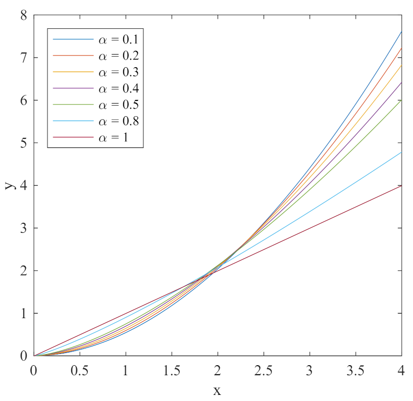
Under the definition of Gr
nwald–Letnikov, the fractional differential of
for different orders
is shown in
Figure 4.
For an
image
f, as the gray level is finite, the largest variance is bounded. Furthermore, considering the discreteness of the image, the minimum interval in
is the distance between adjacent pixels, which means
. Then, in the
x and
y direction,
n is
,
, respectively. For image
f, the fractional differential is defined as follows in the
x and
y direction:
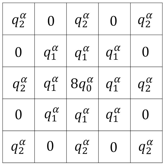
Then, a four-direction fractional order differentiator mask can be built as shown in
Figure 5.
This paper employs the four-direction fractional order differentiator mask to scan the 2D transformed image gradient. Then, Fourier inverse transform is used to obtain the enhanced image.
3. Proposed Methodology
3.1. Image Segmentation Algorithm
The intention of the segmentation algorithm is to produce image layers containing similar pixels, which can avoid burrs later in the image enhancement process. The rough set approach is employed to find pixels similar to the neighborhood while a Gaussian mixture model is used to cluster gray levels into several categories.
3.1.1. Histogram and Histon
Let
f be the original
image, then the histogram is calculated by
where
is the unit impulse function and
L denotes the largest gray level.
Considering the
neighborhood around pixel
, the total distance between all the pixels in the neighborhood and
is calculated by
By setting a threshold
, the matrix
X of size
is built by
Then, the pixels in the neighborhood are assumed to be similar to pixel if and their similarity decreases exponentially when .
Taking the discrepancy between distributions in different regions into consideration, the threshold
is supposed to be larger for small regions to expand the
R-upper approximation of the histogram,
where
k is the threshold of proportion of pixel intensity
g. In this article, we set
,
and
.
Then, the histon [
24] is defined as
The histogram and histon of the origin image are considered as the R-lower approximation and R-upper approximation in the rough set theory, respectively. The histogram value represents the number of pixels in the set of the gth gray level while the histon value of the gth gray level represents the number of all the pixels considered similar to g.
We substitute the histogram and histon into Equations (
3)–(
5). We can see the value of histograms will always be smaller than the histon. Furthermore, the histogram and histon value of gray level
and
will be the sum of their corresponding value. Then, it is verified that the histogram and histon satisfy all the properties in the rough set theory, which means they can be seen as the
R-lower approximation and
R-upper approximation.
3.1.2. Cluster Based on Gaussian Mixture Model
According to the rough set theory, the roughness measure is defined as
However, the definition of histogram and histon determines their discreteness, which means the roughness measure function is discontinuous and it is difficult to separate its peaks and valleys. Under this circumstance, instead of using the function, this paper uses the Gaussian kernel function to smooth the histogram and histon. Then, a Gaussian mixture model is applied to fit the roughness measure function.
The probability density distribution of the roughness measure function is
where
represents the component proportion of each Gaussian model,
and
K are chosen by cross validation. For every given gray level
g, it is assigned to the component Gaussian model yielding the highest posterior probability.
The segmentation process is described as follows:
- Step 1:
For an
image
f, for every channel, calculate its histogram
by using Equation (
15).
- Step 2:
Use histogram
to consider the
gth gray level as a small or large region and assign the corresponding threshold by Equation (
18).
- Step 3:
Calculate the
weight matrix
X by using Equation (
17).
- Step 4:
Calculate the histon
by using Equation (
19).
- Step 5:
Use the Gaussian kernel function to smooth
and
and calculate the rough measure function
with Equation (
20).
- Step 6:
Use a Gaussian mixture model to fit the rough measure model and cluster the gray level.
- Step 7:
Use the cluster result to segment image f and obtain a series of segmentation results S.
The segmentation layers of image “3.2.25” are shown in
Figure 6.
The segmentation method proposed in the paper combined the rough set measure with the Gaussian mixture model. Compared with traditional segmentation methods which only divide an image into the object and background, this method has more segmentation layers which will preserve more details and pixels in every layer sharing higher similarity.
3.2. Adaptive Fractional Order Differential Mask for Image Enhancement in Fourier Domain
After preprocessing segmentation layers, this paper first uses 2D Fourier transform to turn gray levels into an image gradient, then applies filters to extract and enhance boundary and base information, respectively. Finally, a four-direction adaptive fractional differential mask based on entropy is employed to enhance images.
3.2.1. Preprocess
As the range of gray levels in segmentation layers might be wide, we compress the segmentation results
S by using a logarithmic function. Then, to avoid burrs in the image enhancement process, blank regions are filled artificially in each segmentation layer with average nonzero pixel intensity by
where
is the image to be enhanced,
is the compressed segmentation results,
. The comparison of preprocessed images of the third layers of image “3.2.25” is shown in
Figure 7. It can be seen that the pixels in the final preprocessed image are all in a small range of gray level and there are few adjacent regions with large variance.
3.2.2. Adaptive Fractional Differential-Based Image Enhancement Process in Fourier Domain
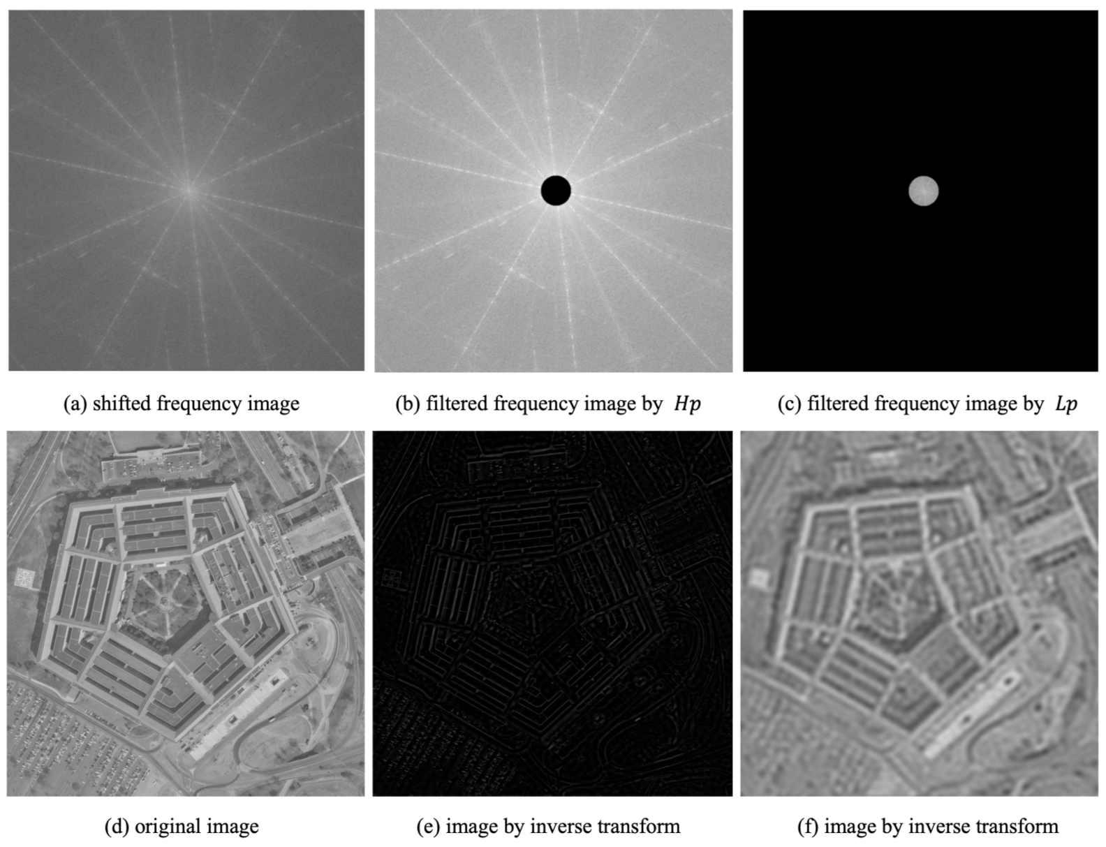
Then, the frequency images are obtained by 2D Fourier transform. By setting threshold , a high-pass filter () and low-pass filter () are obtained to extract the boundary details and basic information of the image.
Let , , and . In an Fourier frequency image, reserves the points with while reserves the points with .
The Fourier frequency images of the filtered images by
and
and their inverse transform results are shown in
Figure 8.
Considering that the choice of fractional order will affect the image enhancement performance, this paper uses an unsupervised optimization algorithm to find the optimal fractional order. The concept of information entropy [
25] is introduced to measure the distribution of gray value in an image to calculate the optimal parameter. The higher the value of entropy is, the more information the image transports. The formula of information entropy is
where
is the frequency of the
gth gray level and
L denotes the largest gray level of image
f. After obtaining the optimal fractional order parameter, a fractional mask is used to enhance the image.
The image enhancement process is described as follows:
- Step 1:
Use a segmentation method above to obtain a series of image layers.
- Step 2:
Calculate the and filters to extract the boundary and fundamental information.
- Step 3:
Calculate the optimal fractional order parameter for filtered images and based on maximizing the entropy of and .
- Step 4:
Apply a fractional order differentiator mask on the enhanced filtered images and , respectively.
- Step 5:
Combine the enhanced results.
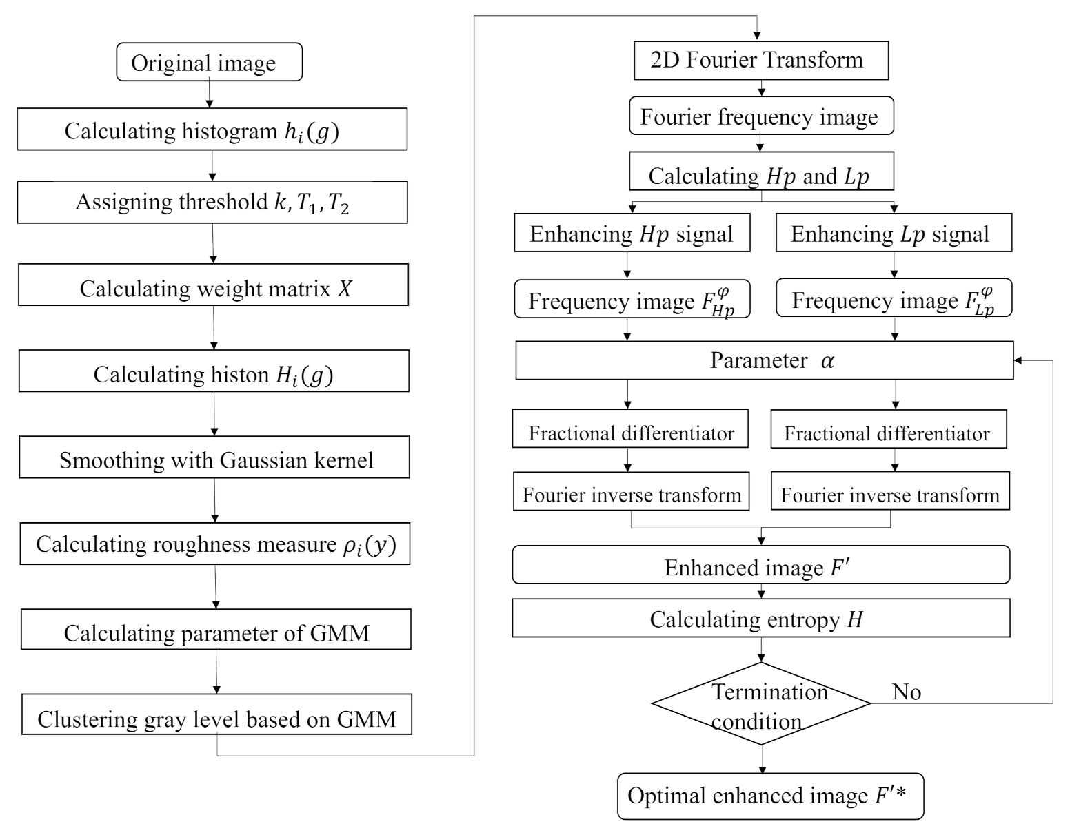
The block diagram of proposed algorithm is shown in
Figure 9.
4. Experimental Results and Numerical Analysis
4.1. Experimental Results
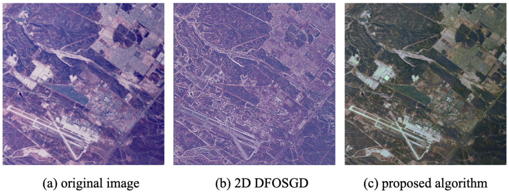
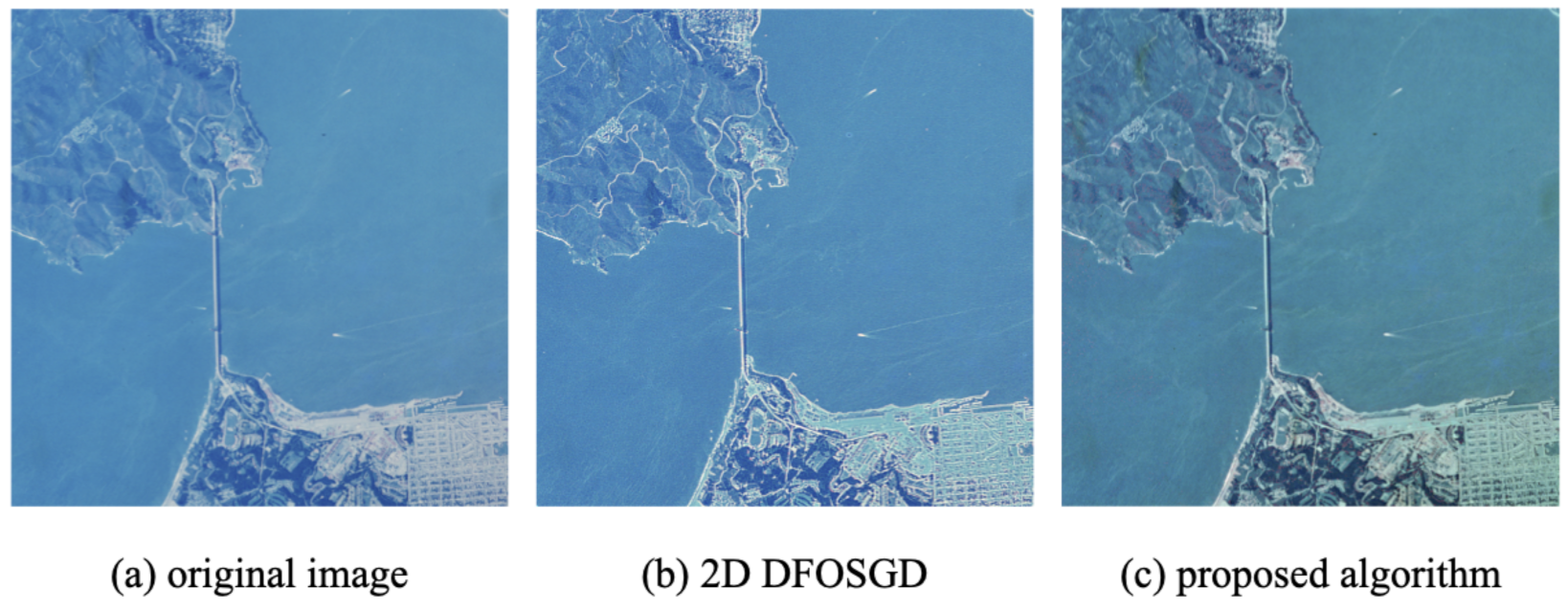
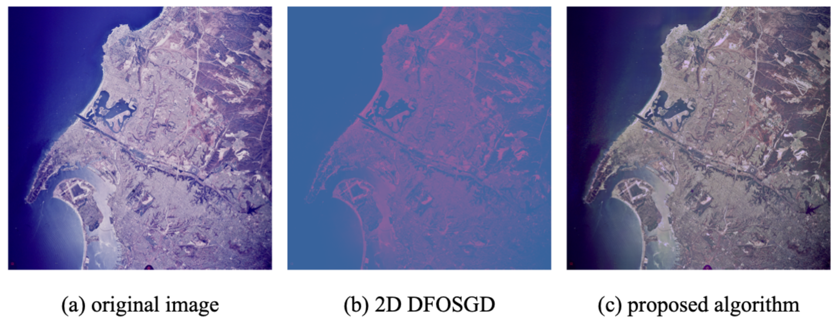
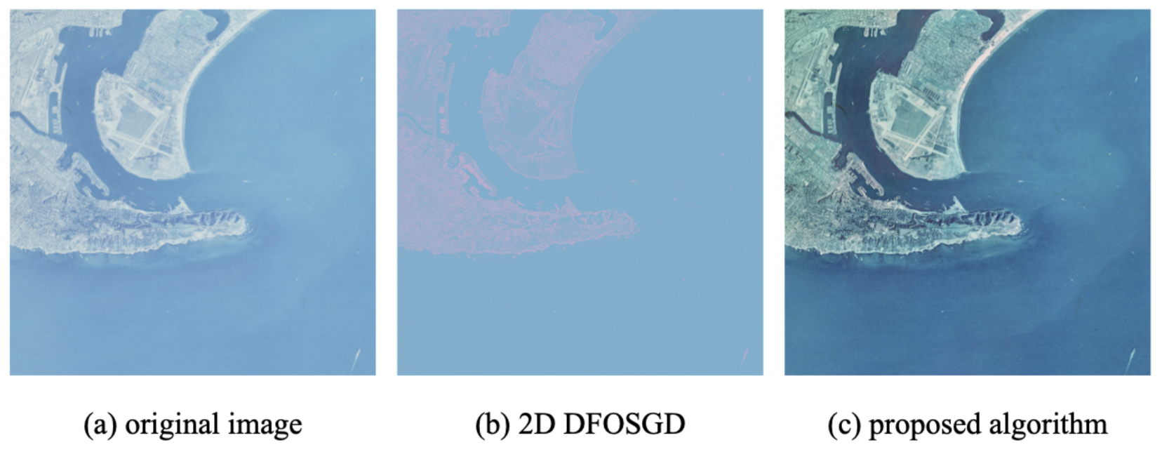
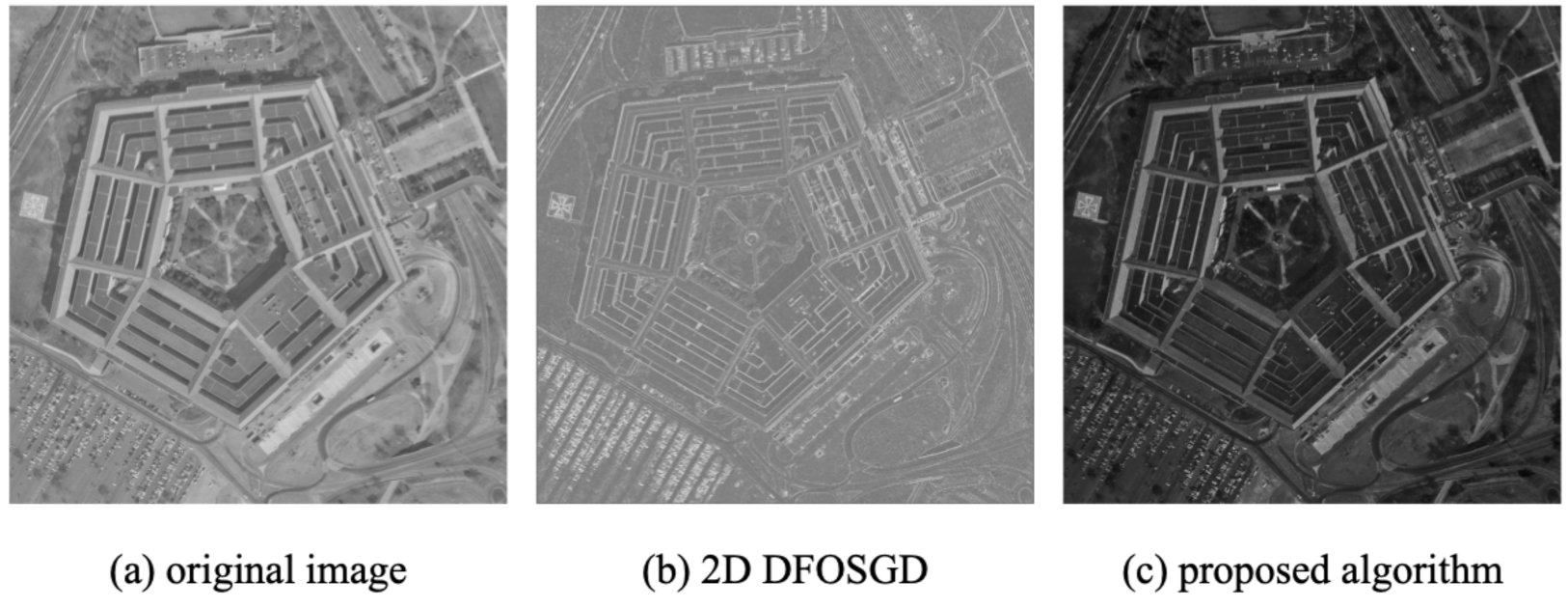
In order to verify the image enhancement performance, we apply the algorithm on the USC-SIPI image database “Aerials”, which was distributed in 1977 and consists of 37 color and one monochrome high-altitude aerial images, and list the enhanced results of the proposed method for six images (
https://sipi.usc.edu/database/database.php?volume=aerials, accessed on 25 February 2022). The image enhancement performance of this method is compared with that of the 2-D DFOSGD method [
26], which also builds an adaptive fractional order differentiator enhancement model. The comparison results are listed in
Figure 10,
Figure 11,
Figure 12,
Figure 13,
Figure 14 and
Figure 15.
It is noted that compared with the original images, the proposed algorithm shows good enhancement results. Apart from this, the proposed algorithm extracts more texture details and makes the unobtrusive pattern more observable than the algorithm in [
26].
4.2. Numerical Analysis
To further prove the efficiency of the proposed algorithm, a series of numerical analyses has been carried out with classical image enhancement algorithms such as 2D DFOSGD [
26], LIME [
27], Dong [
28], MSRCP [
29] and MSRCR [
29].
4.2.1. Information Entropy Analysis
Shannon’s information theory introduces the concept of information entropy and uses it to measure the distribution of gray values of an image. As this paper uses the model based on an entropy adaptive model to choose fractional order and, in the other algorithms, we use the same process to choose optimal to carry out the comparison experiments.
The comparison of the information entropy of enhanced images is shown in
Table 1. The experimental results show that the entropy of the images enhanced by the proposed scheme is larger than that of the others, which means they can provide more information for later computer vision processing.
4.2.2. Peak Signal to Noise Ratio
Peak signal to noise ratio (PSNR) measures the quality between the original image and the enhanced image. A higher PSNR value indicates less degradation of the image. It is estimated by calculating the value of mean square error (MSE) as
As the PSNR is the measure for gray images, in the experiment we average the gray level of the three channels of original and enhanced images as inputs to calculate MSE and PSNR. The comparison of PSNR of enhanced images is shown in
Table 2.
By analyzing the comparable results from
Table 2, we find that the results of the proposed algorithm are better than most existing algorithms. Some results are smaller because the proposed algorithm emphasizes more interesting regions. While the information is preserved, the difference in gray level increases, which will increase the value of MSE.
4.2.3. Structural Similarity
To have a better understanding of the degradation of the image, this paper uses structural similarity (SSIM) [
30] as another index. The SSIM is an indicator of the similarity between two images, which is defined as
where
and
are the average of
x and
y, respectively,
and
are the variance of
x and
y, respectively,
is the covariance of
x and
y and
are constant numbers to stabilize the equation. The range of SSIM is
. When the two images are exactly the same, the value of SSIM is equal to 1. The comparison results are listed in
Table 3.
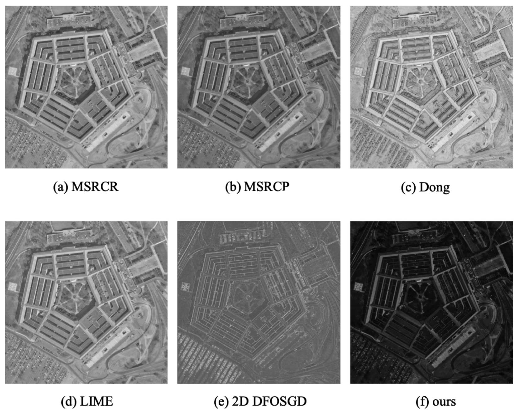
The comparison shows that the results of the proposed algorithm are better than the other algorithms except for the image “3.2.25”. To have a better understanding, we made a comparison between the results of two algorithms, as shown in
Figure 16.
From
Figure 16, it is observed that SSIM values of the other algorithms are higher, which is because their enhancement performances are not obvious. While the proposed algorithm preserves and enhances the image structure, it sensibly modifies the gray levels and leads to the lowest SSIM.
4.2.4. Measure of Enhancement by Entropy
The measure of enhancement by entropy (EMEE), proposed by Agaian et al. [
31], is based on the modification of Weber’s and Fisher’s Laws. EMEE uses Weber’s ratio in the calculation of entropy and gives the measure of contrast in terms of entropy [
32]. EMEE is more sensitive to change in contrast to other metrics, with a larger EMEE value indicating higher contrast in images. EMEE is defined as
where image
f is divided in to
blocks,
is a constant,
and
are the maximum and minimum values of the pixels in each block. The compared results are shown in
Table 4.
The comparison shows that the proposed algorithm has the second highest EMEE value among all the six algorithms. Moreover, while 2D DFOSGD has the highest EMEE value, it might lose information of an image as the high contrast will reduce the detail pattern.
4.2.5. Blind/Referenceless Image Spatial Quality Evaluator
The blind/referenceless image spatial quality evaluator (BRISQUE) [
33] is a model based on natural scene statistics and can measure image naturalness based on measured deviations from a natural image model. The first step of BRISQUE is extracting natural scene statistics and transforming image gray level to luminance. Then, we calculate fracture vectors and use a learning algorithm to evaluate the image quality score, with a smaller BRISQUE score indicating better perceptual quality. The comparison results are shown in
Table 5.
The results show that the proposed algorithm has the lowest BRISQUE for most of the test images, while for image “3.2.25” MSRCP and LIME have better performance. From
Figure 16, it is observed that the change in both algorithms is slight, which leads to the lower BRISQUE value.
5. Conclusions
In this paper, a new image enhancement algorithm based on a rough set and fractional order differentiator is proposed. In the proposed segmentation process, the rough set theory and Gaussian mixture model are combined to cluster gray levels into several image layers. In addition, compressing gray levels and filling in blank regions are performed to further centralize the information. Moreover, in the image enhancement process, 2D Fourier transform is employed to turn gray levels into a gradient, then an adaptive fractional order differential operator based on entropy is proposed to enhance the information of images. Experiments have verified the effectiveness of this algorithm. In the future, we intend to extend this enhancement process by studying more efficient segmentation methods and enhancement algorithms that can achieve higher structure similarities.
Author Contributions
Conceptualization, methodology, software, validation, X.Z. and L.D.; formal analysis, X.Z. and L.D.; investigation, X.Z. and L.D.; resources, X.Z. and L.D.; data curation, X.Z. and L.D.; writing—original draft preparation, L.D.; writing—review and editing, X.Z.; visualization, L.D.; supervision, X.Z.; project administration, X.Z.; funding acquisition, X.Z. All authors have read and agreed to the published version of the manuscript.
Funding
This research was funded by National Key Research and Development Program topic 2020YFB1710003.
Institutional Review Board Statement
Not applicable.
Informed Consent Statement
Not applicable.
Data Availability Statement
Not applicable.
Conflicts of Interest
The authors declare no conflict of interest.
References
- Chu, W.; Lee, K.T.; Luo, W.; Bhambri, P.; Kautish, S. Predicting the security threats of internet rumors and spread of false information based on sociological principle. Comput. Stand. Interfaces 2021, 73, 103454. [Google Scholar] [CrossRef]
- Khan, R.; Yang, Y.; Liu, Q.; Qaisar, Z.H. Divide and conquer: Ill-light image enhancement via hybrid deep network. Expert Syst. Appl. 2021, 182, 115034. [Google Scholar] [CrossRef]
- Deng, T.Q.; Sheng, C.D. Image threshold segmentation based on entropy of variable precision rough sets and genetic algorithm. Control Decis. 2011, 26, 1079–1082. [Google Scholar]
- Pal, S.; Mitra, P. Multispectral image segmentation using the rough-set-initialized EM algorithm. IEEE Trans. Geosci. Remote Sens. 2002, 40, 2495–2501. [Google Scholar] [CrossRef]
- Majak, M. Universal Segmentation Framework for Medical Imaging Using Rough Sets Theory and Fuzzy Logic Clustering. Adv. Intell. Syst. Comput. 2014, 283, 175–186. [Google Scholar] [CrossRef]
- Acharya, U.K.; Kumar, S. Genetic algorithm based adaptive histogram equalization (GAAHE) technique for medical image enhancement. Optik 2021, 230, 166273. [Google Scholar] [CrossRef]
- Krishna, R.; Kumar, S.S. Hybridizing differential evolution with a genetic algorithm for color image segmentation. Eng. Technol. Appl. Sci. Res. 2016, 6, 1182–1186. [Google Scholar] [CrossRef]
- Singh, V.; Misra, A.; Singh, V. Cardiac Image Segmentation using Improved Genetic Algorithm. Indian J. Sci. Technol. 2017, 10, 1–4. [Google Scholar] [CrossRef][Green Version]
- Chen, G.; Chen, Z. Regional classification of urban land use based on fuzzy rough set in remote sensing images. J. Intell. Fuzzy Syst. 2020, 38, 1–10. [Google Scholar] [CrossRef]
- Zhang, M.; Jiao, L.; Ma, W.; Ma, J.; Gong, M. Multi-objective Evolutionary Fuzzy Clustering for Image Segmentation with MOEA/D. Appl. Soft Comput. 2016, 48, 621–637. [Google Scholar] [CrossRef]
- Zhu, X.; Xiao, X.; Tjahjadi, T.; Wu, Z.; Tang, J. Image enhancement using fuzzy intensity measure and adaptive clipping histogram equalization. arXiv 2021, arXiv:2101.05922. [Google Scholar]
- Xiao, B.; Tang, H.; Jiang, Y.; Li, W.; Wang, G. Brightness and contrast controllable image enhancement based on histogram specification. Neurocomputing 2018, 275, 2798–2809. [Google Scholar] [CrossRef]
- Huang, Z.; Fang, H.; Li, Q.; Li, Z.; Zhang, T.; Sang, N.; Li, Y. Optical remote sensing image enhancement with weak structure preservation via spatially adaptive gamma correction. Infrared Phys. Technol. 2018, 94, 38–47. [Google Scholar] [CrossRef]
- Huang, D.; Wang, Y.; Song, W.; Sequeira, J.; Mavromatis, S. Shallow-water image enhancement using relative global histogram stretching based on adaptive parameter acquisition. In International Conference on Multimedia Modeling; Springer: Cham, Switzerland, 2018; pp. 453–465. [Google Scholar]
- Liu, K.; Tian, Y. Research and analysis of deep learning image enhancement algorithm based on fractional differential. Chaos Solitons Fractals 2020, 131, 109507. [Google Scholar] [CrossRef]
- Kaur, K.; Jindal, N.; Singh, K. Fractional Fourier Transform based Riesz fractional derivative approach for edge detection and its application in image enhancement. Signal Process. 2021, 180, 107852. [Google Scholar] [CrossRef]
- Singh, H.; Kumar, A.; Balyan, L.; Singh, G. A novel optimally weighted framework of piecewise gamma corrected fractional order masking for satellite image enhancement. Comput. Electr. Eng. 2019, 75, 245–261. [Google Scholar] [CrossRef]
- Pawlak, Z. Rough sets. Int. J. Comput. Inf. Sci. 1982, 11, 341–356. [Google Scholar] [CrossRef]
- Nguyen, T.M.; Wu, Q.J. Dirichlet Gaussian mixture model: Application to image segmentation. Image Vis. Comput. 2011, 29, 818–828. [Google Scholar] [CrossRef]
- Zhang, J.X.; Yang, G.H. Low-complexity tracking control of strict-feedback systems with unknown control directions. IEEE Trans. Autom. Control 2019, 64, 5175–5182. [Google Scholar] [CrossRef]
- Zhang, J.X.; Yang, G.H. Robust adaptive fault-tolerant control for a class of unknown nonlinear systems. IEEE Trans. Ind. Electron. 2016, 64, 585–594. [Google Scholar] [CrossRef]
- Yang, Q.; Chen, D.; Zhao, T.; Chen, Y. Fractional Calculus In Image Processing: A Review. Fract. Calc. Appl. Anal. 2016, 19, 1222–1249. [Google Scholar] [CrossRef]
- Zhang, X.; Chen, Y. Admissibility and robust stabilization of continuous linear singular fractional order systems with the fractional order α: The 0 < α < 1 case. ISA Trans. 2018, 82, 42–50. [Google Scholar] [PubMed]
- Mohabey, A.; Ray, A. Rough set theory based segmentation of color images. In Proceedings of the PeachFuzz 2000—19th International Conference of the North American-Fuzzy Information Processing Society-NAFIPS (Cat. No. 00TH8500), Atlanta, GA, USA, 13–15 July 2000; pp. 338–342. [Google Scholar]
- Shannon, C.E. Communication theory of secrecy systems. MD Comput. 1998, 15, 57–64. [Google Scholar] [CrossRef] [PubMed]
- Chen, D.; Chen, Y.; Xue, D. 1-D and 2-D digital fractional-order Savitzky-Golay differentiator. Signal Image Video Process. 2012, 6, 503–511. [Google Scholar] [CrossRef]
- Guo, X.; Li, Y.; Ling, H. LIME: Low-light image enhancement via illumination map estimation. IEEE Trans. Image Process. 2016, 26, 982–993. [Google Scholar] [CrossRef]
- Dong, X.; Wang, G.; Pang, Y.; Li, W.; Wen, J.; Meng, W.; Lu, Y. Fast efficient algorithm for enhancement of low lighting video. In Proceedings of the 2011 IEEE International Conference on Multimedia and Expo, Barcelona, Spain, 11–15 July 2011; pp. 1–6. [Google Scholar]
- Petro, A.B.; Sbert, C.; Morel, J.M. Multiscale Retinex. Image Process. Line 2014, 4, 71–88. [Google Scholar] [CrossRef]
- Zhou, W.; Bovik, A.C.; Sheikh, H.R.; Simoncelli, E.P. Image quality assessment: From error visibility to structural similarity. IEEE Trans. Image Process. 2004, 13, 600–612. [Google Scholar] [CrossRef]
- Agaian, S.S.; Panetta, K.; Grigoryan, A.M. Transform-based image enhancement algorithms with performance measure. IEEE Trans. Image Process. 2001, 10, 367–382. [Google Scholar] [CrossRef]
- Prajapati, P.; Narmawala, Z.; Darji, N.P.; Moorthi, S.M.; Ramakrishnan, R. Evaluation of perceptual contrast and sharpness measures for meteorological satellite images. Procedia Comput. Sci. 2015, 57, 17–24. [Google Scholar] [CrossRef]
- Mittal, A.; Moorthy, A.K.; Bovik, A.C. Blind/Referenceless Image Spatial Quality Evaluator. In Proceedings of the 2011 Conference Record of the Forty Fifth Asilomar Conference on Signals, Systems and Computers (ASILOMAR), Pacific Grove, CA, USA, 6–9 November 2011; pp. 723–727. [Google Scholar] [CrossRef]
Figure 1.
The relationship between R-upper and R-lower approximations of set X.
Figure 1.
The relationship between R-upper and R-lower approximations of set X.
Figure 2.
A Gaussian mixture model.
Figure 2.
A Gaussian mixture model.
Figure 3.
Fourier transform frequency image of image “3.2.25”.
Figure 3.
Fourier transform frequency image of image “3.2.25”.
Figure 4.
Fractional differential of different for different orders .
Figure 4.
Fractional differential of different for different orders .
Figure 5.
A four-direction fractional order differentiator mask.
Figure 5.
A four-direction fractional order differentiator mask.
Figure 6.
The segmentation results of image “3.2.25”.
Figure 6.
The segmentation results of image “3.2.25”.
Figure 7.
The comparison of preprocessed results of image “3.2.25”.
Figure 7.
The comparison of preprocessed results of image “3.2.25”.
Figure 8.
The Fourier frequency images of the filtered image by and and their inverse transform results.
Figure 8.
The Fourier frequency images of the filtered image by and and their inverse transform results.
Figure 9.
The process of the proposed algorithm where denotes the optimal image.
Figure 9.
The process of the proposed algorithm where denotes the optimal image.
Figure 10.
Enhancement results of image “2.1.01”.
Figure 10.
Enhancement results of image “2.1.01”.
Figure 11.
Enhancement results of image “2.1.02”.
Figure 11.
Enhancement results of image “2.1.02”.
Figure 12.
Enhancement results of image “2.1.03”.
Figure 12.
Enhancement results of image “2.1.03”.
Figure 13.
Enhancement results of image “2.2.01”.
Figure 13.
Enhancement results of image “2.2.01”.
Figure 14.
Enhancement results of image “2.2.02”.
Figure 14.
Enhancement results of image “2.2.02”.
Figure 15.
Enhancement results of image “3.2.25”.
Figure 15.
Enhancement results of image “3.2.25”.
Figure 16.
The comparison of the enhancement results.
Figure 16.
The comparison of the enhancement results.
Table 1.
The comparison of information entropy.
Table 1.
The comparison of information entropy.
| File Name | Original Image | MSRCR
[29] | MSRCP
[29] | Dong
[28] | LIME
[27] | 2D
DFOSGD [26] | Ours |
|---|
| 2.1.01 | 7.1953 | 6.0504 | 6.8504 | 7.2276 | 7.1749 | 7.4801 | 7.0126 |
| 2.1.02 | 7.1957 | 5.6973 | 7.3305 | 7.2253 | 6.9049 | 7.5231 | 7.4305 |
| 2.1.03 | 5.7432 | 5.0140 | 5.9454 | 6.2486 | 6.0599 | 6.1488 | 6.1326 |
| 2.2.01 | 7.5383 | 6.5375 | 7.3525 | 7.4967 | 7.4986 | 7.4258 | 7.4216 |
| 2.2.02 | 5.5966 | 5.5984 | 5.6934 | 5.8297 | 5.6365 | 4.9948 | 6.4338 |
| 3.2.25 | 6.7327 | 6.8914 | 6.7327 | 6.9222 | 6.0745 | 6.3865 | 6.6088 |
Table 2.
The comparison of PSNR.
Table 2.
The comparison of PSNR.
| File Name | MSRCR | MSRCP | Dong | LIME | 2D DFOSGD | Ours |
|---|
| 2.1.01 | 14.9695 | 12.9041 | 16.8970 | 12.7384 | 16.9118 | 16.3130 |
| 2.1.02 | 16.6889 | 23.8252 | 21.2345 | 15.0227 | 17.6716 | 29.8310 |
| 2.1.03 | 16.4032 | 22.0502 | 16.6842 | 16.8729 | 24.4056 | 26.0449 |
| 2.2.01 | 14.2120 | 12.9945 | 18.3624 | 14.1881 | 16.1057 | 19.5256 |
| 2.2.02 | 21.6140 | 18.9519 | 20.8912 | 18.3157 | 19.4603 | 13.8081 |
| 3.2.25 | 19.3656 | 32.9054 | 14.5181 | 9.7675 | 19.3744 | 24.0654 |
Table 3.
The comparison of SSIM.
Table 3.
The comparison of SSIM.
| File Name | MSRCR | MSRCP | Dong | LIME | 2D DFOSGD | Ours |
|---|
| 2.1.01 | 0.7365 | 0.3635 | 0.8799 | 0.8896 | 0.6338 | 0.9191 |
| 2.1.02 | 0.7067 | 0.9723 | 0.9522 | 0.9510 | 0.7048 | 0.9840 |
| 2.1.03 | 0.8725 | 0.9508 | 0.8917 | 0.9612 | 0.7859 | 0.9589 |
| 2.2.01 | 0.6972 | 0.4814 | 0.9080 | 0.9128 | 0.5939 | 0.9148 |
| 2.2.02 | 0.8600 | 0.9196 | 0.9563 | 0.9817 | 0.8701 | 0.8472 |
| 3.2.25 | 0.9330 | 0.9978 | 0.8071 | 0.8379 | 0.6909 | 0.4758 |
Table 4.
The comparison of EMEE ().
Table 4.
The comparison of EMEE ().
| File Name | MSRCR | MSRCP | Dong | LIME | 2D DFOSGD | Ours |
|---|
| 2.1.01 | 0.5703 | 1.2858 | 1.3631 | 1.2298 | 1.6667 | 1.6917 |
| 2.1.02 | 0.5641 | 1.1045 | 1.2107 | 1.1868 | 2.6192 | 1.2085 |
| 2.1.03 | 1.6893 | 1.4232 | 1.4570 | 1.4578 | 6.8302 | 2.1350 |
| 2.2.01 | 1.6194 | 1.2754 | 1.4351 | 1.2190 | 1.4122 | 1.3887 |
| 2.2.02 | 0.9698 | 0.5425 | 0.8565 | 0.7802 | 1.3538 | 1.2693 |
| 3.2.25 | 0.6713 | 0.6699 | 0.9298 | 0.7660 | 1.2178 | 1.8949 |
Table 5.
The comparison of BRISQUE.
Table 5.
The comparison of BRISQUE.
| File Name | MSRCR | MSRCP | Dong | LIME | 2D DFOSGD | Ours |
|---|
| 2.1.01 | 36.3670 | 45.0807 | 43.3830 | 36.4630 | 45.3041 | 30.0843 |
| 2.1.02 | 27.1624 | 42.9080 | 43.4556 | 43.4614 | 44.5253 | 41.2102 |
| 2.1.03 | 42.4831 | 23.2094 | 26.3333 | 21.1117 | 39.8493 | 17.4546 |
| 2.2.01 | 42.8555 | 41.9647 | 37.3137 | 33.1370 | 33.0672 | 30.7001 |
| 2.2.02 | 43.3932 | 33.3401 | 30.3013 | 26.3762 | 38.2801 | 26.9195 |
| 3.2.25 | 35.2187 | 22.8275 | 43.3979 | 28.9676 | 43.1892 | 32.5178 |
| Publisher’s Note: MDPI stays neutral with regard to jurisdictional claims in published maps and institutional affiliations. |
© 2022 by the authors. Licensee MDPI, Basel, Switzerland. This article is an open access article distributed under the terms and conditions of the Creative Commons Attribution (CC BY) license (https://creativecommons.org/licenses/by/4.0/).
