Continuum Damage Dynamic Model Combined with Transient Elastic Equation and Heat Conduction Equation to Solve RPV Stress

Abstract

The development of the world cannot be separated from energy: the energy crisis has become a major challenge in this era, and nuclear energy has been applied to many fields. This paper mainly studies the stress change of reaction pressure vessels (RPV). We established several different physical models to solve the same mechanical problem. Numerical methods range from 1D to 3D; the 1D model is mainly based on the mechanical equilibrium equations established by the internal pressure of RPV, the hoop stress, and the axial stress. We found that the hoop stress is twice the axial stress; this model is a rough estimate. For 2D RPV mechanical simulation, we proposed a new method, which combined the continuum damage dynamic model with the transient cross-section finite element method (CDDM-TCFEM). The advantage is that the temperature and shear strain can be linked by the damage factor effect on the elastic model and Poission ratio. The results show that with the increase of temperature (damage factor $\widehat{\mu },\widehat{d}$), the Young’s modulus decreases point by point, and the Poisson’s ratio increases with the increase of temperature (damage factor $\widehat{\mu },{\mathcal{E}}_{\mathrm{t}}$). The advantage of the CDDM-TCFEM is that the calculation efficiency is high. However, it is unable to obtain the overall mechanical cloud map. In order to solve this problem, we established the axisymmetric finite element model, and the results show that the stress value at both ends of RPV is significantly greater than that in the middle of the container. Meanwhile, the shape changes of 2D and 3D RPV are calculated and visualized. Finally, a 3D thermal–mechanical coupling model is established, and the cloud map of strain and displacement are also visualized. We found that the stress of the vessel wall near the nozzle decreases gradually from the inside surface to the outside, and the hoop stress is slightly larger than the axial stress. The main contribution of this paper is to establish a CDDM-TCFEM model considering the influence of temperature on elastic modulus and Poission ratio. It can dynamically describe the stress change of RPV; we have given the fitting formula of the internal temperature and pressure of RPV changing with time. We also establish a 3D coupling model and use the adaptive mesh to discretize the pipe. The numerical discrete theory of FDM-FEM is given, and the numerical results are visualized well. In addition, we have given error estimation for h-type and p-type adaptive meshes. So, our research can provide mechanical theoretical support for nuclear energy safety applications and RPV design.

1. Introduction

1.1. Research Motivation and Significance

Nuclear energy plays an important role in today’s energy system, especially nuclear power generation. Nuclear energy is a safe, clean, and economical energy source [1]. Meanwhile, it has many advantages, such as the small size of reaction equipment, slowing down the greenhouse effect, and releasing huge energy in a short time. The main negative impact is that nuclear accidents are prone to nuclear radiation and nuclear pollution. Therefore, the quality of nuclear pressure vessels must be up to standard before they can be used, including operating specifications, regular security inspections, etc. The design of pressure vessels and safety performance evaluation is also an important research topic [2,3]. The force analysis of RPV will also use some knowledge of extreme mechanics, especially for the welding joints of nuclear reactor nozzles. Due to the limited load, stress concentration and various cracks are prone to occur here. The ultimate load is mainly determined by the overall plastic yield of the shell material [4,5]. When the yield strength is low, it has almost no effect on the crack size. As yields increase, cracks will also increase. Since the pressure vessel is operated in a high-temperature environment, many physical parameters will change, such as the density, Young modulus, Poisson ratio, and so on. In fact, during normal operation, nuclear pressure vessels are in a multi-physics environment, such as operating under the combined effects of high temperature, thermal shock, coolant, nuclear radiation, etc. In addition, temperature and thermal shock may cause corrosion and damage to the RPV cladding. These factors are essential in the design of RPV and in the later stage of quality inspection. However, there are few theories and models in this field that need to be improved urgently, which is the purpose and significance of our research.

1.2. Related Work

In addition, pressure vessel is the core component of the design and operation of next-generation reactors. Fatigue damage analysis, crack propagation simulation, and pipe opening stress calculation are usually required for RPV. However, many models belong to static mechanical analysis, and the Young’s modulus and Poisson’s ratio of the model are calculated according to fixed values. A damage model was established to describe the dynamic changes of Young’s modulus and Poisson’s ratio. The reliability of RPV also includes some uncertain factors, including the existence of the coupling of internal pressure and inertial force, combined with probabilistic fracture mechanics, estimation of stress intensity factors, and in turn, these works can help to analyze the pressure vessel’s fracture and reliability analysis [6,7]. The mechanical properties and electromagnetic properties are the external performance under irradiation [8]. These advantages are beneficial to establish the nondestructive evaluation technology of embrittlement. Numerical calculation combined with the local nonlinear dynamics method and this criterion based on the critical splitting stress have greatly improved the global static method to describe the crack propagation.

The structural damage dynamic model is usually used in combination with the fatigue analysis model. In continuum mechanics, the damage is calculated as a post-processing of elastic or elastoplastic macroscopic analysis. However, this important work has not been cited in the mechanical research of RPV, which also reflects the uniqueness of our work. The damage is considered to be isotropic, and there is a micro-defect closure effect on both macro and micro scales [9]. Secondly, the damage evolution equation can explain different damage mechanisms when forging alloy materials. The numerical results show that the damage evolution equation can reflect the anisotropic accelerated creep and creep fracture time under different stress levels and loading directions [10]. Through the numerical simulation of the representative volume element (RVE) of quasi-brittle materials, an anisotropic damage model with the least internal variables can be constructed [11]. The orientation distribution function of the two elastic modulus is numerically determined, and the influence of the nucleation and propagation of microcracks is considered by the phase field method. In reference [12], an energy-based damage model is proposed to simulate the crack propagation of very low cycle fatigue (VLCF). This model can be used to predict the failure period, and the comparison of fracture surfaces also shows good consistency. The above model is only applicable to the damage model of a mechanical single field independent of temperature change, which also reflects that the research work in this paper is different from the current model. We consider the influence of physical information such as temperature and shear strain on the material. The fatigue damage analysis of RPV requires a variety of theories to solve, including prediction of the crack growth of steel RPV based on the maximum main stress propagation standard and combination with the probability direction standard to predict the unstable crack path [13,14,15].

The cross-section FEM has the characteristics of fast calculation, stratification, and local mechanics, and it has been widely used to solve various engineering problems [16,17,18]. However, they are all numerical theories of the static cross-section FEM, and there are few transient cross-section FEM methods. Transient energy studies the mechanical changes in each time period, which is wider than the static practical range. This is also the reason why this paper uses the transient cross-section FEM to study the nuclear pressure vessel. Changsik provides a simple method to estimate the cross-section stress distribution of the nozzle designed according to Section 3 of the ASME code. This method requires the geometric information of pressure vessels and nozzles. The limitation of this method is that the stress distribution in the cross-section needs to use accurate stress concentration factors, and the method discussed is only effective under internal pressure [19]. The error of the RPV stress theoretical analysis method for 2D cross-section FEM analysis is relatively large at the edge. Reference [20] derived the accurate theoretical formulas of radial and axial displacement of cylindrical vessels and pipelines under thermal stress through the fourth-order differential equation. The edge effect has an important influence on the geometric deformation of pressure vessels and pipelines under thermal mechanical load. The maximum relative error of radial displacement at the edge reaches 42.2%, and the maximum relative error of axial displacement reaches 28.5%. Sectional FEM is also used to study the influence of buckling and post-buckling behavior of composite laminates [21]. The results are compared with those of two finite element models. Residual stresses have a significant influence on the buckling and post-buckling behavior of closed-section thin-walled laminated structures.

Recently, there have been some simulation models of RPV. The study of stress intensity of the RPV pipe mouth is generally controlled by parameters such as size, shape, inner radius and thickness of the nozzle, etc. It is concluded that the optimal design of the nozzle can minimize the stress intensity (Tresca yield criterion) and conflict between the quality of RPV [22]. However, the working environment of RPV belongs to multi-physics and needs to consider the interaction of temperature and stress, which is also the difference of the nozzle model established in our paper. In addition, we also compare the axial stress and hoop stress. What is more, through simulation, three-dimensional thermal hydraulic parameter distributions can be obtained; with the increase of the injection rate, the disturbance of the temperature field and the velocity field becomes more intense, and it is more likely to cause thermal fatigue [23,24].

Pressurized thermal shock (PTS) also affects the structural integrity of the pressurized water RPV. The literature [25,26] studies the pressurization–thermal shock phenomenon in pressure vessels (RPV). The results show that the assessment of crack initiation, stopping, and tearing instability in thermal shock (PTS) events (of RPV) is studied. According to the new results, the tearing process of RPV is still stable even for large initial cracks larger than the maximum assumed crack size in the code [27,28]. The most important performance factor is mainly the application of fluid and probabilistic fracture mechanics to comprehensively evaluate the structural integrity of RPV under hypothetical PTS accidents. When the emergency nuclear cooling (ECC) water is injected, a large temperature gradient will be generated, which will lead to a large thermal stress in the RPV wall. Predicting the thermo-mechanical behavior of the pressure vessel can also improve the safe coefficient, optimizing the ECCS performance [29,30]. Other literature work thermal shock force is generally in the form of a graph. In this paper, the fitting formula of thermal shock force and temperature is given, which is convenient for outputting the function value corresponding to any moment during the simulation process.

In addition, regarding the issue of stress prediction, synchronization accelerator X-ray diffraction measures the stress generated by the clad pressure vessel steel during thermal shock. Experimental measurements show that the peak stress intensity factor occurs during thermal shock, rather than in a steady state [31]. The internal structure of the pressure vessel is more complicated and accompanied by robust radiation, so the experimental measurement is relatively difficult. At present, ultrasonic technology can be used to measure the stress of the pressure vessel, and ultrasonic transducers with different frequency ranges are used to evaluate the hoop and axial residual stress [32]. The experiment indicates that it is limited, the calculated stress and ultrasonic measurement results have a high degree of consistency. In addition, the elements added in RPV steel will affect the toughness and crack resistance of the material. Figure 1 below shows the evolution of the main chemical elements of RPV in China in the last 40 years. The key properties of nuclear RPV are high strength, good toughness, corrosion resistance, good compatibility with coolant, stable microstructure, good welding, hot and cold processing performance, and developing to an ultra-high strength direction.

Furthermore, there are also many numerical methods for pressure vessel stress evaluation, such as the extended 3D finite element method (XFEM) to calculate the stress field of the reactor pressure vessel (RPV). The sub-model contains three types of cracks: axial, circumferential, and inclined directions [33]. However, there are a few coupling field simulation models with time term for RPV. In this paper, the transient thermal–mechanical coupling model is studied, which is different from other research work. We use FDM-FEM to discrete the 3D pipeline port area. In addition, there are also multi-scale coupled numerical methods for force analysis of pressure vessels [34], and simulation of thermo-hydraulic phenomena (such as heat, mass, and dissolution transmission in nuclear pressure vessels (RPV)). Four subsystems have been solved; the parameter correlation of RPV can more realistically react the heat transfer simulation of the pressure vessel. Reference [35] FVM is reliable for solving the neutron diffusion equation, and it can obtain an accurate three-dimensional distribution of neutron flux and power of the core. For a metal pressure vessel, generally, corrosion-resistant materials are used to prevent the material from becoming fragile due to rust and chemical attack, and the tensile strength will be reduced. Eventually, it will cause bursting under high internal pressure. Actual nuclear pressure vessels are composite materials. There are many finite element methods for pressure vessel structures/components and pipelines [36]. They even include linear and nonlinear, static and dynamic, stress and deflection analysis, thermal problems, fracture mechanics problems, and solid coupling [37,38]. COMSOL, ANSYS, ABAQUES, etc. are commonly used in the finite element analysis software of pressure vessels and pipelines.

1.3. Contributions

The main contributions of this article are four points. Firstly, this paper proposed a simplified one-dimensional RPV estimation formulas for axial and hoop stress and introduces the working principle of RPV. The second contribution is that we proposed the continuous damage dynamics model combined with the transient cross-section FEM Method (CDDM-TCFEM), which can adapt to the variable parameter mechanical calculation model in the high-temperature environment. The change trend of Young’s modulus and Poisson ratio is calculated and visualized. The third contribution is that we use axisymmetric FEM to analyze the nuclear pressure vessel, which not only improves the calculation speed but also obtains the overall mechanical change cloud map. A variable parameter model is more accurate than traditional fixed parameter calculation. In addition, we found that the stress at both ends of the RPV was significantly greater than that in the middle. The fourth contribution is that we build the physical model of the mechanical and thermal coupling, analyze the mechanical change of the RPV pipe mouth, and calculate the difference between the pipe mouth axial stress and loop stress, and finally the specific temperature and mechanical change cloud diagrams are given. In a word, our work is beneficial to the structural design and the RPV’s security assessment.

1.4. Structure and Framework of This Paper

The structural arrangement and design of this paper consists of five sections. Section 2 mainly consists of two parts. Part one is a one-dimensional simplified mechanical equilibrium problem, which describes the internal pressure and axial stress, and the equilibrium problem of hoop stress. Part two mainly introduces the continuous damage dynamic model and the numerical theory of cross-section finite element (DDM-TSFEM). We convert it into a two-dimensional section to solve. Section 3 mainly introduces the axisymmetric finite element method. We obtained the three-dimensional stress–strain cloud map of the pressure vessel through thermal shock force, which is more intuitive than the section finite element method. Another feature of this model is the addition of deformation. Section 4 is mainly about the thermal field–force field coupling of the RPV pipe mouth physical model. By establishing three-dimensional transient solid heat transfer and elastic mechanics equations, the axial and radial stress variation trends are finally obtained at different times. The biggest feature of this example is that the stress change at the RPV nozzle is considered. Section 5 is mainly a summary and outlook and provides the relevant research conclusions of this paper and the problems that need to be studied subsequently.

2. RPV Working Principle and Internal Structure of Nuclear Power

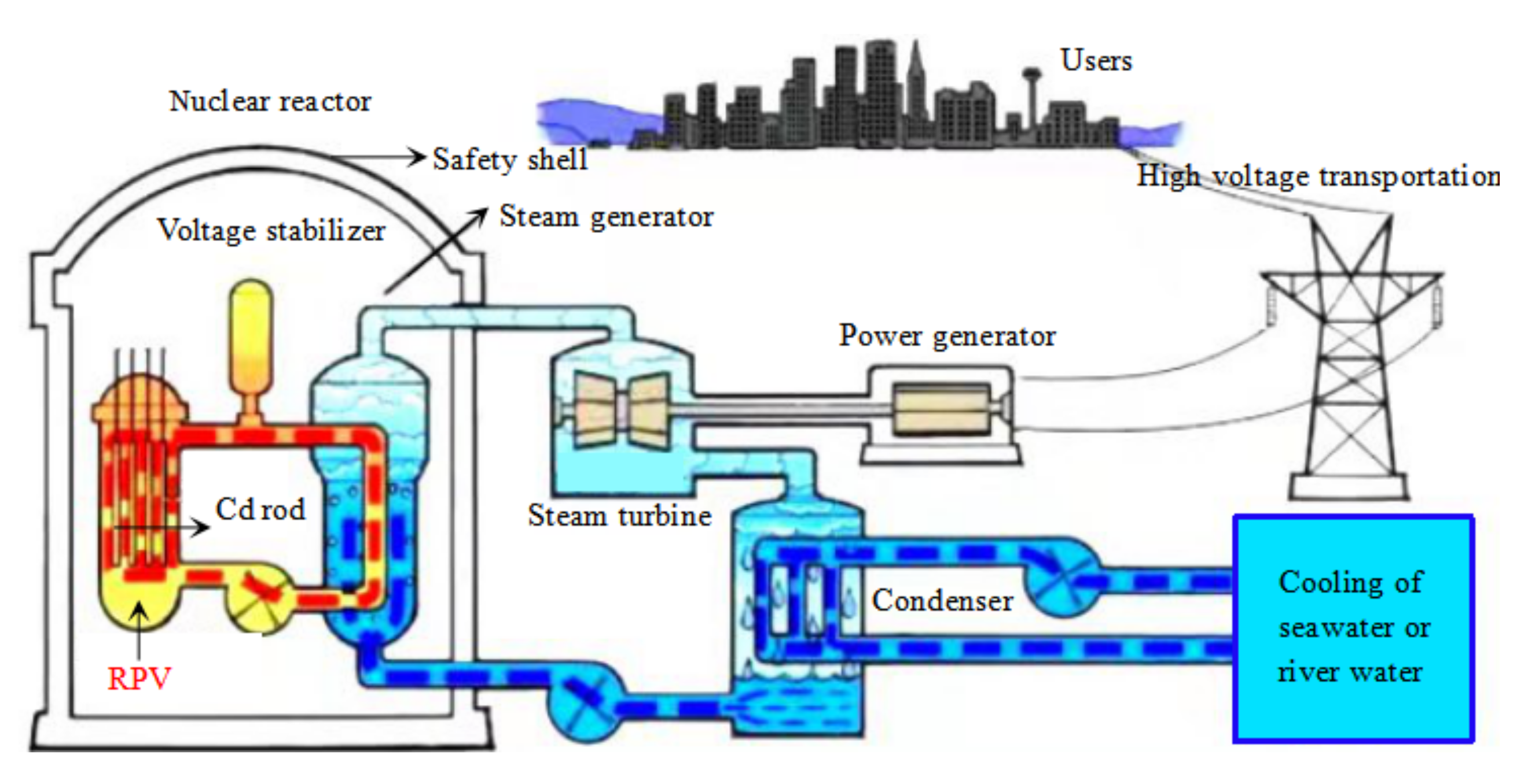
2.1. RPV Working Principle of Nuclear Power

Nuclear power plants can convert nuclear energy into electrical energy for life and industrial use. The core component of nuclear power plants is nuclear pressure vessels. Common nuclear power plants can be divided into pressurized water reactor nuclear power plants, heavy water reactor nuclear power plants, boiling water reactor nuclear power plants, and fast reactor nuclear power plants according to different reactor principles. At present, China’s main nuclear power plants are composed of pressurized water reactor nuclear power plants and heavy water reactor nuclear power plants. More than 60% of the world ’s nuclear power plants are PWR nuclear power plants, which are mainly composed of reactors, steam generators, steam turbines, generators, and related system equipment.

At present, in nuclear power plants, the role of reactors is to conduct nuclear fission and convert nuclear energy into heat energy from water. Water as a coolant absorbs the heat generated by nuclear fission in the reactor, and water at high temperature and high pressure becomes saturated steam. The steam pressure promotes the rotation of the steam turbine, and the heat energy is converted into mechanical energy. Then, the steam turbine drives the generator to rotate and converts mechanical energy into electrical energy. The cooled water is pumped back to the reactor by the main pump and heated again. Thus, the cycle is repeated to form a closed cycle of heat absorption and heat release. The pressure of the loop is controlled by the regulator. Usually, the primary circuit and its auxiliary systems and plants are collectively referred to as nuclear islands (NIs). In summary, the PWR nuclear power plant converts nuclear energy into electrical energy in four steps, which are implemented by four main devices:

(a)

Reactor—converting nuclear energy into water heat.

(b)

Steam generator—transferring the heat from the high-temperature and high-pressure water in the first loop to the water in the second loop, so that it becomes saturated steam.

(c)

Steam turbine—converting the heat energy of saturated steam into the mechanical energy of high-speed rotation of a steam turbine rotor.

(d)

Generator—converting mechanical energy from the steam turbine into electrical energy. To use power generation, they need to go through multiple complex processes. The working principle diagram of the pressurized water reactor nuclear power plant is shown in Figure 2.

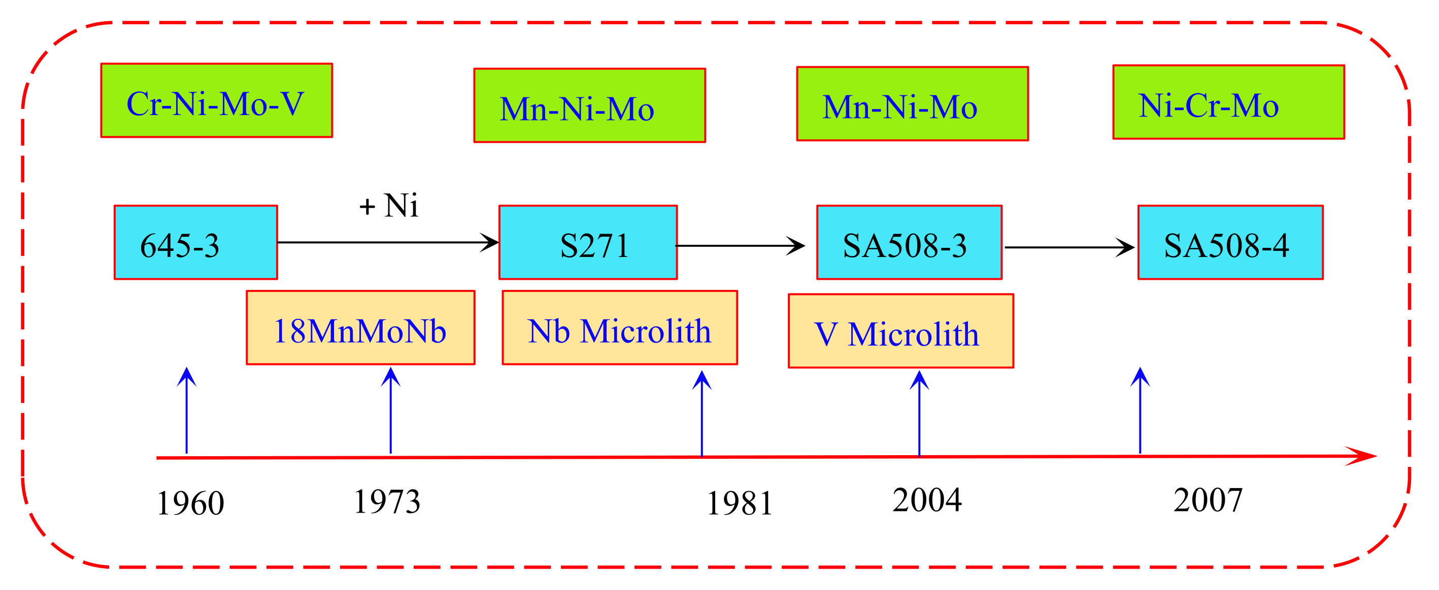
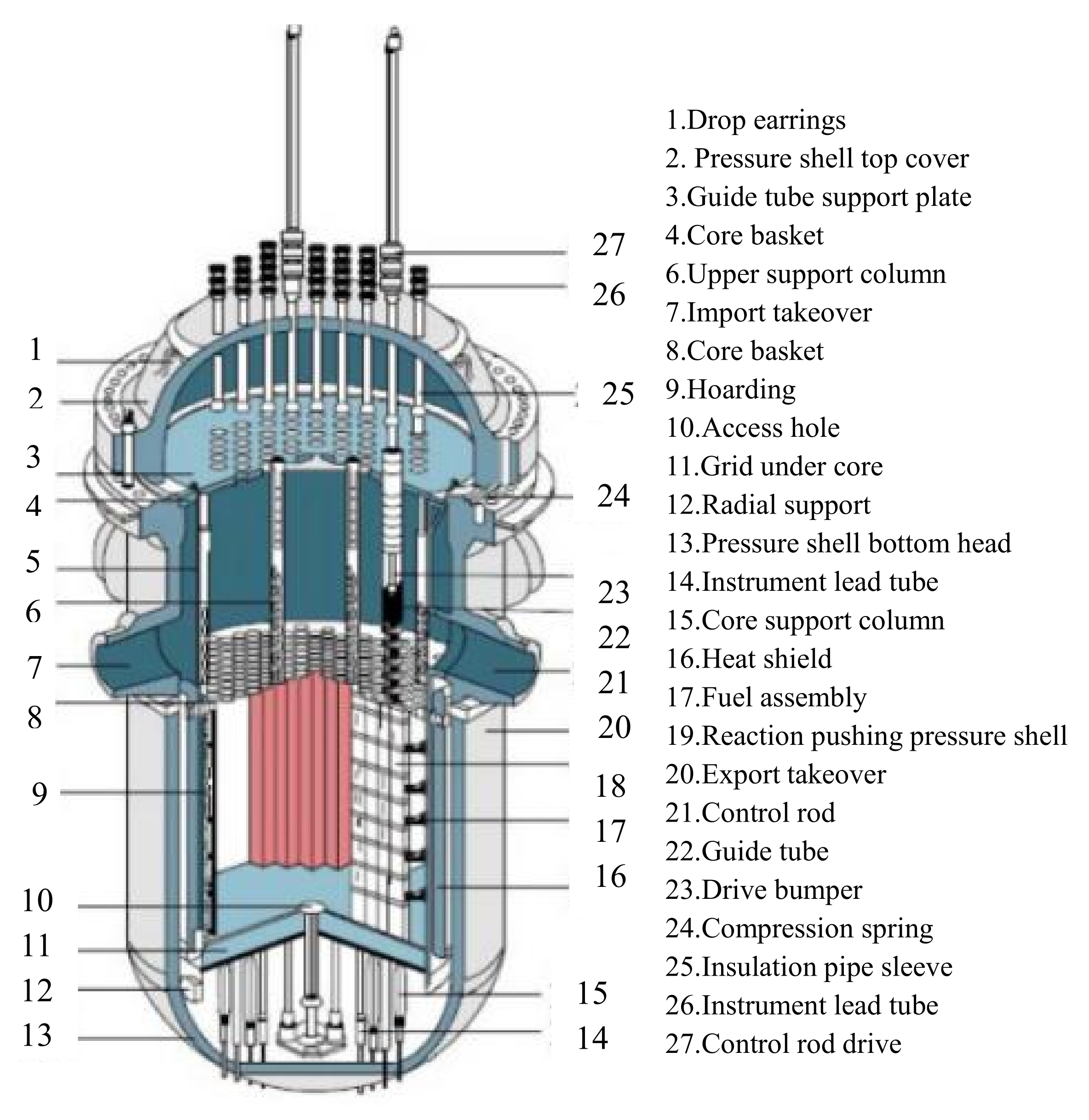
2.2. RPV Classification and Internal Structure

The nuclear pressure vessel is an important device of nuclear power plants. High-strength alloy steel (Fe, Mn, C, Zn, and other elements) is generally used in the vessel. The internal material of the nuclear pressure vessel will encounter thermal impact force, high temperature, strong radiation, crack propagation, chemical corrosion, and other factors when working. It is difficult to measure the internal force by a direct experiment method. Therefore, the finite element method can be used to solve the numerical solution according to the elastic equation and boundary information. Example 1 mainly introduces the geometric two-dimensional transient elastic equation of the continuum damage dynamic model to solve the internal force of the nuclear pressure vessel. Common pressure vessels can be divided into four grades according to temperature and internal pressure. The classification results and scope standards are shown in

Table 1. Classification of nuclear pressure vessels by temperature and pressure.

Pressure Classification	Pressure Range	Temperature Classification	Temperature Range
Low-pressure vessel (L)	$0.1\mathrm{Mpa}\le P<1.6\mathrm{Mpa}$	Cryogenic container	$t<-20$${}^{°}$C
Medium-pressure vessel (M)	$1.6\mathrm{Mpa}\le P<10\mathrm{Mpa}$	Normal-temperature vessel	−20 ${}^{°}$C $\le t<$ 150 ${}^{°}$C
High-pressure vessel (H)	$10\mathrm{Mpa}\le P<100\mathrm{Mpa}$	Medium-temperature vessel	150 ${}^{°}$C $\le t<$ 450 ${}^{°}$C
Super-high-pressure vessels (U)	$P\ge 100\mathrm{Mpa}$	High-temperature vessels	$t\ge$ 450 ${}^{°}$C

.

The geometric dimensions of common nuclear reactor pressure vessels are generally ellipsoidal spherical vessels. The inner shell of the pressure vessel is made of harder steel materials such as austenitic stainless steel. Pressure vessels are commonly used key equipment in the nuclear power plant, petrochemical, metallurgical, power generation and aerospace sectors. They generally work in high temperature, high pressure, corrosion and radiation environments. Especially nuclear pressure vessels, strong neutron radiation will also cause continuous damage to the material and cause brittle fracture. In severe cases, there is a risk of explosion. Therefore, pressure vessel design and internal load control must be strictly implemented in accordance with the regulations. Currently, nuclear power plants mainly use nuclear fission to release energy. The internal structure of the nuclear pressure vessel is shown in Figure 3.

2.3. Four Model Assumptions of RPV

Before establishing the RPV model in this article, we need to give the assumptions of each model, which will help the model to describe the scope of use more accurately.

Model 1: This model assumes that the material is isotropic, the internal pressure is uniform, and the thickness of the container wall is greater than $d_m\ge$ 0.05 m.

Model 2: The CDDM-TCFEM method assumes that the obtained cross-sections are all continuous and uniform, isotropic materials. It satisfies the six assumptions of linear elasticity theory, including continuity, complete elasticity, uniformity, isotropy, slight deformation, and no initial stress. It is assumed that the continuous damage is a small defect, no obvious crack is formed, and the temperature will not cause the creep of the RPV vessel wall.

Model 3: The axisymmetric model assumes that the RPV shell is a symmetrical geometry, and the interior is subjected to a uniform outward pressure P.

Model 4: The thermal–mechanical coupling model of the pipe mouth assumes that the RPV material is isotropic; the process we study only emits hot steam and does not release the cooling liquid, because the release of the cooling liquid requires the addition of the hydrodynamic Navier–Stokes equation. We assume that at each moment, the temperature and pressure values remain relatively stable, and there is no sudden increase or decrease.

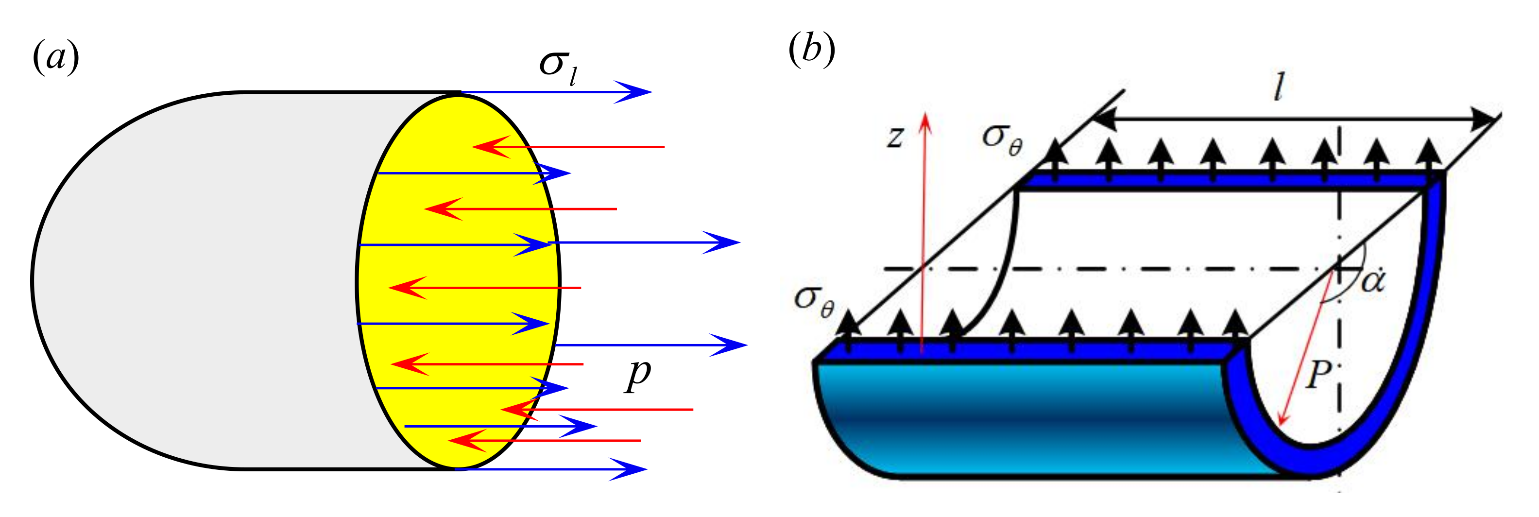
3. RPV Stress by the Simple Mechnical Balance

Model 1: Considering a simplified pressure vessel force analysis model, this vessel with radius r and wall thickness d is subjected to an internal gage pressure or thermal shock p along the longitudinal direction and hoop direction of the vessel to analyze the longitudinal stress ${\sigma }_l$ and hoop stress ${\sigma }_{\theta }$. This model has axisymmetric coordinates; there is no shear stress. When the working condition of the nuclear pressure vessel is stable, we make a cut across the section of the RPV to analyze the longitudinal stress ${\sigma }_l$ of the spherical pressure vessel.

Although the derivation process of the problem borrows the area to represent the axial stress ${\sigma }_l$ and the surface pressure F generated by the internal pressure P, the final formula shows that the radius R and the thickness $d_m$ of the vessel are constant, and the final change of the axial stress depends only on the internal pressure of the RPV. Therefore, the axial stress obtained by the model belongs to a simplified one-dimensional approximation.

$${\sigma }_l·d_m·2\pi r=p·\pi r^2,{\sigma }_l=\frac{pr}{2d_m}.$$

(1)

Similarly, the circumferential stress is also symmetrical. We cut the vessel along any axis. The tangential direction of the cylinder is the circumferential stress ${\sigma }_{\theta }$, and the equilibrium equation is established along the z direction. D is the diameter of the RPV, the pressure P acts on the projection of the half section, and $S=\frac{D}{2}lsin\alpha$ is balanced with the circumferential stress ${\sigma }_{\theta }$ acting on the two sections. We can finally get:

$${\int }_0^{\pi }pl\frac{D}{2}sin\alpha d\alpha =p·2r·d_m=2d_{m}l{\sigma }_{\theta },{\sigma }_{\theta }=\frac{pr}{d_m}.$$

(2)

The above model is only a one-dimensional static analysis on the cross section, and the calculated stress results are rough estimates. In fact, the three-dimensional force analysis of the nuclear RPV cannot be obtained by this method. We also want to get the local stress defects of the pressure vessel and the overall stress changes. When the nuclear vessel reacts, the inside is affected by thermal shock. The following sections will introduce the other two nuclear pressure vessel force analysis methods in detail. They are the cross-section method and the axisymmetric method. The hoop stress and axial stress in static equilibrium are illustrated in Figure 4.

4. Continuum Damage Dynamics Model with Transient Cross-Section FEM

4.1. Continuum Damage Dynamics Model

This section will introduce our proposed method continuum damage dynamics model with transient cross-section FEM in detail, which is referred to as the CDDM-TCFEM method. This model mainly assumes that the nuclear pressure vessel is an isotropic material. A large amount of heat will be released instantaneously during the nuclear fission reaction. The surrounding gas will form thermal shock, long-term erosion, high-temperature effects, and microscopic cracks formed on the inner surface of the pressure vessel. Residual stress cannot be ignored and will have a certain impact on the container itself. In order to accurately describe the magnitude of the impact, we established a continuum dynamic damage model [39,40]. First, the degree of damage of the material needs to be defined, that is, the volume fraction of the part containing microscopic defects on the surface of the material, which can be marked as $w\left(t\right)$; then, the effective area of the material is $\tilde{A}=A(1-w\left(t\right))$. Through the stress definition, it is not difficult to obtain the effective stress expression:

$$\tilde{\sigma }=\frac{F}{A(1-w(t\left)\right)}=\frac{\sigma }{1-w\left(t\right)}.$$

(3)

This model introduces a symmetric fourth-order damage effect tensor $\mathit{M}$, that can connect Cauchy stress $\sigma$ with real stress $\tilde{\sigma }$. Their relationship is shown in Equation (4).

$$\left\{\begin{array}{cc}\tilde{\sigma }=\mathit{M}\sigma \hfill & \tilde{\sigma }=M_{ijkl}{\sigma }_{kl}.\\ M_{ijkl}=\frac{1}{1-\widehat{d}}((1-\widehat{u}){\delta }_{ik}{\delta }_{jl}+u{\delta }_{ij}{\delta }_{kl})\hfill \end{array}\right.$$

(4)

Considering the symmetry of the stress tensor, the Cauchy stress vector and real stress vector are expressed as:

$${\sigma }^T=\left[\begin{array}{cccccc}{\sigma }_{11}\hfill & {\sigma }_{22}\hfill & {\sigma }_{33}\hfill & {\sigma }_{12}\hfill & {\sigma }_{23}\hfill & {\sigma }_{31}\hfill \end{array}\right].$$

(5)

$${\tilde{\sigma }}^T=\left[\begin{array}{cccccc}{\tilde{\sigma }}_{11}\hfill & {\tilde{\sigma }}_{22}\hfill & {\tilde{\sigma }}_{33}\hfill & {\tilde{\sigma }}_{12}\hfill & {\tilde{\sigma }}_{23}\hfill & {\tilde{\sigma }}_{31}\hfill \end{array}\right].$$

(6)

In the matrix form of the damage effect tensor $\mathit{M}$, the variables $\widehat{u}$ and $\widehat{d}$ represent the two damage parameters. The variable $\widehat{u}$ represents the damage effect of the Poisson-dependent transverse shear deformation. The variable $\widehat{d}$ is a loss parameter related to the internal temperature of the RPV [41,42,43]. Of course, we can refer to some of the work of Lemaitre and Chaboche for related damage models. The damage effect tensor $\mathit{M}$ is shown in Equation (7).

$$\mathit{M}=\frac{1}{1-\widehat{d}}\left[\begin{array}{cccccc}1& \widehat{u}& \widehat{u}& & & \\ \widehat{u}& 1& \widehat{u}& & & \\ \widehat{u}& \widehat{u}& 1& 1-\widehat{u}& & \\ & & & & 1-\widehat{u}& \\ & & & & & 1-\widehat{u}\end{array}\right]$$

(7)

In Equation (8), $\widehat{u}$ and $\widehat{d}$ are two damage parameters; $\widehat{u}$ represents the Poisson ratio and transverse shear strain-related damage effect in the initial state. $E_0$ and $v_0$ are the undamaged elastic modulus and Poisson’s ratio, and the corresponding initial values are $E_0=206$ Gpa and $v_0=0.3$. After the material is damaged, the real elastic modulus and the Poisson ratio are nonlinear functions as follows:

$$\left\{\begin{array}{c}E(\widehat{u},\widehat{d})=\frac{E_0{(1-\widehat{d})}^2}{1-4v_0\widehat{u}+2\left(1-v_0\right){\widehat{u}}^2}\hfill \\ v\left(\widehat{u},{\epsilon }_{\mathrm{t}}\right)=-\frac{v_0-2\left(1-v_0\right)\widehat{u}-\left(1-3v_0\right){\widehat{u}}^2}{1-4v_0\widehat{u}+2\left(1-v_0\right){\widehat{u}}^2}+\Delta {\epsilon }_{\mathrm{t}}\hfill \end{array}\right.$$

(8)

The internal temperature T of the nuclear pressure vessel is generally controlled at 20–300 ${}^{°}$C. This numerical experiment simulates the temperature change of [20, 600]. The change of temperature will affect some physical parameters in the material, including the Young’s modulus, yield strength, thermal conductivity, and thermal expansion coefficient. In this model, the influence factor d of the damage dynamics model is modified to a function that is positively correlated with temperature. This model only studies the part of the internal temperature of the pressure vessel that is linearly increased, and it is in a periodic high-temperature state for a long time in the later period. It belongs to a nonlinear change, and the deformation will creep. This change can be described by the nonlinear relationship between strain and time:

$$\widehat{u}=\alpha ln(\gamma T\left(t\right)+1).$$

(9)

The damage caused by temperature to the container material is a nonlinear change process. The functional relationship between the nonlinear part damage factor $\widehat{d}$ and temperature is:

$$\widehat{d}=\kappa e^{1-\frac{T_i-T_{min}}{T_{max}-T_{min}}}.$$

(10)

In Equation (8), where ${\epsilon }_t$ is a weak white noise, then ${\epsilon }_t$ obeys the standard normal distribution, which can be denoted as ${\epsilon }_t\sim N\left(\xi ,{\sigma }^2\right)$, and it satisfies the relationship $E\left({\epsilon }_t\right)=\xi ,E\left({\epsilon }_t^2\right)={\sigma }^2$; the probability density function is shown in Equation (11):

$$f\left({\epsilon }_{\mathrm{t}}\right)=\frac{1}{\sqrt{2\pi \sigma }}exp\left(-\frac{{\epsilon }_{\mathrm{t}}}{2{\sigma }^2}\right).$$

(11)

In addition, the random disturbance sequence is added, which is equivalent to a correction of Poisson’ s v value, making it closer to the actual real value. The model assumes that the range of random disturbance is $\Delta {\epsilon }_t={\epsilon }_t-{\epsilon }_{t-1}={10}^{-4}$. The sources of uncertainty include the increase of martensite integral as well as the influence of uncertain factors such as thermal shock force and crack propagation on the material. The value of this model is to dynamically characterize the changes of Young’s modulus E and Poisson’s ratio v with temperature T and shear strain $\gamma$. The nuclear pressure vessel works in a high-temperature and high-pressure environment for a long time, and it is easy for the material inside the vessel to encounter thermal shock and chemical corrosion as well as the radiation of nuclear fuel and many other effects. Hence, it is essential to establish a dynamic damage model to describe this physical damage.

The traditional method considers that the elastic modulus E and Poisson’s ratio v change very little or as a constant value to calculate the stress of RPV. However, in practice, these parameters change with temperature. Based on the continuous damage model, some more appropriate parameter values can be obtained from our proposed model. The influence of temperature on the material structure parameters is primarily considered. The parameters $\left(\widehat{u},\widehat{d},{\epsilon }_t\right)$ represent a temperature-dependent variable. The temperature and pressure inside the nuclear pressure vessel indicate a dynamic nonlinear change trend. In the initial stage, the pressure vessel will instantly release a large amount of heat, but with the addition of the coolant system, the temperature will gradually decrease.

4.2. Transient Cross-Section FEM Method

In this section, we will introduce a two-dimensional transient cross-section FEM method. In other words, we use the CTFEM method to solve a two-dimensional linear elastic equation with finite difference approximation for the time term and finite element approximation for the space term. The pressure vessel can be divided into different sections according to the radial and axial direction. So, this problem has been simplified to many thin rings and rectangular slices: that is, turning a three-dimensional problem into a two-dimensional problem [44,45]. The advantage of this method is that local details can be observed and the solution time is relatively fast. If FEM combined with ARIMA method can also be applied to the variable force prediction of RPV [46]. The time term $T>0$ of linear elasticity equation is discretized by the finite difference method, and the spatial term $\mathsf{\Omega }\subset R^2$ is discretized by the finite element method. The boundary area is denoted as $\partial \mathsf{\Omega }$. Partial parameters of the elasticity equation need to be combined with the model of continuum damage dynamics. For the displacement of two-dimensional transient elastic mechanics, there are two degrees of freedom on each mesh node, and the displacement components along the x and y directions can be written in the form of vectors as follows Equation (12).

$$u(x,y,t)=\left(u_1(x,y,t),u_2(x,y,t)\right).$$

(12)

Here, we use displacement $\mathit{u}$ to represent the two-dimensional strain tensor matrix $\epsilon \left(\mathit{u}\right)$.

$$\epsilon \left(\mathit{u}\right)=\left(\begin{array}{cc}{\epsilon }_{xx}\left(\mathit{u}\right)\hfill & {\epsilon }_{xy}\left(\mathit{u}\right)\hfill \\ {\epsilon }_{yx}\left(\mathit{u}\right)\hfill & {\epsilon }_{yy}\left(\mathit{u}\right)\hfill \end{array}\right)=\left(\begin{array}{cc}\frac{\partial u_1}{\partial x}\hfill & \frac{1}{2}\left(\frac{\partial u_1}{\partial y}+\frac{\partial u_2}{\partial x}\right)\\ \frac{1}{2}\left(\frac{\partial u_2}{\partial x}+\frac{\partial u_1}{\partial y}\right)\hfill & \frac{\partial u_2}{\partial y}\end{array}\right)$$

(13)

In the same way, we can use variable displacement $\mathit{u}$ to represent the stress tensor matrix $\sigma \left(\mathit{u}\right)$.

$$\begin{array}{cc}\hfill & \sigma \left(\mathit{u}\right)=\left(\begin{array}{cc}{\sigma }_{xx}\left(\mathit{u}\right)\hfill & {\sigma }_{xy}\left(\mathit{u}\right)\hfill \\ {\sigma }_{yx}\left(\mathit{u}\right)\hfill & {\sigma }_{yy}\left(\mathit{u}\right)\hfill \end{array}\right)=\lambda tr\left(\epsilon \left(\mathit{u}\right)\right)\mathit{I}+2\mu \epsilon \left(\mathit{u}\right)\hfill \\ \hfill & =\left(\begin{array}{cc}\lambda \left({\epsilon }_{xx}\left(\mathit{u}\right)+{\epsilon }_{yy}\left(\mathit{u}\right)\right)+2\mu {\epsilon }_{xx}\left(\mathit{u}\right)\hfill & 2\mu {\epsilon }_{xy}\left(\mathit{u}\right)\hfill \\ 2\mu {\epsilon }_{yx}\left(\mathit{u}\right)\hfill & \lambda \left({\epsilon }_{xx}\left(\mathit{u}\right)+{\epsilon }_{yy}\left(\mathit{u}\right)\right)+2\mu {\epsilon }_{yy}\left(\mathit{u}\right)\hfill \end{array}\right)\hfill \end{array}$$

(14)

The $\lambda$ and $\mu$ are the Lame coefficients, and the elastic modulus $\widehat{E}$ and the possion rate $\widehat{v}$ represent the parameters solved in the structural damage model.

$$\lambda =\frac{\widehat{v}\widehat{E}}{(1-2\widehat{v})(1+\widehat{v})},\mu =\frac{\widehat{E}}{2(1+\widehat{v})}.$$

(15)

The two-dimensional transient elastic equation can be simplified as:

$$\rho {\mathit{u}}_{tt}-\nabla \sigma =\mathit{f}.$$

(16)

Then, the solution space of the transient elasticity equation exists in $\mathit{u}\in [0,T]\times \mathsf{\Omega }$; differential Equation (16) can also be written in the form of a component equation.

$$\left\{\begin{array}{c}\widehat{\rho }\left(t\right)\frac{{\partial }^2\mathit{u}}{\partial t^2}-\left(\frac{\partial {\sigma }_{xx}\left(\mathit{u}\right)}{\partial x}+\frac{\partial {\sigma }_{yx}\left(\mathit{u}\right)}{\partial y}\right)=f_x\hfill \\ \widehat{\rho }\left(t\right)\frac{{\partial }^2\mathit{u}}{\partial t^2}-\left(\frac{\partial {\sigma }_{xy}\left(\mathit{u}\right)}{\partial x}+\frac{\partial {\sigma }_{yy}\left(\mathit{u}\right)}{\partial y}\right)=f_y\hfill \end{array}\right.$$

(17)

Boundary conditions include displacement boundary and force boundary conditions; they are shown in Equations (18) and (19). The effect of the two boundary conditions can indicate the initial state of the pressure vessel, and it clearly describes the boundary force position and constraint conditions:

$${\mathit{u}}_i(x,y,t)={\mathit{b}}_i(x,y,t),(x,y,t)\in {\mathsf{\Gamma }}_D\times [0,T],i=1,2.$$

(18)

$$\left(\begin{array}{cc}{\sigma }_{xx}\left(\mathit{u}\right)\hfill & {\sigma }_{xy}\left(\mathit{u}\right)\hfill \\ {\sigma }_{yx}\left(\mathit{u}\right)\hfill & {\sigma }_{yy}\left(\mathit{u}\right)\hfill \end{array}\right)\left(\begin{array}{c}{n}_x\hfill \\ n_y\hfill \end{array}\right)=\left(\begin{array}{c}{p}_x\hfill \\ p_y\hfill \end{array}\right){\mathsf{\Gamma }}_N\times [0,T].$$

(19)

The initial conditions corresponding to the displacement and velocity are as follows:

$$u_1(x,y,0)=g_1(x,y),u_2(x,y,0)=g_2(x,y)(x,y)\in {\mathsf{\Gamma }}_D=\partial \mathsf{\Omega }.$$

(20)

$$\frac{\partial u_1}{\partial t}(x,y,0)=v_{b1}(x,y),(x,y)\mathrm{in}{\mathsf{\Gamma }}_1.$$

(21)

$$\frac{\partial u_2}{\partial t}(x,y,0)=v_{b2}(x,y),(x,y)\mathrm{in}{\mathsf{\Gamma }}_2.$$

(22)

In Equation (17), $\widehat{\rho }\left(t\right)>0$ is the density of the pressure vessel, and the density decreases slightly with the increase of temperature [47,48]. The right end function can be denoted as $\mathit{f}={\left(f_x,f_y\right)}^T,\mathsf{\Omega }\times [0,T]\to R^2$, and the displacement function in the initial boundary condition can be expressed as $\mathit{b}=\left(b_1,b_2\right):{\mathsf{\Gamma }}_D\times [0,T]\to R^2$; the force boundary condition is $\mathit{p}={\left(p_x,p_y\right)}^T,{\mathsf{\Gamma }}_N\times [0,T]\to R^2$. Under the initial condition, when $t=0$, the corresponding displacement term function is $\mathit{g}={\left(g_1,g_2\right)}^T$. The corresponding boundary initial velocity is ${\mathit{v}}_b={\left({\mathit{v}}_{b1},{\mathit{v}}_{b2}\right)}^T$.

Then, when combined with the variational principle, the transient elastic equation is discretized. For any $\mathit{u}=\left(u_1,u_2\right),\mathit{v}=\left(v_1,v_2\right)$, and it satisfies the spatial relationship $u_i\in Vi=1,2$, V is a Hilbert space; for any $v_i\in Vi=1,2,(\mathit{u},\mathit{v})\in V\times V\to B(\mathit{u},\mathit{v})\in R$ is a bilinear functional. $F\left(v\right)=<f,v>$ is a continuous functional, and the following relationship satisfies Equation (23).

$$B(\mathit{u},\mathit{v})=\langle \mathit{f},\mathit{v}\rangle \forall \mathit{v}\in V.$$

(23)

$$\begin{array}{cc}\hfill & B(\mathit{u},\mathit{v})={\int }_{\mathsf{\Omega }}\widehat{\rho }\left(t\right)\left(\frac{{\partial }^2{u}_1}{\partial t^2}{v}_1+\frac{{\partial }^2{u}_2}{\partial t^2}{v}_2\right)dxdy+a(\mathit{u},\mathit{v})\hfill \\ \hfill & ={\int }_{\mathsf{\Omega }}{f}_1{v}_{1}dxdy+{\int }_2{f}_2{v}_{2}dxdy+{\int }_{{\mathsf{\Gamma }}_N}{h}_1{v}_{1}ds+h_2{v}_{2}ds.\hfill \end{array}$$

(24)

Among them, $B(\mathit{u},\mathit{v})$ and $a(\mathit{u},\mathit{v})$ are bilinear functions, and the specific expressions of $\mathit{u}=\left(u_1,u_2\right):\overline{\mathsf{\Omega }}\times [0,T]$. $\forall v_1:\overline{\mathsf{\Omega }}\to R^2,{\left.v_1\right|}_{{\Gamma }_D}=0$ and $\forall v_2:\overline{\mathsf{\Omega }}\to R^2,{\left.v_2\right|}_{{\mathsf{\Gamma }}_D}=0,a(\mathit{u},\mathit{v})$ are as follows in Equation (25).

$$\begin{array}{cc}\hfill a(\mathit{u},\mathit{v})& ={\int }_{\mathsf{\Omega }}\sigma \left(symbolu\right):\nabla \mathit{v}dxdy={\int }_{\mathsf{\Omega }}\sigma \left(\mathit{u}\right):\epsilon \left(\mathit{v}\right)dxdy\hfill \\ \hfill & ={\int }_{\mathsf{\Omega }}\lambda (\nabla ·\mathit{u})(\nabla ·\mathit{v})dxdy+{\int }_{\mathsf{\Omega }}2\mu \epsilon \left(\mathit{u}\right):\epsilon \left(\mathit{v}\right)dxdy\hfill \\ \hfill & ={\int }_{\mathsf{\Omega }}\lambda \left(\frac{\partial u_1}{\partial x}+\frac{\partial u_2}{\partial y}\right)\left(\frac{\partial v_1}{\partial x}+\frac{\partial v_2}{\partial y}\right)dxdy\hfill \\ \hfill & +2\mu {\int }_{\mathsf{\Omega }}\left(\frac{\partial u_1}{\partial x}\frac{\partial v_1}{\partial x}+\frac{1}{2}\left(\frac{\partial u_1}{\partial y}+\frac{\partial u_2}{\partial x}\right)\left(\frac{\partial v_1}{\partial y}+\frac{\partial v_2}{\partial x}\right)+\frac{\partial u_2}{\partial y}\frac{\partial v_2}{\partial y}\right)dxdy.\hfill \end{array}$$

(25)

Of course, it can also be calculated directly, and the results obtained in the two forms of Equations (25) and (26) are equivalent.

$$\sigma \left(\mathit{u}\right):\nabla \mathit{v}=\left(\begin{array}{cc}{\sigma }_{11}\left(\mathit{u}\right)& {\sigma }_{12}\left(\mathit{u}\right)\\ {\sigma }_{21}\left(\mathit{u}\right)& {\sigma }_{22}\left(\mathit{u}\right)\end{array}\right):\left(\begin{array}{cc}\frac{\partial {\mathit{v}}_1}{\partial x}\hfill & \frac{\partial {\mathit{v}}_1}{\partial y}\hfill \\ \frac{\partial {\mathit{v}}_2}{\partial x}\hfill & \frac{\partial v_2}{\partial y}\hfill \end{array}\right)$$

(26)

After finishing, we can get Equation (27)

$$\begin{array}{cc}\hfill & {\int }_{\mathsf{\Omega }}\sigma \left(\mathit{u}\right):\nabla vdxdy\hfill \\ \hfill & ={\int }_{\mathsf{\Omega }}\left(\lambda \frac{\partial u_1}{\partial x}\frac{\partial v_1}{\partial x}+2\mu \frac{\partial u_1}{\partial x}\frac{\partial v_1}{\partial x}+\lambda \frac{\partial u_2}{\partial y}\frac{\partial v_1}{\partial x}+\mu \frac{\partial u_1}{\partial y}\frac{\partial v_1}{\partial y}\right)\hfill \\ \hfill & +\mu \frac{\partial u_2}{\partial x}\frac{\partial v_1}{\partial y}+\mu \frac{\partial u_1}{\partial y}\frac{\partial v_2}{\partial x}+\mu \frac{\partial u_2}{\partial x}\frac{\partial v_2}{\partial x}+\lambda \frac{\partial u_1}{\partial x}\frac{\partial v_2}{\partial y}+\hfill \\ \hfill & \left.\lambda \frac{\partial u_2}{\partial y}\frac{\partial v_2}{\partial y}+2\mu \frac{\partial u_2}{\partial y}\frac{\partial v_2}{\partial y}\right)dxdy\hfill \end{array}$$

(27)

The right-hand function of variational Equation (23) can be written as Equation (28).

$$<f,v>={\int }_{\mathsf{\Omega }}{f}_1{v}_1+f_2{v}_{2}dxdy.$$

(28)

The backward Euler scheme is used to discrete the time term. As for the time step $\Delta \tau =\frac{T}{N}$, $N\in N^{+}$, the time used in step n is $t_n=n\Delta t$, and the corresponding function value is $f^{n+1}$, $u\in C^0([0,T],V)\bigcap C^2([0,T],H)$.

$$\left(\frac{d^2\mathit{u}\left(t\right)}{d{t}^2},\mathit{v}\right)+\alpha (\mathit{u}\left(t\right),\mathit{v})=(\mathit{f}\left(t\right),\mathit{v})\forall \mathit{v}\in V,t\in [0,T].$$

(29)

The initial conditions of the transient linear elastic equation are divided into displacement and velocity.

$$u\left(0\right)={\mathit{u}}_0,{\mathit{u}}_0\in V.v_{b1}=\frac{du\left(0\right)}{dt}={\mathit{u}}_1,{\mathit{u}}_1\in H.$$

(30)

The time term is discreted by the central difference scheme, and the terms ${\mathit{u}}^{n+1}\in V,1\le n\le N-1$ are to be solved such that we can get a semi-discrete variational equation as follows in Equation (31).

$$\left(\widehat{\rho }\left(t\right)\frac{{\mathit{u}}_h^{n+1}-2{\mathit{u}}_h^n+{\mathit{u}}_h^{n-1}}{\Delta t^2},\mathit{v}\right)+a\left({\mathit{u}}_h^n,\mathit{v}\right)=\left({\mathit{f}}^n,\mathit{v}\right)\forall v\in V_h.$$

(31)

$$u\left(0\right)=u_0,u_0\in V.v_{b1}=u_0+\Delta t{u}_1,u_1\in H.$$

(32)

The basis function of elastic plate displacement constitutes the finite element solution space ${\mathit{u}}_h^n={\left(u_{1h}^n,u_{2h}^n\right)}^{\mathrm{T}}$, which satisfies the relationship $u_{1h},u_{2h}\in U_h=span{\left\{{\phi }_j\right\}}_{j=1}^{NF}$. $NF$ is expressed as the number of displacement components; then, the finite element solution of the displacement component can be written as shown in Equation (33).

$$u_{1h}^n=\sum _{j=1}^{NF}{u}_{1j}^n{\phi }_j,u_{2h}^n=\sum _{j=1}^{NF}{u}_{2j}^n{\phi }_j.$$

(33)

We choose the text function ${\mathit{v}}_h={\left({\phi }_i,0\right)}^{\mathrm{T}},(i=1,2,\dots ,NF)$; this is equivalent to $v_{1h}={\phi }_i,v_{2h}=0$. By moving terms and sorting equations, $\forall v_{1h}\in V_h,i=1,2$, we can obtain the form of the discrete function as follows in Equation (34).

$$\left(\widehat{\rho }\left(t\right)\left(u_{1h}^{n+1}-2u_{1h}^n+u_{1h}^{n-1}\right),v_{1h}\right)+\Delta t^{2}a\left(u_{ih}^n,v_{1h}\right)=\Delta t^2\left(f^n,v_{1h}\right).$$

(34)

Then, we bring Equation (33) into Equation (34), and we can get a displacement component Equation (35).

$$\begin{array}{cc}\hfill & {\int }_{\mathsf{\Omega }}\widehat{\rho }\left(t\right)\left(\sum _{j=1}^{NF}{u}_{1h}^{n+1}{\phi }_j{\phi }_i-2\sum _{j=1}^{NF}{u}_{1h}^n{\phi }_j{\phi }_i+\sum _{j=1}^{NF}{u}_{1h}^{n-1}{\phi }_j{\phi }_i\right)dxdy+\hfill \\ & \Delta t^2\left[\left(\lambda \left(\sum _{j=1}^{NF}{u}_{1j}^n\frac{\partial {\phi }_j}{\partial x}\right)\frac{\partial {\phi }_i}{\partial x}dxdy+\right.\right.2{\int }_{\mathsf{\Omega }}\mu \left(\sum _{j=1}^{NF}{u}_{1j}^n\frac{\partial {\phi }_j}{\partial x}\right)\frac{\partial {\phi }_i}{\partial x}dxdy+\hfill \\ & {\int }_{\mathsf{\Omega }}\lambda \left(\sum _{j=1}^{NF}{u}_{2j}^n\frac{\partial {\phi }_j}{\partial y}\right)\frac{\partial {\phi }_i}{\partial x}dxdy+{\int }_{\mathsf{\Omega }}\mu \left(\sum _{j=1}^{NF}{u}_{1j}^n\frac{\partial {\phi }_j}{\partial y}\right)\frac{\partial {\phi }_i}{\partial y}dxdy+\hfill \\ \hfill & \left.{\int }_{\mathsf{\Omega }}\mu \left(\sum _{j=1}^{NF}{u}_{2j}^n\frac{\partial {\phi }_j}{\partial x}\right)\frac{\partial {\phi }_i}{\partial y}dxdy\right]=\Delta t^2{\int }_{\mathsf{\Omega }}{f}_1^n{\phi }_{i}dxdy.\hfill \end{array}$$

(35)

Similarly, we choose the test function ${\mathit{v}}_h={\left(0,{\phi }_i\right)}^{\mathrm{T}},(i=1,2,\dots ,NF)$; this is equivalent to $v_{1h}=0$, $v_{2h}={\phi }_i$. $\forall v_{2h}\in V_h,i=1,2.$ The numerical discretization results of the FDM-FEM method are as follows in Equation (36).

$$\begin{array}{cc}\hfill & \left(\widehat{\rho }\left(t\right)\right(u_{2h}^{n+1}-2u_{2h}^n+u_{2h}^{n-1}),v_{2h})+\Delta t^{2}a(u_{ih}^n,v_{2h})=\Delta t^2(f^n,v_{2h}).\hfill \end{array}$$

(36)

Bring Equation (33) into Equation (36), and we can get another displacement component, as shown in Equation (37).

$$\begin{array}{cc}\hfill & {\int }_{\mathsf{\Omega }}\widehat{\rho }\left(t\right)\left(\sum _{j=1}^{NF}{u}_{2h}^{n+1}{\phi }_j{\phi }_i-2\sum _{j=1}^{NF}{u}_{2h}^n{\phi }_j{\phi }_i+\sum _{j=1}^{NF}{u}_{2h}^{n-1}{\phi }_j{\phi }_i\right)dxdy+\hfill \\ & \Delta t^2\left[\left(\mu \left(\sum _{j=1}^{NF}{u}_{1j}^n\frac{\partial {\phi }_j}{\partial y}\right)\frac{\partial {\phi }_i}{\partial x}\right.\right.dxdy+{\int }_{\mathsf{\Omega }}\mu \left(\sum _{j=1}^{NF}{u}_{2j}^n\frac{\partial {\phi }_j}{\partial x}\right)\frac{\partial {\phi }_i}{\partial x}dxdy+\hfill \\ & {\int }_{\mathsf{\Omega }}\lambda \left(\sum _{j=1}^{NF}{u}_{1j}^n\frac{\partial {\phi }_j}{\partial x}\right)\frac{\partial {\phi }_i}{\partial y}dxdy+{\int }_{\mathsf{\Omega }}\lambda \left(\sum _{j=1}^{NF}{u}_{2j}^n\frac{\partial {\phi }_j}{\partial y}\right)\frac{\partial {\phi }_i}{\partial y}dxdy+\hfill \\ \hfill & \left.2{\int }_{\mathsf{\Omega }}\mu \left(\sum _{j=1}^{NF}{u}_{2j}^n\frac{\partial {\phi }_j}{\partial y}\right)\frac{\partial {\phi }_i}{\partial y}dxdy\right]=\Delta t^2{\int }_{\mathsf{\Omega }}{f}_2^n{\phi }_{i}dxdy.\hfill \end{array}$$

(37)

Then, we can integrate Equations (35) and (36), so it is easily to obtain the vector iteration formulas.

$${\mathit{X}}^{n+1}={\left({\left[u_{1j}^{n+1}\right]}_{j=1}^{NF},{\left[u_{2j}^{n+1}\right]}_{j=1}^{NF}\right)}^{\mathrm{T}},{\mathit{X}}^n={\left({\left[u_{1j}^n\right]}_{j=1}^{NF},{\left[u_{2j}^n\right]}_{j=1}^{NF}\right)}^{\mathrm{T}}.$$

(38)

$${\mathit{X}}^{n-1}={\left({\left[u_{1j}^{n-1}\right]}_{j=1}^{NF},{\left[u_{2j}^{n-1}\right]}_{j=1}^{NF}\right)}^{\mathrm{T}},\mathit{b}={\left({\int }_{\mathsf{\Omega }}{f}_1^n{\phi }_{i}dxdy,{\int }_{\mathsf{\Omega }}{f}_2^n{\phi }_{i}dxdy\right)}^{\mathrm{T}}.$$

(39)

Using the same method, we can get the sparse matrices $\mathit{A},\mathit{B}$, and $\mathit{C}$. Finally, we transform the elastic differential equation into an algebraic iterative equation.

$${\mathit{AX}}^{n+1}+\mathit{B}{\mathit{X}}^n+{\mathit{CX}}^{n-1}=\mathit{b}.$$

(40)

Further sorting out Equation (40), we can get vector ${\mathit{X}}^{n-1}$.

$${\mathit{X}}^{n+1}=-{\mathit{A}}^{-1}\mathit{B}{\mathit{X}}^n-{\mathit{A}}^{-1}\mathit{C}{\mathit{X}}^{n-1}+{\mathit{A}}^{-1}\mathit{b}.$$

(41)

The initial iteration value can be obtained according to the boundary conditions, such as ${\mathit{X}}^0={\left(u_{11}^0,u_{12}^0,\dots ,u_{1NF}^0,u_{21}^0,u_{22}^0,\dots ,u_{2NF}^0\right)}^{\mathrm{T}}$. Similarly, ${\mathit{X}}^1=(u_{11}^1,u_{12}^1,\dots ,$ $u_{1NF}^1,u_{21}^1,u_{22}^1,\dots ,u_{2NF}^1{)}^{\mathrm{T}}$. Finally, we can obtain the N-1 group transient displacement solutions by iteration, which can be denoted as ${\mathit{X}}^k,(k=1,2,\dots N-1)$.

4.3. Numerical Simulation with CDDM-TCFEM Method

4.3.1. RPV Axial Section Solved by CDDM-TCFEM Method

The middle part and both ends of the vessel are the key positions of mechanical analysis. The nuclear pressure vessel cuts n equal parts along the longitudinal direction, and each section is actually a rectangular slice. The inner side is subjected to thermal shock, and the outer side is a free end. The upper and lower sides of the rectangle are fixed. Then, the transient linear elastic equation is discretized according to the FEM-FDM theory [49,50]. According to the material parameters, size, and boundary information of the nuclear pressure vessel, the structural mechanics problem is solved according to the principle of minimum potential energy or the variational method. In this example, the ring area and the axial direction are considered. The rectangular regions are all discretized by triangular elements of the upgraded spectrum. The two-dimensional transient elastic equations can be written as shown in Equation (42).

$$\left\{\begin{array}{c}\widehat{\rho }\left(t\right)\frac{{\partial }^2\mathit{u}}{\partial t^2}-\left(\frac{\partial {\sigma }_{xx}\left(\mathit{u}\right)}{\partial x}+\frac{\partial {\sigma }_{yx}\left(\mathit{u}\right)}{\partial y}\right)=f_x\hfill \\ \widehat{\rho }\left(t\right)\frac{{\partial }^2\mathit{u}}{\partial t^2}-\left(\frac{\partial {\sigma }_{xy}\left(\mathit{u}\right)}{\partial x}+\frac{\partial {\sigma }_{yy}\left(\mathit{u}\right)}{\partial y}\right)=f_y\hfill \end{array}\right.$$

(42)

The displacement boundary conditions and the force boundary conditions corresponding to the numerical examples are as follows:

(1)

The displacement boundary conditions.

$${\left.u(x,y,t)\right|}_{x=x_0,y=y_0,t}={\left.u_t(x,y,t)\right|}_{x=x_0,y=y_0,t}=\overline{u}=0(x,y,t)\in {\mathsf{\Gamma }}_{up}.$$

(43)

$${\left.v(x,y,t)\right|}_{x=x_0,y=y_0,t}={\left.v_t(x,y,t)\right|}_{x=x_0,y=y_0,t}=\overline{v}=0,(x,y,t)\in {\mathsf{\Gamma }}_{\mathrm{down}}.$$

(44)

$${\left.v\right|}_{x=x_0,y=y_0,t}={\left.u\right|}_{x=x_0,y=y_0,t}=0,(x,y,t)\in {\mathsf{\Gamma }}_{\mathrm{outer}}.$$

(45)

$${\mathsf{\Gamma }}_{up}=\left\{(x,y,t)\mid x_i=\frac{d}{n}i,y_i=\frac{H}{n}i,i=0,1,2,\dots n,t>0\right\}.$$

(46)

$${\mathsf{\Gamma }}_{\mathrm{down}}=\left\{(x,y,t)\mid x_i=0,y_i=\frac{H}{n}i,i=0,1,2,\dots n,t>0\right\}.$$

(47)

$${\mathsf{\Gamma }}_{\mathrm{outer}}=\left\{(x,y,t)\mid x_i=a,y_i=\frac{H}{n}i,i=0,1,2,..n,t>0\right\}.$$

(48)

Among them, ${\mathsf{\Gamma }}_{up}$ and ${\mathsf{\Gamma }}_{\mathrm{down}}$ represent the upper and lower boundaries of the rectangle. d is the thickness, and H is the height of the longitudinal section of the pressure vessel.

(2)

The force boundary conditions.

The thermal shock force (the exterior force per unit volume) on the inside of the rectangular section is $\mathit{f}={\left(f_x,f_y\right)}^T$; since the problem is a transient equation, $\mathit{f}$ is a function of t, and the corresponding force boundary conditions are:

$$n_x{\sigma }_{xx}\left(x_b,y_b,t\right)+n_y{\tau }_{xy}\left(x_b,y_b,t\right)={\overline{p}}_x,\left(x_b,y_b,t\right)\in {\mathsf{\Gamma }}_{\mathrm{inner}}.$$

(49)

$$n_x{\tau }_{xy}\left(x_b,y_b,t\right)+n_y{\sigma }_{xx}\left(x_b,y_b,t\right)={\overline{p}}_y,\left(x_b,y_b,t\right)\in {\mathsf{\Gamma }}_{\mathrm{inner}}.$$

(50)

$${\mathsf{\Gamma }}_{\mathrm{inner}}=\left\{\left(x_b,y_b,t\right)\mid x_{bi}=d,y_{bi}=\frac{H}{n}i,i=1,2,\dots n,t>0\right\}.$$

(51)

$$n_x=-1,n_y=0,{\overline{p}}_x=f_x\left(t\right),{\overline{p}}_y=0N.$$

(52)

4.3.2. Radial Section Solved by CDDM-TCFEM Method

The radial section of the nuclear pressure vessel is a circle, the outer boundary belongs to the free end, and the inner side is subjected to the thermal shock force $\mathit{f}$, which also satisfies the two-dimensional transient elastic equation.

(1)

The displacement boundary conditions.

The outer side of the circular section is a fixed end, the two components of the displacement are zero, and the corresponding displacement boundary conditions are:

$${\left.u(x,y,t)\right|}_{x=x_0,y=y_0,t}=\overline{u}=0(x,y,t)\in {\mathsf{\Gamma }}_1.$$

(53)

$${\left.v(x,y,t)\right|}_{x=x_0,y=y_0}=\overline{v}=0,(x,y,t)\in {\mathsf{\Gamma }}_1.$$

(54)

$${\mathsf{\Gamma }}_1=\left\{(x,y)\mid x_i=Rcos{\theta }_i,y_i=Rsin{\theta }_i,{\theta }_i=\frac{2\pi i}{n},i=0,1,2,\dots n\right\}.$$

(55)

(2)

The force boundary condition.

We denoted R as the outer radius and r as the inner radius; then, the thickness of the pressure vessel can be written as $d=R-r$. The thermal shock force on the inside of the pressure vessel is uniformly variable force of outward extrusion. For the thermal shock force $\mathit{f}={\left(f_x,f_y\right)}^{\mathrm{T}}$ acting on the inner side of the radial cross-section of pressure vessel, the force boundary condition is as follows:

$$n_x{\sigma }_{xx}\left(x_b,y_b,t\right)+n_y{\tau }_{xy}\left(x_b,y_b,t\right)={\overline{p}}_x,\left(x_b,y_b,t\right)\in {\mathsf{\Gamma }}_2.$$

(56)

$$n_x{\tau }_{xy}\left(x_b,y_b,t\right)+n_y{\sigma }_{xx}\left(x_b,y_b,t\right)={\overline{p}}_y,\left(x_b,y_b,t\right)\in {\mathsf{\Gamma }}_2.$$

(57)

$${\overline{p}}_x=f_x\left(t_j\right)cos{\theta }_i,{\overline{p}}_y=f_y\left(t_j\right)sin{\theta }_i.$$

(58)

$${\mathsf{\Gamma }}_2=\left\{(x,y)\mid x_i=rcos{\theta }_i,y_i=rsin{\theta }_i,{\theta }_i=\frac{2\pi i}{n},i=0,1,2,\dots n\right\}.$$

(59)

For the two-dimensional transient elastic mechanics problem, the numerical solution can be solved according to the FDM-FEM theory; the time term is approximated by the second-order central difference, and the space term is discretized by a finite element. Items are discretized by triangular elements. For rectangular areas, they are finally divided into 380 domain elements, 58 edge elements, and 220 mesh vertices. As for the circular sections, they are divided into 344 elements and 256 mesh vertices. For rectangular areas and circles, all ring sections use LST elements, and the displacement field function can be expressed in the following Equation (60).

$$u=\sum _{i=1}^6{u}_i{N}_i(\xi ,\eta ),v=\sum _{i=1}^6{v}_i{N}_i(\xi ,\eta ).$$

(60)

The six-node isoparametric LST element is composed of three vertices of a triangle and the midpoints of three sides, and its shape function is as follows:

$$N_1=\left(2L_1-1\right)L_1{N}_2=4\left(1-L_1-L_2\right)L_1.$$

(61)

$$N_3=\left[2\left(1-L_1-L_2\right)-1\right]\left(1-L_1-L_2\right)N_4=4L_2\left(1-L_1-L_2\right).$$

(62)

$$N_5=\left(2L_1-1\right)L_2.$$

(63)

Among them, $L_1,L_2$ are area coordinates, which can be solved according to the relationship between area coordinates and rectangular coordinates.

$$\left(\begin{array}{c}{L}_i\hfill \\ L_j\hfill \\ L_k\hfill \end{array}\right)=\frac{1}{2A}\left(\begin{array}{ccc}{a}_i\hfill & b_i\hfill & c_i\hfill \\ a_j\hfill & b_j\hfill & c_j\hfill \\ a_k\hfill & b_k\hfill & c_k\hfill \end{array}\right).$$

(64)

$a_i,b_i,c_i$ are replaced by the vertex coordinates of the triangular element.

$$a_i=x_j{y}_k-x_k{y}_j,b_i=y_j-y_k,c_i=x_k-x_j.$$

(65)

Then, according to Section 4.2, the transient linear elasticity theory of this paper can be solved. This numerical experiment is mainly a dimensionality reduction processing method, which simplifies the three-dimensional problem into a two-dimensional plane problem, which makes the original problem easier to solve and improves the calculation speed. At the same time, the rectangular section and circular section use the LST quadratic element ratio. The accuracy of the approximation of the CST linear element is higher, and some preprocessing of the parameters is required before the numerical solution. The outer radius R = 3 of this numerical experiment, the inner radius $r=2.75$ m, and the thickness of the pressure vessel is $d=R-r=0.25$ m. The material selected for the pressure vessel is A508 metal, and its density will decrease with the increase of temperature. We fit the density $\widehat{\rho }\left(t\right)$ of the material with respect to the temperature T and find that it satisfies the following functional relationship shown in Equation (66).

$$\widehat{\rho }\left(T\right)=\sum _{i=1}^3{\alpha }_i{T}^i={\alpha }_0+{\alpha }_{1}T+{\alpha }_2{T}^2+\dots +{\alpha }_3{T}^3.$$

(66)

The fitting coefficient is ${\alpha }_0=7865,{\alpha }_1=-0.522,{\alpha }_2=4.69\times {10}^{-4},{\alpha }_3=-2.78\times {10}^{-7}$. The Root Mean Square Error (RMSE) is $E_{rmse}=13.64$, and the goodness-of-fit $R^2=0.991$. The fitting error is very small, which also shows that the variable density function relationship established by us is reliable. In fact, the density $\widehat{\rho }\left(t\right)$ of our model is a function of change with time t, the varying density values can be obtained from

Table 2. Statistical table of changes in relevant material parameters of nuclear pressure vessels with temperature.

Temperature T (${}^{°}$C)	Specific Heat Capacity C (J/kg/${}^{°}$C)	Heat Conduction K (J/kg/${}^{°}$C)	Thermal Expansion $\alpha$ $\left({10}^{-6}1/\mathrm{k}\right)$	Density $\left(\mathrm{g}/{\mathrm{cm}}^3\right)$
20	63.5	454	13.1	7846
100	68.6	485	13.4	7817
200	52.7	528	13.8	7788
300	46.7	592	14.0	7753
400	40.8	680	14.5	7717
500	37.4	703	14.8	7681
600	34.0	880	11.9	7643

. Equation (67) obtains the functional relationship expression of temperature. According to the test data of the change of temperature inside the pressure vessel with time, we found the fitting function of temperature with time t, which is in the form of a piecewise function.

$$\mathrm{T}\left(t\right)=\left\{\begin{array}{cc}\frac{-29.3t^2+45.14t+162.9}{t+1.185}\hfill & 0<t\le 6000\hfill \\ 31.32t+83.33\hfill & 6000<t\le 15000\hfill \end{array}\right.$$

(67)

The variation trend of the internal parameters of the pressure vessel under the structural damage model is shown in Figure 5 below. Figure 5a shows the relationship between the internal temperature and thermal shock force of the pressure vessel with time. The function relationship of temperature change with time can be used. Equation (67) describes that the internal pressure of the pressure vessel is mainly generated by thermal shock, and we use a nonlinear function to approximate the change of the thermal shock $f\left(t\right)$ inside the pressure vessel within 7250–7350 s.

$$f\left(t\right)=\frac{15}{1+e^{-\frac{1}{5}(x-7300)}}+3,7250\le \mathrm{t}\le 7350.$$

(68)

Figure 5b contains the graph of the Young’s modulus of the cladding and the parent material as a function of temperature obtained through experimental tests. According to the data trend, the Young’s modulus E will decrease with the increase of temperature. Figure 5c shows (under the continuous damage model) the three-dimensional variation of the elastic modulus with the influencing variables u and d; while u and d are both temperature-related functions, the change of u has a significant effect. The numerical results show that the elastic modulus of the model with damage will decrease with the increase of u. For Figure 5d, it is the change trend of Poisson rate under the model with damage.

In traditional linear elasticity theory, Young’s modulus and the Poisson rate are constant. However, in the high-temperature and high-pressure environment, these physical parameters usually change. This paper not only considers the influence of temperature but also combines the damage factor. Therefore, the improved continuous structural damage model satisfies this change rule. Figure 5d can observe that with the increase of u, the Poisson rate increases, and u has a proportional relationship with the temperature function. In other words, when the temperature range is 20–600, the Poisson rate will increase with the increase of temperature. It exists in the range of $v\in [0.305,0.357]$; from the definition of Poisson rate, it can also show that the change value of transverse strain with the increase of temperature is greater than that of longitudinal strain.

4.4. Numerical Example 1 Result Display

When the temperature is from 20 to 600 ${}^{°}$C, the specific heat coefficient, heat transfer coefficient, thermal expansion coefficient, and density inside the nuclear pressure vessel will change dynamically [49,50,51]. The experimental data are shown in Table 2. From the table, we can see that the coefficient of thermal expansion $\alpha$ increases with the increase of temperature, and the density, thermal conductivity, and specific heat capacity all increase with temperature. The experimental data are shown in Table 2.

For the two-dimensional transient linear elastic equation, through the continuous damage variable parameter model established above combined with the FDM-FEM numerical theory, we can obtain the stress analysis of the two-dimensional section of the pressure vessel along the radial and axial direction [52,53]. The second-order central difference is used in the time term, and the finite element is used in the space term. The mesh generation and the application of boundary load can be referred to Figure 6a,b. The force $F_1\left(t\right)$ and $F_2\left(t\right)$ loaded by the boundary are uniform transient forces, and the force increases gradually with the increase of time. The time step $\tau =\frac{T}{N}$, where T = 100 s, N = 50 s.

Figure 6c shows that when $t_3=7254\mathrm{s}$, the rectangular section is subjected to the horizontal right transient thermal shock force $F_1\left(t_3\right)=3\times {10}^6\mathrm{N}/{\mathrm{m}}^2$, and the stress variation diagram is generated under this force. Figure 6d shows that when $t_{36}=7320\mathrm{s}$, the rectangular section is subjected to the horizontal right transient thermal shock force $F_1\left(t_{36}\right)=1.77\times {10}^7\mathrm{N}/{\mathrm{m}}^2$, and the stress diagram is generated by the right boundary of the rectangular section. In addition, the loading strain of the ring section is different from that of the rectangular section, which is subjected to uniform radiation transient force $F_2$. In the actual solution process, it needs to be decomposed $F_2$ into two horizontal and vertical components: that is, $\left(f_{2x},f_{2y}\right)=\left(F_2\left(t\right)cos{\theta }_2,F_2\left(t\right)sin{\theta }_2\right)$. Figure 6e is the strain of the circular section under the boundary force of $F_2\left(t_3\right)=3\times {10}^6\mathrm{N}/{\mathrm{m}}^2$, respectively. Similarly, when $t_{36}=7320\mathrm{s}$, the variable force $F_2\left(t_{36}\right)=1.77\times {10}^7\mathrm{N}/{\mathrm{m}}^2$ is the boundary force loaded on the inner side of the circular section and Figure 6f shows the strain ${\epsilon }_{xx}$ of the circumferential section of RPV.

In this example, we mainly use the CMMD-TCFEM method to solve the axial and radial stress of RPV. The solution idea belongs to the dimensionality reduction method, and the three-dimensional RPV is divided into a section in the radial and axial directions for mechanical modeling. Then, through the continuous structural dynamic model with damage, we can obtain a more accurate Young modulus and Poisson rate. This numerical solution conclusion is that the elastic modulus E will decrease with the increase of temperature T, while the Poisson ratio will increase with the increase of temperature. At the same time, the fitting function of density with temperature is given in this numerical experiment. The real density corresponding to each time step can be accurately solved. Finally, through numerical comparison, it is found that the stress and strain of the pressure vessel wall material will increase with the increase of the internal thermal shock force, and the position of the boundary fixed connection has the phenomenon of stress concentration. The advantage of this numerical experiment is that it can quickly analyze how the stress of the pressure vessel changes under the transient force. This example transforms the three-dimensional problem into a two-dimensional problem. The calculation speed is improved. The defect is that only the change of local force can obtain the overall stress. In order to make up for the analysis defect, the axisymmetric finite element method is considered in Example 2, and the detailed theoretical and simulation results are in Section 5.

5. Axisymmetric FEM Method to Solve RPV Stress

5.1. The Theories Axisymmetric FEM Method of RPV

Pressure vessels are similar to capsule vessels, which have the characteristics of geometric symmetry. Therefore, in addition to the section method mentioned above, the axisymmetric finite element method can also be used to solve this problem [54,55]. The stress of three-dimensional pressure vessels can be quickly obtained, since the calculation amount of the axisymmetric method is relatively small, which is more intuitive than the section method to reflect the change of internal mechanical properties of pressure vessels. The displacement function of the axisymmetric problem can be expressed as:

$$\left\{\begin{array}{c}u={\alpha }_1+{\alpha }_{2}r+{\alpha }_{3}z\hfill \\ w={\alpha }_4+{\alpha }_{5}r+{\alpha }_{6}z\hfill \end{array}\right.$$

(69)

Similar to the plane problem, for axisymmetric problems, we take one arbitrary element, and the numbers of three nodes are $i,j,m$, and the coordinates of nodes are respectively $\left(r_i,z_i\right),\left(r_j,z_j\right),\left(r_m,z_m\right)$. Let the corresponding node displacements be $\left(u_i,w_i\right),\left(u_j,w_j\right),$ $\left(u_m,w_m\right)$. Bring the node coordinates and displacements into Equation (69), respectively.

$$\left\{\begin{array}{c}u=N_i{u}_i+N_j{u}_j+N_m{u}_m\hfill \\ w=N_i{w}_i+N_j{w}_j+N_m{w}_m\hfill \end{array}\right.$$

(70)

The shape function matrix $\mathit{N}$ and the node displacement vector ${\left\{q\right\}}^e$ can be written as Equations (71) and (72).

$$\mathit{N}=\left(\begin{array}{cccccc}{N}_i& 0& N_j& 0& N_m& 0\\ 0& N_i& 0& N_j& 0& N_m\end{array}\right)$$

(71)

$${\left\{\mathit{q}\right\}}^e={\left\{u_i{w}_i{u}_j{w}_j{u}_m{w}_m\right\}}^T$$

(72)

Then, the matrix form of the nodal displacements on the final axisymmetric element is ${\left\{\mathit{u}\right\}}^e=\left[\mathit{N}\right]{\left\{\mathit{q}\right\}}^e$. In Equation (71), $N_i,N_j,N_m$ is the shape function. As for the axisymmetric problem, there are four stress components $\left\{\sigma \right\}={\left\{{\sigma }_r,{\sigma }_{\theta },{\sigma }_z,{\tau }_{rz}\right\}}^T$. Similarly, the corresponding strain is still a function of u and w, so the strain vector can be written as $\left\{\epsilon \right\}=\left\{{\epsilon }_{rr},{\epsilon }_{zz},{\epsilon }_{\theta },{\gamma }_{rz}\right\}$, and radial deformation causes circumferential strain, which is ${\epsilon }_{\theta }=\frac{2\pi (r+u)-2\pi r}{2\pi r}=\frac{u}{r}$. Therefore, the element strain can be expressed by displacement.

$$\left\{\epsilon \right\}={\left\{{\epsilon }_r,{\epsilon }_{\theta },{\epsilon }_z,{\gamma }_{rz}\right\}}^T={\left\{\frac{\partial u}{\partial r}\frac{u}{r}\frac{\partial w}{\partial z}\frac{\partial u}{\partial r}+\frac{\partial u}{\partial r}\right\}}^T=\mathit{B}{\mathit{q}}^e.$$

(73)

Among them, $\mathit{B}=\left[\begin{array}{ccc}{B}_i\hfill & B_j\hfill & B_m\hfill \end{array}\right]$, and each node satisfies the relationships shown in Equations (74) and (75).

$${\mathit{B}}_l=\frac{1}{2A}\left[\begin{array}{cc}{b}_l& 0\\ f_l& 0\\ 0& c_l\\ c_l& b_l\end{array}\right](l=i,j,m).$$

(74)

$$f_l(r,z)=\frac{a_l+b_{l}r+c_{l}z}{r}(l=i,j,m).$$

(75)

We need to emphasize that the constitutive equation is written as $\sigma =\mathit{D}\left(\epsilon -{\epsilon }_0\right)+{\sigma }_0$; This formula takes into account the initial stress ${\sigma }_0$ and initial strain ${\epsilon }_0$, but our model considers the values of initial stress and initial strain is zero. At the same time, it is assumed that the RPV material in the axisymmetric model is isotropic. According to the relationship between stresses and strains, we can bring Equation (73) into $\left\{\sigma \right\}=\mathit{D}\epsilon$; then, the element stress matrix can be written as:

$$\left\{\sigma \right\}=\mathit{D}\epsilon =\mathit{D}\mathit{B}{\mathit{q}}^e=\mathit{S}{\mathit{q}}^e=\left[\begin{array}{ccc}{\mathit{S}}_i\hfill & {\mathit{S}}_j\hfill & {\mathit{S}}_m\hfill \end{array}\right]{\mathit{q}}^e.$$

(76)

In Equation (76), $\mathit{S}$ is a stress matrix, and $\widehat{E}$ and $\widehat{u}$ are the Young’s modulus and Poisson’s ratio, which can be calculated from the damage model, respectively.

$${\mathit{S}}_k=\frac{\widehat{E}(1-\widehat{u})}{2A(1+\widehat{u})(1-2\widehat{u})}\left[\begin{array}{cc}{b}_l+A_1{f}_l& A_1{c}_l\\ A_1{b}_l+f_l& A_1{c}_l\\ A_1\left(c_l+f\right)& c_l\\ A_2{c}_l& A_2{b}_l\end{array}\right](k=i,j,m).$$

(77)

$$A_1=\frac{\widehat{u}}{1-\widehat{u}}{A}_2=\frac{1-2\widehat{u}}{2(1-\widehat{u})}.$$

(78)

The axisymmetric single element stiffness matrix can be obtained by the principle of virtual work.

$${\left\{\mathit{F}\right\}}^e\left\{\delta {\mathit{q}}^e\right\}={\int \int \int }_{Ve}{\left\{\delta \epsilon \right\}}^T\left\{\sigma \right\}rdrd\theta dz.$$

(79)

The virtual work expression for 3D elasticity includes the volume integrals terms, which can be written as $dV=rd\theta \left(drdz\right)=rd\theta dA$.

Then, the virtual strain of the element becomes Equation (80).

$${\left\{\delta \epsilon \right\}}^e=\left[\mathit{B}\right]{\left\{\delta \mathit{q}\right\}}^e.$$

(80)

The mechanical equilibrium equation is established based on virtual work principle, and then, we can obtain Equation (81).

$${\int \int }_A{\int }_0^{2\pi }\delta {\epsilon }^T\sigma rd\theta dA={\int \int }_A{\int }_0^{2\pi }\delta {\mathit{u}}^{T}brd\theta dA+{\oint }_l{\int }_0^{2\pi }\delta {\mathit{u}}^T\mathit{T}d\theta ds+\sum _i{\int }_0^{2\pi }\delta {\mathit{u}}^T{\mathit{p}}_i{r}_{i}d\theta .$$

(81)

In Equation (81), A is the bounary and area of the region of integration.

$$\mathit{b}=\left(\begin{array}{c}{b}_r\hfill \\ b_z\hfill \end{array}\right)\mathit{T}=\left(\begin{array}{c}{t}_r\hfill \\ t_z\hfill \end{array}\right)\mathit{P}=\left(\begin{array}{c}{P}_{ri}\\ P_{zi}\end{array}\right)$$

(82)

The sum of the above three vectors represents the external forces $\left\{\mathit{F}\right\}$, which consists of body forces, surface tractions, and point loads, respectively [56,57]. The equivalent nodal force of the triangular element is denoted as $\left\{\mathit{F}\right\}$ and the virtual displacement is $\left\{\delta {\mathit{q}}^e\right\}$; then, the virtual strain of the element can be written as $\left\{\delta {\epsilon }^e\right\}=\mathit{B}{\left\{\delta \mathit{q}\right\}}^e$. At the same time, the virtual displacement $\left\{\delta {\mathit{u}}^e\right\}=\mathit{N}\left\{\delta {\mathit{q}}^e\right\}$ is eliminated on both sides, and we can obtain Equation (83).

$${\int \int \int }_{Ve}{\left[\mathit{B}\right]}^T\left\{\sigma \right\}rdrd\theta dz\left\{{\mathit{q}}^e\right\}=2\pi {\int \int }_{Ae}{\left[\mathit{B}\right]}^T\left[\mathit{D}\right]\left[\mathit{B}\right]rdrdz\left\{{\mathit{q}}^e\right\}=\left[{\mathit{K}}^e\right]\left\{{\mathit{q}}^e\right\}.$$

(83)

Among them, the stiffness matrix of the triangular element is:

$$\left\{{\mathit{K}}^e\right\}=2\pi {\int \int }_{Ae}{\left[\mathit{B}\right]}^T\left[\mathit{D}\right]\left[\mathit{B}\right]rdrdz=\left(\begin{array}{ccc}{k}_{11}\hfill & k_{12}\hfill & k_{13}\hfill \\ k_{21}\hfill & k_{22}\hfill & k_{23}\hfill \\ k_{31}\hfill & k_{32}\hfill & k_{33}\hfill \end{array}\right).$$

(84)

The elements stiffness matrix satisfies the relationship shown in Equation (85).

$$k_{rs}=2\pi {\int }_A{\mathit{B}}_r^T\mathit{D}{\mathit{B}}_{s}rdA=2\pi {\mathit{B}}_r^T\mathit{D}{\mathit{B}}_s\overline{r}A,(r,s=1,2,3),\overline{r}=\frac{1}{3}\left(r_1+r_2+r_3\right).$$

(85)

Then, the shape function $\mathit{N}$ includes the external force terms of the element. After finishing, we can get Equation (86).

$$\left\{{\mathit{F}}^e\right\}=2\pi {\int \int }_{Ae}{\mathit{B}}^T\sigma rdA-2\pi {\int \int }_{Ae}{\mathit{N}}^T\mathit{b}rdA-2\pi {\oint }_{le}{\mathit{N}}^T\mathit{T}rds.$$

(86)

Finally, each element matrix is assembled into a total stiffness matrix. Thus, we can get the final algebraic equation $\mathit{K}\mathit{q}=\mathit{F}$.

5.2. Axisymmetric Numerical Simulation Example

This section will give examples of three-dimensional pressure vessels. The advantages of the axisymmetric method can make up for the defect of the poor overall evaluation effect of the section method, and it is more intuitive to show the stress state of three-dimensional vessels. The advantages of the axisymmetric method can make up for the defects of the poor overall evaluation effect of the section method, and it is more intuitive to show the stress state of three-dimensional vessels. The axisymmetric problem has distinct characteristics: the geometric structure and the boundary constraint condition are symmetrical about the central axis. The axisymmetric problem has different characteristics: the geometric structure and the boundary constraint condition are symmetrical about the central axis.

The thickness $d=25\mathrm{mm}$ of the wall of the nuclear pressure vessel in this numerical experiment, and Young’s modulus of continuous structural damage model is $\widehat{E}$. Similarly, Poisson’s ratio of the continuous structural damage model is $\widehat{v}$. The material density of the pressure vessel changes with the increase in temperature. The specific function expression is shown in Equations (67) and (68), and the variable density function is denoted as $\widehat{\rho }\left(t\right)$. As for the geometric parameter of the nuclear pressure vessel, the simplified nuclear pressure vessel can be considered a combination of a hollow cylinder and a semi-ellipsoid. The geometric parameters and dimensions are as follows: the thickness $t=0.25\mathrm{m}$ of the vessel wall, the radius of the bottom of the vessel is $R_1^A=\frac{D_1}{2}=5 \mathrm{m}$, the radius of the inner wall is $R_2^A=\frac{D_2}{2}=4.75 \mathrm{m}$, and the dome height formula with a curved radian that satisfies the following relation is:

$$h_i=R_c-\sqrt{\left(R_c-R_2^A\right)\left(R_c+R_2^A-2R_k\right)}=1.997 \mathrm{m}$$

(87)

Among them, $R_k=0.1D_1=1 \mathrm{m},R_c=0.9D_2=8.55 \mathrm{m}$, the maximum angle between the tangent of the dome and the vertical direction of the container wall is $\alpha$.

$$\alpha =arctan\left(\frac{R_2^A-R_k}{R_c-h_i}\right)$$

(88)

After calculation $\alpha =0.519\mathrm{rad}$, the height of the container wall is $H_A=10$ m. For a pressure vessel, the axisymmetric method is mainly used to solve the problem. The displacement boundary conditions can also be called boundary constraints.

$${\left.u(r,\theta ,z)\right|}_{r=r_0,\theta ={\theta }_0,z=z_0}=\overline{u}=0$$

(89)

$${\left.v(r,\theta ,z)\right|}_{r=r_0,\theta ={\theta }_0,z=z_0}=\overline{v}=0$$

(90)

$${\left.w(r,\theta ,z)\right|}_{r=r_0,\theta ={\theta }_0,z=z_0}=\overline{w}=0$$

(91)

$${\mathsf{\Gamma }}_1=\left\{(r,\theta ,z)\mid 0\le \theta \le 2\pi ,r=R_1,0\le z\le H_A\right\}$$

(92)

$${\mathsf{\Gamma }}_2=\left\{(r,\theta ,z)\mid 0\le \theta \le 2\pi ,r=r_a,0\le z\le h_i\right\}$$

(93)

The impact force generated during the reaction of the pressure vessel is assumed to be uniformly acting on the inner wall of the vessel, and this mode of action is generated along the normal direction of the vessel wall surface. The forces received by the three-dimensional nuclear pressure vessel are all face forces, which are different in actual applications. The impact force on the inner wall of the nuclear pressure vessel is different. At a certain moment, the impact force on the inner wall of the nuclear pressure vessel by gas is a constant force P. The surface force is the force on the surface of the object. Motion is an internal force, and only boundary elements may have surface forces. The two components of surface force $\overline{P}=\left\{P_r,P_z\right\}$; if the surface force on the edge of the element is $\mathit{q}$, the equivalent nodal load of the element is:

$${\overline{P}}_e=2\pi {\int }_L{\mathit{N}}^{T}qrds$$

(94)

In this example, the face force is linearly distributed perpendicular to the surface of the object. This face force is very common, such as dams hitting a flood, the air flow of the aircraft engine hitting the outer wall, and the wheel pressing the ground. The effect placed on the edge of the unit $ij$ is perpendicular to the linearly distributed surface force on the surface of the object, the force at node i is $q_i$, the force at node j is $q_j$, and the surface force at any point on the $ij$ side of the element is decomposed into hoop and axial components.

$${\mathit{q}}^e=\left\{\begin{array}{c}{q}_r\hfill \\ q_z\hfill \end{array}\right\}=\left\{\begin{array}{c}\left(N_i{q}_i+N_j{q}_j\right)\frac{b_m}{l_{ij}}\hfill \\ \left(N_i{q}_i+N_j{q}_j\right)\frac{c_m}{l_{ij}}\hfill \end{array}\right\}$$

(95)

Then, we determine the linearly distributed surface force perpendicular to the surface of the object, and the equivalent nodal load of node i is:

$${\overline{\mathit{P}}}_{ei}=\left\{\begin{array}{c}{\overline{P}}_{ri}\hfill \\ {\overline{P}}_{zi}\hfill \end{array}\right\}=\frac{1}{6}\pi \left[\left(3r_i+r_j\right)q_i+\left(r_i+r_j\right)q_j\right]\left\{\begin{array}{c}{z}_i-z_j\hfill \\ r_j-r_i\hfill \end{array}\right\}$$

(96)

The equivalent nodal load of the linearly distributed surface force node j perpendicular to the surface of the object is:

$${\overline{\mathit{P}}}_{ej}=\left\{\begin{array}{c}{\overline{P}}_{rj}\hfill \\ {\overline{P}}_{zj}\hfill \end{array}\right\}=\frac{1}{6}\pi \left[\left(r_i+r_j\right)q_i+\left(r_i+3r_j\right)q_j\right]\left\{\begin{array}{c}{z}_i-z_j\hfill \\ r_j-r_i\hfill \end{array}\right\}$$

(97)

Finally, the axisymmetric stress tensor can be calculated according to the following equation:

$$\left\{\sigma \right\}=\mathit{D}\epsilon =\mathit{D}\mathit{B}{\mathit{q}}^e=\mathit{S}{\mathit{q}}^e=\left[\begin{array}{ccc}{S}_i\hfill & S_j\hfill & S_m\hfill \end{array}\right]{\mathit{q}}^e$$

(98)

The axisymmetric finite element method is used to solve the pressure vessel. The solution steps are carried out according to the following points: material parameter definition, geometric region construction, mesh division, and physical field selection. Then, load conditions and fixed constraints are added. Finally, it is transformed into algebraic equations and output stress cloud diagrams. The geometric cross-section is divided into elements on the $rz$ plane, and quadrilateral elements are used for distillation. The discretized area contains 575 domain elements and 250 boundary elements, the number of degrees of freedom is 2541, the total time is $t=10$ s, and the symmetric axis is $r=0$. As for the fixed constraint condition of the vessel, the outer boundary displacement is 0, and the load boundary load conditions are that the inner side is subjected to uniform outward pressure; the range is from $\overline{P}=3\times {10}^6\mathrm{pa}$ to $\overline{P}=1.68\times {10}^7\mathrm{pa}$.

Figure 7a shows the stress and deformation of the 2D symmetry plane of the pressure vessel. The output result contains two physical quantities: stress and deformation. The deformation is mainly the displacement change, and its amplification factor is $\alpha =128.6$. The purpose is to observe the largest displacement change position more clearly. Similarly, the greater value of stress is also concentrated in the middle part. Figure 7b shows the radial strain ${\epsilon }_{rr}$ cloud diagram of the pressure vessel at F = 13 Mpa, which can also reflect that the 2D section stress results are consistent with the 3D results. The center of the cylinder is larger, and the surrounding forces are relatively large, stable, and uniform. Figure 7c shows the von Mises stress figure of the pressure vessel at F = 3 Mpa. Figure 7d shows the von Mises stress of the pressure vessel at F = 16.8 Mpa. The solution process is also to first calculate the single stiffness matrix, including the application of boundary conditions, and then assemble the total stiffness matrix to form a large sparse matrix and finally solve the linear system.

6. Three-Dimensional (3D) Multi-Physics Field Model of RPV

The working environment of the real pressure vessel is relatively complex. After nuclear fission, a large amount of heat is released in a short time. Generally speaking, there are four exhaust pipes on the wall of the pressure vessel, two pipes are the inlet and outlet of the coolant, and the other two pipes are the hot steam inlet and outlet. In the initial state, the temperature inside the pressure vessel is very high. With the addition of a cooling system (ECC), the temperature gradually drops from 350 to about 100 ${}^{°}$C. The first two examples only consider pressure related to the force condition of the container, the established geometric model does not consider the temperature change around the exhaust pipe and the state of stress distribution, and the stress change of the pipe port is more important for the sealing of the entire container and the pressure distribution. Therefore, it is very important that it is necessary to study the state of stress and temperature changes at the pipe mouth of RPV. Example 3 established an coupled model of three-dimensional temperature field and stress field [58,59,60]. The FDM-FEM numerical method is used to solve the problem, and the output is the corresponding temperature and stress.

6.1. Three-Dimensional Transient Elastic Equation

In fact, the three-dimensional nuclear pressure vessel internal force analysis is a rather complicated analysis process. Due to some uncertainty of the impact force inside the vessel, the geometric structure is not completely symmetrical, and there are multiple pipes near the top of the nuclear pressure vessel. These interfaces are mainly responsible for the discharge of exhaust steam, the input of coolant, etc. The stress change analysis near the interface has always been the focus of scholars. Due to the relatively high surface temperature of the interface, the final force analysis is not simply a mechanical problem. It is more scientific to use the knowledge of multi-physics coupling to solve the problem. This example is mainly responsible for the coupled modeling of the thermal field and the force field, and it analyzes the force situation near the pipe mouth of the pressure vessel.

The solution of nuclear pressure vessels in the thermal–mechanical coupling field contains two important equations: namely, the convective–diffusion equation and the equilibrium equation of solid mechanics. When the reaction of the pressure vessel is stable, the overall internal temperature tends to be balanced, but the local temperature changes are quite different due to the action of the coolant and the position very close to the core. Since the nuclear reactor reaction is a continuous process and is closely related to time, the analysis of temperature change should consider the transient 3D heat conduction equation and the 3D transient mechanical equilibrium equation. The following will give the 3D transient heat conduction equation.

First, we establish the force field balance equation of the nuclear pressure vessel under the action of thermal shock. Among them, $\mathit{u}={(u,v,w)}^T$ is the displacement field function. Since this model belongs to the multi-physics coupling model, the RPV material $\rho \left(t\right)$ is a nonlinear function of time t, which will decrease with the increase of temperature, $\sigma$ is the three-dimensional stress tensor matrix, $\mathit{F}={\left(f_x\left(t\right),f_y\left(t\right),f_z\left(t\right)\right)}^T$ is the corresponding thermal shock force. The three-dimensional gradient operator can be expressed as $\nabla =\left(\frac{\partial }{\partial x},\frac{\partial }{\partial y},\frac{\partial }{\partial z}\right)$; then, the three-dimensional transient mechanical equation is expressed as shown in Equaiton (99):

$$\rho \left(t\right)\frac{{\partial }^2\mathit{u}}{\partial t^2}=\nabla ·\sigma +\mathit{F},\mathit{u}\in \mathsf{\Omega }\times \left[0,T_m\right]$$

(99)

The Cauchy stress tensor introduced by a three-dimensional deformable solid is expressed as:

$$\sigma =\left(\begin{array}{ccc}{\sigma }_{xx}\hfill & {\sigma }_{xy}\hfill & {\sigma }_{xz}\hfill \\ {\sigma }_{yx}\hfill & {\sigma }_{yy}\hfill & {\sigma }_{yz}\hfill \\ {\sigma }_{zx}\hfill & {\sigma }_{zy}\hfill & {\sigma }_{zz}\hfill \end{array}\right)$$

(100)

For the 3D stress tensor and strain, the relationship satisfies Equation (101).

$${\sigma }_{ij}={\delta }_{ij}\lambda \nabla ·\mathit{u}+2\mu {\epsilon }_{ij}=\frac{\partial u_k}{\partial x_k}\lambda {\delta }_{ij}+\mu \left(\frac{\partial u_i}{\partial x_j}+\frac{\partial u_j}{\partial x_i}\right)$$

(101)

where E is the Young’s modulus of the elastomer, u is the Poisson ratio, and the Lamé constant formula is:

$$\lambda =\frac{Ev}{(1+v)(1-2v)}$$

(102)

The relationship between the three-dimensional stress tensor and strain is $\sigma =\mathit{D}\epsilon$, where $\mathit{D}$ is the elastic matrix, and the final stress can be expressed in the form of displacement:

$$\left(\begin{array}{c}{\sigma }_{xx}\hfill \\ {\sigma }_{yy}\hfill \\ {\sigma }_{zz}\hfill \\ {\sigma }_{xy}\hfill \\ {\sigma }_{xz}\hfill \\ {\sigma }_{yz}\hfill \end{array}\right)=\frac{E}{1+v}\left(\begin{array}{cccccc}\frac{1-v}{2v-1}& \frac{-v}{2v-1}& \frac{-v}{2v-1}& 0& 0& 0\\ \frac{-v}{2v-1}& \frac{1-v}{2v-1}& \frac{-v}{2v-1}& 0& 0& 0\\ \frac{-v}{2v-1}& \frac{-v}{2v-1}& \frac{1-v}{2v-1}& 0& 0& 0\\ 0& 0& 0& 1& 0& 0\\ 0& 0& 0& 0& 1& 0\\ 0& 0& 0& 0& 0& 1\end{array}\right)\left(\begin{array}{c}{\epsilon }_{xx}\hfill \\ {\epsilon }_{yy}\hfill \\ {\epsilon }_{zz}\hfill \\ {\epsilon }_{xy}\hfill \\ {\epsilon }_{xz}\hfill \\ {\epsilon }_{yx}\hfill \end{array}\right)=\frac{\mathit{D}}{2}\left(\begin{array}{c}2\frac{\partial u}{\partial x}\hfill \\ 2\frac{\partial v}{\partial y}\hfill \\ 2\frac{\partial w}{\partial z}\hfill \\ \frac{\partial u}{\partial x}+\frac{\partial v}{\partial y}\hfill \\ \frac{\partial u}{\partial x}+\frac{\partial w}{\partial z}\hfill \\ \frac{\partial v}{\partial y}+\frac{\partial w}{\partial z}\hfill \end{array}\right)$$

(103)

Then, by substituting Equation (103) into Equation (104), we can convert the three-dimensional linear elastic stress equation into three displacement classification equations. Then, using the linear weighted form of the displacement basis function in place of the displacement in the equation, the weak form of the Galerkin finite element is obtained. The scalar equations along the x, y, and z directions are:

$$\left\{\begin{array}{c}\rho \left(t\right)\frac{{\partial }^{2}u}{\partial t^2}-\left(\frac{\partial {\sigma }_{xx}}{\partial x}+\frac{\partial {\sigma }_{yx}}{\partial y}+\frac{\partial {\sigma }_{zx}}{\partial z}\right)-f_x\left(t\right)=0\hfill \\ \rho \left(t\right)\frac{{\partial }^{2}v}{\partial t^2}-\left(\frac{\partial {\sigma }_{xy}}{\partial x}+\frac{\partial {\sigma }_{yy}}{\partial y}+\frac{\partial {\sigma }_{zy}}{\partial z}\right)-f_y\left(t\right)=0\hfill \\ \rho \left(t\right)\frac{{\partial }^{2}w}{\partial t^2}-\left(\frac{\partial {\sigma }_{xz}}{\partial x}+\frac{\partial {\sigma }_{yz}}{\partial y}+\frac{\partial {\sigma }_{zz}}{\partial z}\right)-f_z\left(t\right)=0\hfill \end{array}\right.$$

(104)

For the boundary conditions of the exhaust pipe of the RPV, there are two cases of displacement boundary conditions and force boundary conditions. The displacement boundary of the outer side of the pipe and the outer wall of the RPV can be assumed to have an initial value of 0, which can be expressed as:

$${\left.\mathit{u}\right|}_{(x,y,z,t)}=0(x,y,z,t)\in {\mathsf{\Gamma }}_{\mathrm{out}}\times \left[0,T_m\right]$$

(105)

The wall of the RPV container is mainly subjected to radial impact force, and there is also a small shear force in the z direction. The inner side of the pipe wall will also be subjected to thermal shock force. If there is cooling liquid inside the pipe, gravity must also be considered, which belongs to fluid–solid coupled heating conduction model. This example only considers the force and temperature changes at the nozzle of the RPV exhaust steam, which satisfies the following mechanical boundary conditions:

$$\left\{\begin{array}{c}{\sigma }_{xx}{n}_x+{\sigma }_{xy}{n}_y+{\sigma }_{xy}{n}_z=f_x\left(t\right)\hfill \\ {\sigma }_{yx}{n}_x+{\sigma }_{yy}{n}_y+{\sigma }_{yz}{n}_z=f_y\left(t\right)(x,y,z,t)\in {\mathsf{\Gamma }}_{\mathrm{RPV}}\times \left[0,T_m\right]\hfill \\ {\sigma }_{zx}{n}_x+{\sigma }_{zy}{n}_y+{\sigma }_{zz}{n}_z=f_z\left(t\right)\hfill \end{array}\right.$$

(106)

As for Equation (106), the time term is discreted by the central difference scheme, the terms ${\mathit{u}}^{n+1}\in V,1\le n\le N-1$ are to be solved such that we can get a semi-discrete variational equation as follows in Equation (107).

$$\left(\widehat{\rho }\left(t\right)\frac{{\mathit{u}}_h^{n+1}-2{\mathit{u}}_h^n+{\mathit{u}}_h^{n-1}}{\Delta t^2},\mathit{v}\right)+a\left({\mathit{u}}_h^n,\mathit{v}\right)=\left({\mathit{f}}^n,\mathit{v}\right)\forall v\in V_h.$$

(107)

The basis function of elastic plate displacement constitutes the finite element solution space ${\mathit{u}}_h^n={\left(u_{1h}^n,u_{2h}^n,u_{3h}^n\right)}^{\mathrm{T}}$, which satisfies the relationship $u_{1h},u_{2h},u_{3h}\in U_h=span{\left\{{\phi }_j\right\}}_{j=1}^{NF}$. $NF$ is expressed as the number of displacement components.

The discrete form of the space term of the 3D linear elastic equation is similar to the two-dimensional term, and there are two differences. The first point, The 3D linear elastic equation has one more equation about the displacement w component than the 2D linear elastic equation when the equation is discretized. The second point, When the space term of the 3D linear elastic equation is discretized by FEM, the basis function selected is different from that of the 2D. The 3D lowest-order basis function is a tetrahedral element, while the 2D discretization is a linear CST element. Then, according to the variational principle, the variational form is obtained, and then the basis function is brought in to obtain the Galerkin weak form. This continuous differential equation is transformed into a discrete algebraic equation. Finally, we can obtain a matrix iterative equation, and each iteration needs to solve a linear equation.

6.2. Three-Dimensional Stress Analysis Model of RPV

The 3D elastic force analysis model is similar to the 2D model. For spatial dispersion of the 3D pressure vessel, we can use the tetrahedral element to discretize it. When the asymmetric 3D structure is discrete, the axisymmetric method is not feasible, and a Cartesian coordinate system needs to be established, using the general finite element discrete model, the displacement linear function of the tetrahedral element can be expressed as the following form:

$$\left\{\begin{array}{c}u={\alpha }_1+{\alpha }_{2}x+{\alpha }_{3}y+{\alpha }_{4}z\hfill \\ v={\alpha }_5+{\alpha }_{6}x+{\alpha }_{7}y+{\alpha }_{8}z\hfill \\ w={\alpha }_9+{\alpha }_{10}x+{\alpha }_{11}y+{\alpha }_{12}z\hfill \end{array}\right.$$

(108)

Then, we combined with the four nodal coordinates of the tetrahedral element, and we use the shape function to represent the element displacement

$$u=\sum _{i=1}^4{N}_i{u}_i,v=\sum _{i=1}^4{N}_i{v}_i,w=\sum _{i=1}^4{N}_i{w}_i$$

(109)

The matrix form of the element displacement can be expressed as $\left\{d^e\right\}={\left\{\begin{array}{ccc}u\hfill & v\hfill & w\hfill \end{array}\right\}}^T=\mathit{N}{\mathit{q}}^e$, and the element stress matrix is

$$\left\{\sigma \right\}=\mathit{D}\left\{\epsilon \right\}=\mathit{D}\mathit{B}\left\{{\mathit{q}}^e\right\}=\mathit{S}\left\{q^e\right\}=\left[\begin{array}{cccc}{\mathit{S}}_i\hfill & {\mathit{S}}_j\hfill & {\mathit{S}}_m\hfill & {\mathit{S}}_p\hfill \end{array}\right]\left\{q^e\right\}$$

(110)

The value of the matrix $\mathit{S}$ is mainly related to the tetrahedral node coordinates

$${\mathit{S}}_l=\mathit{D}{\mathit{B}}_l=\frac{6A_3}{V}{\left[\begin{array}{cccccc}{b}_l& A_1{b}_l& A_1{b}_l& A_2{c}_l& 0& A_2{d}_l\\ A_1{c}_l& c_l& A_2{c}_l& A_2{b}_l& A_2{d}_l& 0\\ A_1{d}_l& A_1{d}_l& d_l& 0& A_2{c}_l& A_2{b}_l\end{array}\right]}^T(l=i,j,m,p)$$

(111)

In Equation (111), the following relational expression is satisfied

$$A_1=\frac{\mu }{1-\mu }{A}_2=\frac{1-2\mu }{2(1-\mu )}{A}_3=\frac{E(1-\mu )}{36(1+\mu )(1-2\mu )}$$

(112)

Similarly, the expression form of the stiffness matrix can be obtained according to the principle of virtual work:

$${\mathit{K}}^e={\int \int \int }_V{\mathit{B}}^T\mathit{D}\mathit{B}dxdydz={\mathit{B}}^T\mathit{D}\mathit{B}V$$

(113)

The total equivalent nodal load array of the element due to body force, surface force, and concentrated force is:

$$\left\{{\mathit{F}}^e\right\}=\left\{{\mathit{F}}_v^e\right\}+\left\{{\mathit{F}}_s^e\right\}+\left\{{\mathit{F}}_c^e\right\}={\int \int \int }_V{\mathit{N}}_l{\mathit{P}}_{v}dv+{\int \int }_S{\mathit{N}}_l{\mathit{P}}_{s}dA+\sum _l^4{\mathit{N}}_l{\mathit{P}}_c(l=i,j,m,p)$$

(114)

After obtaining the stiffness matrix of the element, it is necessary to synthesize the total stiffness matrix, the stiffness matrix of the $N_e$ tetrahedral elements on the three-dimensional solution area, and the node load according to the element node coding rules from the total stiffness matrix. Then, finally, we get a large sparse system of linear equations $\mathit{K}\mathit{q}=\mathit{F}$.

$$\mathit{K}=\sum _{i=1}^{N_e}{\mathit{K}}_i^e,\mathit{F}=\sum _{i=1}^{N_e}{\mathit{F}}_i^e,i=1,2,\dots ,N_e$$

(115)

The above is the stress solution of 3D RPV from the perspective of a virtual work principle. It is convenient to solve the steady-state problem, for the transient problem, we need to change the force $F\left(t\right)$ of the integral term in each calculation. In Section 4.3.2, we will introduce another method to solve the stress at different times according to the transient elastic equation.

6.3. Three-Dimensional Transient Heat Conduction Equation

The temperature variable $T(x,y,z,t)$ is a multivariate function of coordinates and time. When $T(x,y,z,t)$, it indicates that Q does not change with time, and it indicates that the temperature of the thermally conductive object does not change with time after heat exchange. This process is called the steady-state temperature field. When $\frac{\partial T}{\partial t}\ne 0$ is the transient temperature field, the difference between the transient temperature field and the steady-state temperature field is time variable t. According to the Fourier heat transfer law and the energy conservation law, the energy balance differential equation in the rectangular coordinate system satisfies the following relationship:

The heat transfer equation [61,62,63] satisfied by the heat transfer inside the RVP material, its equation, and related parameters are as follows:

$$\rho c\frac{\partial T}{\partial t}+\rho cu·\nabla T+\nabla ·(-\mathit{k}\nabla T)-Q=0$$

(116)

For Equation (116), $\rho$ is the material density, the unit is $\mathrm{kg}/{\mathrm{m}}^3$, and c is the specific heat capacity at constant pressure of the RPV material J /(kg · k). The internal nuclear reaction of RPV produces enormous heat; Q is the heat generated by the internal heat source. $\mathit{k}=\left(k_x,k_y,k_z\right)$ is the thermal conductivity vector along different directions $x,y,z$. Furthermore, $\frac{\partial T}{\partial x},\frac{\partial T}{\partial y},\frac{\partial T}{\partial z}$ respectively represent the heat that flows in the $x,y,z$ direction, ${\mathit{u}}_c=\left(u_x,u_y,u_z\right)$ is the convection velocity terms. Furthermore, we can get that the equivalent form of Equation (116) is the differential Equation (117).

$$\rho c\left[\frac{\partial T}{\partial t}+\left(u_x\frac{\partial T}{\partial x}+u_y\frac{\partial T}{\partial y}+u_z\frac{\partial T}{\partial z}\right)\right]=\left(\frac{\partial }{\partial x}\left(k_x\frac{\partial T}{\partial x}\right)+\frac{\partial }{\partial y}\left(k_y\frac{\partial T}{\partial y}\right)+\frac{\partial }{\partial z}\left(k_z\frac{\partial T}{\partial z}\right)\right)+Q$$

(117)

In addition, the temperature field distribution in the solution domain $\mathsf{\Omega }$ needs to meet certain boundary conditions.

(1)

Class I boundary conditions: The solid surface temperature is a known function of the time t.

$$T_1(x,y,z,t)=\overline{T}(x,y,z,t),T_1(x,y,z,t)\in \mathsf{\Gamma }$$

(118)

(2)

Class II boundary conditions: The thermal flow density of the solid surface is equal to the change value of the temperature T in the direction of each component.

$$k_x\frac{\partial T_2}{\partial x}{n}_x+k_y\frac{\partial T_2}{\partial y}{n}_y+k_z\frac{\partial T_2}{\partial z}{n}_z=k\mathit{n}·\nabla T=q\left(x\right)T_2\in {\mathsf{\Gamma }}_2$$

(119)

(3)

Class III boundary conditions: The difference between the heat flow density of the solid surface is proportional to the surface temperature T and the fluid surface temperature $T_c$.

$$k_x\frac{\partial T_3}{\partial x}{n}_x+k_y\frac{\partial T_3}{\partial y}{n}_y+k_z\frac{\partial T_3}{\partial z}{n}_z=h\left(T_a-T_3\right)T_3\in {\mathsf{\Gamma }}_3$$

(120)

$n_x,n_y,n_z$ is the direction cosine of the normal line outside the boundary, $\overline{T}(x,y,z,t)$ is a given temperature, $\nabla T_3$ is the heat flow density vector on the boundary ${\mathsf{\Gamma }}_3$, h is the thermal conductivity coefficient $W/\left(m^2·K\right)$ on the boundary, $T_a$ is the insulating temperature of the boundary layer under natural convection conditions, and the combination of all boundaries can be expressed as $\mathsf{\Gamma }={\mathsf{\Gamma }}_1+{\mathsf{\Gamma }}_2+{\mathsf{\Gamma }}_3$.

Then, it is assumed that the three-dimensional RPV is a homogeneous material; that is, the thermal conductivity along different directions is the same [64], and there is $k_x=k_y=k_z$. So, the convection–diffusion equation can also be written as (117), which is equivalent to Equation (121).

$$\frac{\partial T}{\partial t}+\mathit{u}·\nabla T=\nabla ·(\mathit{k}\nabla T)+\frac{Q}{\rho c}$$

(121)

Perform Galerkin integration, multiply both sides of Equation (120) by the test function $\phi (x,y,z)$, obtain the corresponding discrete equation according to the variational principle, and consider the right-hand term of Equation (120).

$$D_f={\int \int \int }_{\mathsf{\Omega }}{\phi }_i\left[\nabla ·(k\nabla T)+\frac{Q}{\rho c}\right]dV={\int \int \int }_{\mathsf{\Omega }}k\left({\phi }_i\nabla ·(k\nabla T)\right)+{\phi }_i\frac{Q}{\rho c}dxdydz$$

(122)

Using the Gauss divergence theorem to further simplify the equation, we can get

$$D_f=k{\oint }_S{\phi }_i\mathit{n}·(\nabla T)dS+{\int \int \int }_{\mathsf{\Omega }}-k\left(\nabla {\phi }_i·\nabla T\right)+{\phi }_i\frac{Q}{\rho c}dxdydz$$

(123)

After considering the left-hand term of Equation (124), the discrete form of Galerkin can be finally obtained:

$$\widehat{T}(x,y,z,t)=\sum _{j=1}^N{T}_j\left(t\right){\phi }_j(x,y,z)$$

(124)

The tetrahedral element (4-NQ) is used to discrete the RPV, and the discrete equation in the whole region is obtained.

$$\sum _{j=1}^N{\mathit{A}}_{ij}\frac{d{\mathit{T}}_j}{dt}+\sum _{j=1}^N{\mathit{C}}_{ij}{\mathit{T}}_j=-k\sum _{j=1}^N{\mathit{B}}_{ij}{\mathit{T}}_j+\frac{1}{\rho c}{\oint }_S{\phi }_{i}qdS+\frac{1}{\rho c}\sum _{j=1}^N{\mathit{M}}_{ij}{\phi }_i{Q}_j$$

(125)

Then, we abbreviate the diffusion matrix of Equation (126) as:

$${\mathit{B}}_{ij}={\int \int \int }_{\mathsf{\Omega }}\nabla {\phi }_i·\nabla {\phi }_{j}dv={\int \int \int }_{\mathsf{\Omega }}\nabla {\phi }_i·\nabla {\phi }_{j}dxdydz$$

(126)

Meanwhile, $M_{ij}$ of Equation (127) is called the mass matrix

$${\mathit{M}}_{ij}={\int \int \int }_{\mathsf{\Omega }}{\phi }_i·{\phi }_{j}dv={\int \int \int }_{\mathsf{\Omega }}{\phi }_i·{\phi }_{j}dxdydz$$

(127)

The matrix $C_{ij}$ is the convection matrix:

$${\mathit{C}}_{ij}={\int \int \int }_{\mathsf{\Omega }}{\phi }_{i}u·\nabla {\phi }_{j}dv={\int \int \int }_{\mathsf{\Omega }}{\phi }_{i}u·\nabla {\phi }_{j}dxdydz$$

(128)

Finally, the partial differential Equation (129) is transformed into a system of ordinary differential equations, and the specific form is as follows:

$$\mathit{M}·\frac{d\mathit{T}}{dt}+\mathit{C}\mathit{T}=k(-\mathit{B}·\mathit{T}+\mathit{b})$$

(129)

Neumann boundary conditions are imposed on the right-hand term components of Equation (130); its components are of the form:

$$b_i=\frac{1}{k}\left({\oint }_S{\phi }_{i}qdS+\sum _{j=1}^N{M}_{ij}{Q}_j\right)$$

(130)

The boundary temperature of the outer surface of the RPV belongs to the Drichlet boundary condition, and the substitution method can be used. If there is a known function $\mathit{T}=T_i\left(x_b,y_b,z_b,t_b\right)$, the $i-th$ equation of the overall discrete Equation (129) can be replaced by the Drichlet boundary function $T_i$ and the corresponding mass matrix $\mathit{M}$. The $i-th$ row diagonal element of the convection matrix $\mathit{C}$ and matrix $\mathit{B}$ is i.

6.4. h-p Method Error Estimate

(1)

p-type adaptive error analysis

The finite element cluster is denoted as $\left\{e,p_e,{\mathsf{\Sigma }}_e\right\}$, the continuous function space can be written as $\mathsf{\Omega }$, and the adaptive mesh discretization of the region is denoted as ${\tilde{T}}_h$; for any element in the region ${\tilde{T}}_h$, it satisfies $\forall e\in {\tilde{T}}_h,h_e\to 0,$ $h_e>0,\frac{h_e}{p_e}\le const$ [65,66]. If ${\pi }_e$ is a higher-order approximation operator on the element, ${\pi }_h$ is a higher-order approximation operator on the overall region, then there is a constant C such that the following interpolation error estimation holds:

$${\left|v-{\pi }_{e}v\right|}_{m,q,e}\le C({\tilde{T}}_h)h_e^{k+1-m+n\left(\frac{1}{q}+\frac{1}{p}\right)}{\left|v\right|}_{k+1,p,e}v\in H^{k+1,p}\left(e\right)$$

(131)

When $p=q,H^{k+1,p}\left(\mathsf{\Omega }\right)$ and $H^{m,p}\left(\mathsf{\Omega }\right)$ are two Sobolev spaces, and we have the following relation established:

$${\left|v-{\pi }_{h}v\right|}_{m,p,\mathsf{\Omega }}\le C({\tilde{T}}_h)h^{k+1-m}{\left|v\right|}_{k+1,p,\mathsf{\Omega }}v\in H^{k+1,p}\left(\mathsf{\Omega }\right)$$

(132)

Among them, the constant C is related to $m,n$ and the reference element $\widehat{e},{\sigma }_n$ is the unit sphere volume in the space $R^n$; then, the $C({\tilde{T}}_h)$ range satisfies the following expression:

$${\sigma }_n{C}_1{p}^n\le C({\tilde{T}}_h)\le {\sigma }_n{C}_2{h}^n$$

(133)

(2)

h-type adaptive error.

h - type finite element, where h represents the maximum size of the element. In the calculation process, the method does not change the type of element but improves the calculation results by continuously reducing the geometric size of the element, that is, refinement mesh. Because the order of elements in this method is generally low, it is also called low-order finite element method.

If $v\in H^{k+1}\left(\mathsf{\Omega }\right)\bigcap V,\forall e\in {\tilde{T}}_h,h_e\to 0,h_e>0,\frac{h_e}{p_e}\le const$. Then, the following estimation formula is established.

$${∥u-u_h∥}_{1,\mathsf{\Omega }}\le C{\overline{h}}^k{\left|u\right|}_{k+1,\mathsf{\Omega }}$$

(134)

Among them, $\overline{h}$ is the average side length of the cells of the adaptive mesh, and $N_A$ represents the total number of cells in the adaptive mesh region $\tilde{\mathsf{\Omega }}$.

$$\overline{h}=\frac{1}{N_A}\sum _{i=1}^{N_A}max\left(l_1^e,l_2^e,l_3^e\right)$$

(135)

When the order of the basis function is p-order, the numerical error of adaptive FEM generally has a relationship with the quality of the adaptive mesh [67]. If the size of the element side length of the adaptive mesh varies from the edge to the center point O where the mesh size is the smallest, and decreases exponentially, the mathematical formula is written as:

$$h_i=e^{-\xi }{h}_{i-1},\xi >0,i=2,\dots N_A.$$

(136)

Then, the newly formed adaptive grid error also has the characteristics of exponential change. The specific error estimation expression is:

$${\parallel e\parallel }_{1,\mathsf{\Omega }}={∥u-u_h∥}_{1,\mathsf{\Omega }}\le C_0{N}^{-\beta }{\left|u\right|}_{k+1,\mathsf{\Omega }},\beta >0,\beta \in \mathit{R}$$

(137)

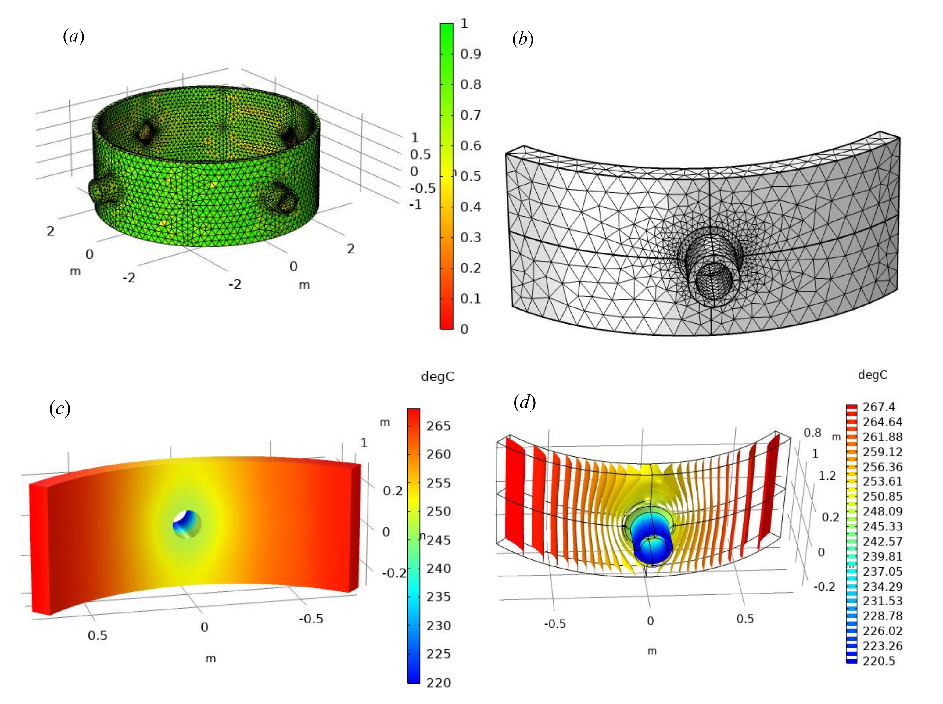
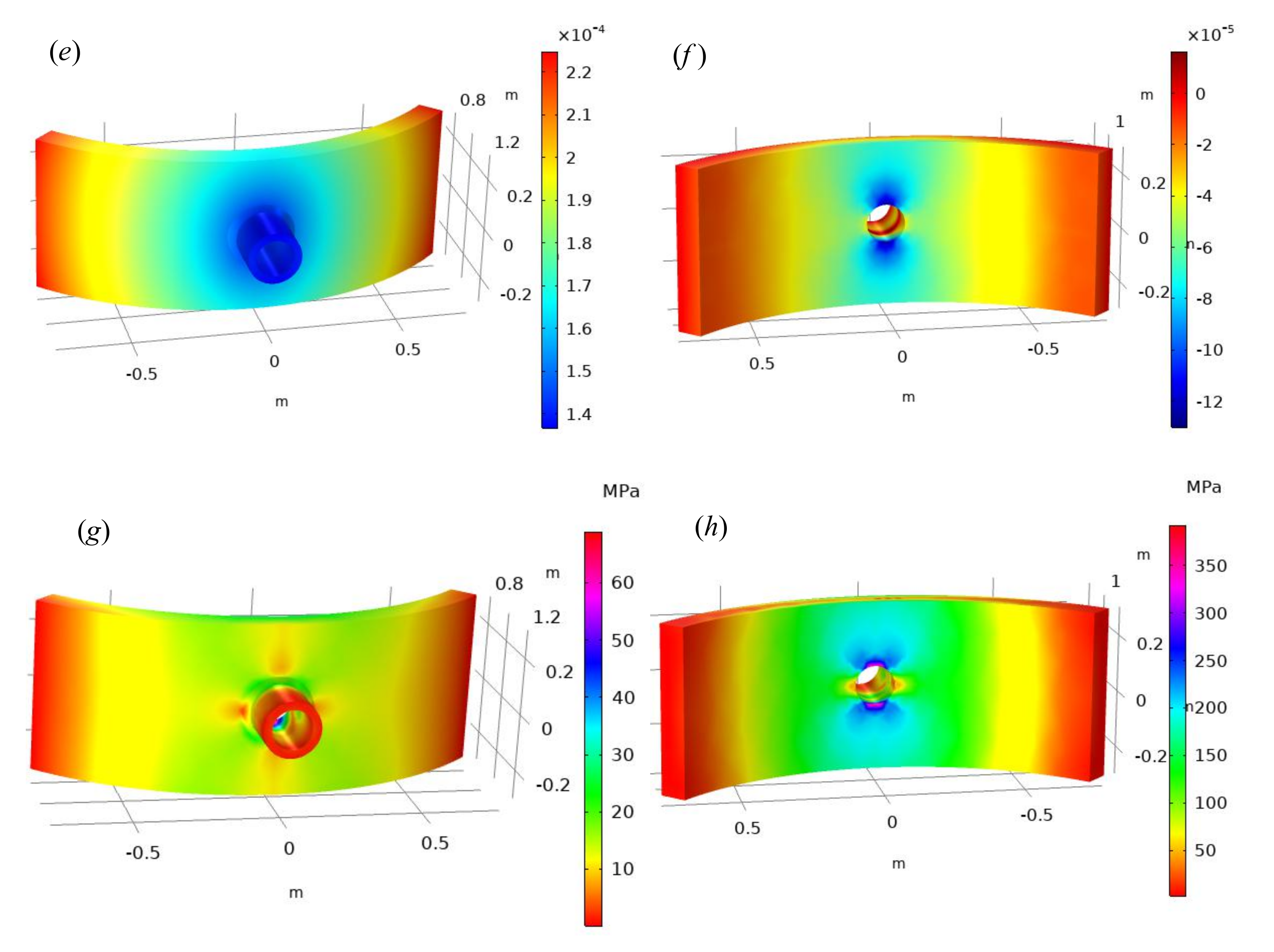
6.5. Numerical Result Display

The RPV parameters are divided into geometric parameters and basic material property parameters. For the RPV radius $R=5$ m we simulated, the wall thickness $d=15$ cm, the radius of the pipe mouth $r_{pip}=10\mathrm{cm}$, the thickness of the pipe wall $d_{pip}=4\mathrm{cm}$, and the height of the RPV calculation area $H=0.6\mathrm{m}$. This example uses tetrahedral elements, and we perform discretization. Figure 8 below shows the mesh quality evaluation diagram. This example simulates an RPV with four nozzles. The structure contains 58,910 domain elements, 30,345 boundary elements, and 3985 edge elements. The green mesh in Figure 8a indicates that the mesh quality is relatively good, and the yellow part belongs to the part with poor mesh quality. The overall quality of the mesh divided in this example is relatively good. Due to the symmetry of RPV, we only need to study the stress and temperature changes of a nozzle. Figure 8b is the result of meshing the tetrahedral element of one nozzle. The vicinity of the nozzle is the focus of our research, so the adaptive meshing method is adopted. It has a total of 9735 domain elements, 3297 boundary elements, and 471 edge elements, and the mesh has the characteristics of self-adaptation, which can not only ensure the advantages of fast calculation speed but also ensure the accurate description of the details of stress changes at the interface of the pipe wall. It can smoothly transition the numerical results of positions with large stress gradient changes, which makes the visualization effect better. The mesh quality evaluation chart shows that the mesh effect near the exhaust pipe is relatively poor, and the geometric change of the RPV container wall is gentle, so the mesh quality of the element is better.

Regarding other numerical results, Figure 8c shows the inner temperature variation diagram of the RPV nozzle at the calculation time t = 420 s, which reflects that the temperature of the nozzle is relatively lower than that of other positions. The reason is that the coolant added at the nozzle can reduce the temperature near the nozzle. Figure 8d is the isothermal line diagram of the three-dimensional nozzle. The outer side of the RPV is shown in the figure, and different colors represent different temperatures. Similarly, it can be seen from the figure that the temperature near the nozzle is relatively low, and there is a cooling effect caused by the combined action of air cooling and coolant. Figure 8e is the displacement cloud map of an RPV nozzle at t = 7200 s, which reflects the initial starting time; the force generated by the internal pressure is large, and the temporary change of the cooling system is not very obvious. Figure 8f is the strain ${\epsilon }_{xx}$ of RPV, and the change range near the nozzle is significantly larger than the change of the internal value of the nozzle. The change of strain and displacement is mainly affected by the thickness of the material, the external load, the elastic modulus of the material, the Poisson ratio, and other basic properties. The results show a comprehensive response; not only the embodiment of the load change but also the change of the displacement is significantly larger than the strain. This can also be reflected from the geometric constitutive equation.

The symmetrical geometric appearance is helpful for element calculation, and the numerical results show that the stress change is relatively large at the intersection of the pipe of the RPV. In the actual application process, the RPV is accompanied by multiple exhaust pipes, which can exhaust gas, add coolant, etc. Therefore, the third numerical model of this paper is mainly to analyze the stress change near the pipe mouth, and we have established a three-dimensional finite element model of thermal–mechanical coupling. The adaptive mesh is used to discretize the pipe mouth area. Finally, the numerical solution cloud map of the stress, strain, and displacement of the RPV pipe mouth is obtained. Then, we compared the radial and hoop stress changes of RPV at different times. The physical model established in this paper and the new numerical method proposed in this paper have important reference values for the stress analysis of RPV, and the method can also be transferred to other coupled physical models. The safe control of nuclear energy production is a meaningful research topic.

Figure 9a is the circumferential stress of the RPV vessel wall. We choose four time points: t = 1200 s, t = 2400 s, t = 3600 s, and t = 7200 s. From the curve trend, it can be seen in the initial t = 1200 s and subsequent t = 7200 s, the hoop stress is larger, mainly because the internal pressure is larger. Of course, the thermal stress formed by temperature will also have a partial influence. It should be noted that the distance from the outer surface of the RPV (d = 150 mm) will produce reverse stress on the vessel wall, which is formed by the interaction between internal stresses. Similarly, Figure 9a,b form a set of stress comparison diagrams. Figure 9b is the axial stress above the pipe mouth. The trend is basically similar to that in Figure 9a, and the stress gradually decreases. The difference is that the stress near the pipe mouth changes obviously, the gradient value is relatively large, and the other positions decrease slowly, which is mainly due to the stress concentration at the pipe mouth. This also shows that the numerical results are in good agreement with the actual situation.

7. Conclusions

The purpose of this paper is to study the stress variation of nuclear pressure vessels. The mechanical models of pressure vessels established in this paper are from one-dimensional to three-dimensional. The theory of each model and three numerical examples are given. For a one-dimensional model, the equilibrium equation is mainly established according to the internal pressure, axial stress, and circumferential stress of RPV. The model belongs to the rough estimation of stress, and the error is too large. The conclusion of the theoretical model is that the circumferential stress is twice the axial stress. In this paper, the continuous damage dynamic model with cross-section finite element method (CMMD-TCFEM) is proposed. The advantage of this model is that it can dynamically describe the change of physical parameters of RPV under the action of the loss factor. The model has the characteristics of fast calculation, layered, and localized display. The model can obtain the stress distribution cloud map of axial and radial 2D sections. The numerical conclusion is that the Poisson’s ratio increases with the increase of temperature ($\widehat{u}$,${\mathcal{E}}_{\mathrm{t}}$), and the Young’s modulus decreases with the increase of temperature ($\widehat{u},\widehat{d}$).

In the second numerical example, axisymmetric theory is mainly given. After giving the geometric parameters and material parameters, the model can output the stress and strain nephogram of RPV under different internal pressures. The other contribution is to compare the initial state of RPV and the deformation of RPV after internal pressure. Compared with the CMMD-TCFEM method, the 3D axisymmetric method can obtain the overall stress and strain cloud map, which is more complete and intuitive. The numerical results show that the stress change at both ends of RPV is significantly greater than that of the middle vessel wall, and the reinforcement method should be adopted at both ends of the RPV. In practical application, RPV is accompanied by multiple exhaust pipes to release steam and add coolant, and stress modeling and solution near the exhaust pipe are also very important. Therefore, in example 3, a three-dimensional finite element model of thermal–mechanical coupling is established, and the adaptive mesh is used to discrete the solution area. Finally, the stress, strain, displacement, and other information of the RPV pipe mouth are obtained. We also compare the changes of radial stress and circumferential stress near the RPV pipe mouth. The numerical results show that the distance d from the inner surface is from inside to outside, and the radial stress and circumferential stress near the RPV pipe mouth gradually decrease.

In short, the new numerical method proposed in this paper corresponds to a number of different models, from one-dimensional to three-dimensional, from a single physical field to a multi-physical field. The continuous damage dynamic model is successfully combined with the finite element method, which can better characterize the elastic modulus and Poisson ratio with the change of the damage factor. The axisymmetric model and the coupling model of the nozzle can provide theoretical and simulation experience for RPV design and stress simulation. Our method reflects the multidisciplinary intersection and can solve the same problem from different angles. Our future work will focus on the intelligent application of nuclear energy. It includes optimizing fuel metering and periodically automatically detecting the performance of RPV materials. Machine learning is used to predict the internal temperature of RPV in real time, and multi-scale theory is used to analyze the defects and crack propagation of RPV materials. The application of these problems will contribute to the effective improvement of nuclear technology and provide a good theoretical basis for the application and design of a new generation of nuclear energy, so that nuclear energy can better benefit mankind and create more energy value for society.

References

1. Wang, Z. Hybridized Heuristic Heterogeneous Mathematical modeling for sustainable International comparison of the economic efficiency in nuclear energy. Sustain. Energy Technol. Assess. 2022, 50, 101578. [Google Scholar] [CrossRef]
2. Niu, X.; Zhu, S.; He, J.; Ai, Y.; Shi, K.; Zhang, L. Fatigue reliability design and assessment of reactor pressure vessel structures: Concepts and validation. Int. J. Fatigue 2021, 153, 106524. [Google Scholar] [CrossRef]
3. Solazzi, L.; Vaccari, M. Reliability design of a pressure vessel made of composite materials. Compos. Struct. 2022, 279, 114726. [Google Scholar] [CrossRef]
4. Onizawa, K.; Nishikawa, H.; Itoh, H. Development of probabilistic fracture mechanics analysis codes for reactor pressure vessels and piping considering welding residual stress. Int. J. Press. Vessel. Pip. 2010, 87, 2–10. [Google Scholar] [CrossRef]
5. Kanto, Y.; Onizawa, K.; Machida, H.; Isobe, Y.; Yoshimura, S. Recent Japanese research activities on probabilistic fracture mechanics for pressure vessel and piping of nuclear power plant. Int. J. Press. Vessel. Pip. 2010, 87, 11–16. [Google Scholar] [CrossRef]
6. Chou, H.; Chang, C. Probabilistic fracture analysis for boiling water reactor vessels considering seismic loads during decommissioning transition period. Ann. Nucl. Energy 2022, 167, 108827. [Google Scholar] [CrossRef]
7. Huang, C.; Chou, H.; Chen, B.; Liu, R.; Lin, H. Probabilistic fracture analysis for boiling water reactor pressure vessels subjected to low temperature over-pressure event. Ann. Nucl. Energy 2012, 43, 61–67. [Google Scholar] [CrossRef]
8. Li, C.; Shu, G.; Liu, W.; Duan, Y. The unified model for irradiation embrittlement prediction of reactor pressure vessel. Ann. Nucl. Energy 2020, 139, 107246. [Google Scholar] [CrossRef]
9. Bhattacharyya, M.; Fau, A.; Desmorat, R.; Alameddin, S.; Néron, D.; Ladevèze, P.; Nackenhorst, U. A kinetic two-scale damage model for high-cycle fatigue simulation using multi-temporal Latin framework. Eur. J. Mech. Solids 2019, 77, 103808. [Google Scholar] [CrossRef]
10. Naumenko, K.; Gariboldi, E. Experimental analysis and constitutive modeling of anisotropic creep damage in a wrought age-hardenable Alalloy. Eng. Fract. Mech. 2022, 259, 108119. [Google Scholar] [CrossRef]
11. Yvonnet, J.; He, Q.; Li, P. A data-driven harmonic approach to constructing anisotropic damage models with a minimum number of internal variables. J. Mech. Phys. Solids 2022, 162, 104828. [Google Scholar] [CrossRef]
12. Murtaza, U.T.; Hyder, M.J. Optimization of the size and shape of the set-in nozzle for a PWR reactor pressure vessel. Nucl. Eng. Des. 2015, 284, 219–227. [Google Scholar] [CrossRef]
13. Lu, B.T.; Song, F.; Gao, M.; Elboujdaini, M. Crack growth prediction for underground high pressure gas lines exposed to concentrated carbonate–bicarbonate solution with high pH. Eng. Fract. Mech. 2011, 78, 1452–1465. [Google Scholar] [CrossRef]
14. Singh, R.; Singh, V.; Arora, A.; Mahajan, D.K. In-situ investigations of hydrogen influenced crack initiation and propagation under tensile and low cycle fatigue loadings in RPV steel. J. Nucl. Mater. 2020, 529, 151912. [Google Scholar] [CrossRef]
15. Vukojević, N.; Gubeljak, N.; Terzic, M.; Hadžikadunić, F. Analysis of the impact of position in fatigue cracks on the fracture toughness of thick-walled pressure vessel material. Procedia Struct. Integr. 2016, 2, 2982–2988. [Google Scholar] [CrossRef] [Green Version]
16. Czapski, P. Influence of laminate code and curing process on the stability of square cross-section, composite columns—Experimental and FEM studies. Compos. Struct. 2020, 250, 112564. [Google Scholar] [CrossRef]
17. Kundrák, J.; Karpuschewski, B.; Pálmai, Z.; Felhő, C.; Makkai, T.; Borysenko, D. The energetic characteristics of milling with changing cross-section in the definition of specific cutting force by FEM method. CIRP J. Manuf. Sci. Technol. 2021, 32, 61–69. [Google Scholar] [CrossRef]
18. Dodig, H. A boundary integral method for numerical computation of radar cross section of 3D targets using hybrid BEM/FEM with edge elements. J. Comput. Phys. 2017, 348, 790–802. [Google Scholar] [CrossRef]
19. Oh, C.; Lee, S.; Jhung, M.J. Analytical method to estimate cross-section stress profiles for reactor vessel nozzle corners under internal pressure. Nucl. Eng. Technol. 2022, 54, 401–413. [Google Scholar] [CrossRef]
20. Wu, X.; Wang, Z.; Fan, H.; Liu, P. Investigation on theoretical solution of geometric deformation of pressure vessel and pipe subjected to thermo-mechanical loadings. Int. J. Press. Vessel. Pip. 2021, 194, 104564. [Google Scholar] [CrossRef]
21. Moskovka, A.; Valdman, J. Fast MATLAB evaluation of nonlinear energies using FEM in 2D and 3D: Nodal elements. Appl. Math. Comput. 2022, 424, 127048. [Google Scholar] [CrossRef]
22. Hwang, J.; Kim, Y.; Kim, J. Energy-based damage model incorporating failure cycle and load ratio effects for very low cycle fatigue crack growth simulation. Int. J. Mech. Sci. 2022, 221, 107223. [Google Scholar] [CrossRef]
23. González-Albuixech, V.F.; Qian, G.; Sharabi, M.; Niffenegger, M.; Niceno, B.; Lafferty, N. Coupled RELAP5, 3D CFD and FEM analysis of postulated cracks in RPVs subjected to PTS loading. Nucl. Eng. Des. 2016, 297, 111–122. [Google Scholar] [CrossRef]
24. González-Albuixech, V.F.; Qian, G.; Sharabi, M.; Niffenegger, M.; Niceno, B.; Lafferty, N. Comparison of PTS analyses of RPVs based on 3D-CFD and RELAP5. Nucl. Eng. Des. 2015, 291, 168–178. [Google Scholar] [CrossRef]
25. Chouhan, R.; Kansal, A.K.; Maheshwari, N.K.; Sharma, A. Computational studies on pressurized thermal shock in reactor pressure vessel. Ann. Nucl. Energy 2021, 152, 107987. [Google Scholar] [CrossRef]
26. Chen, M.; Yu, W.; Qian, G.; Shi, J.; Cao, Y.; Yu, Y. Crack initiation, arrest and tearing assessments of a RPV subjected to PTS events. Ann. Nucl. Energy 2018, 116, 143–151. [Google Scholar] [CrossRef]
27. Huang, P.; Chou, H.; Ferng, Y.; Kang, C. Large thermal gradients on structural integrity of a reactor pressure vessel subjected to pressurized thermal shocks. Int. J. Press. Vessel. Pip. 2020, 179, 103942. [Google Scholar] [CrossRef]
28. Sun, X.; Lu, W.; Chai, G.; Bao, Y. Effect of cladding thickness on brittle fracture prevention of the base wall of reactor pressure vessel. Thin-Walled Struct. 2021, 158, 107163. [Google Scholar] [CrossRef]
29. Christian, R.; Lee, Y.; Kang, H.G. Emergency core cooling system performance criteria for Multi-Layered Silicon Carbide nuclear fuel cladding. Nucl. Eng. Des. 2019, 353, 110280. [Google Scholar] [CrossRef]
30. Wang, J.; Zhang, L.; Qu, J.; Tong, J.; Wu, G. Rapid accident source term estimation (RASTE) for nuclear emergency response in high temperature gas cooled reactor. Ann. Nucl. Energy 2020, 147, 107654. [Google Scholar] [CrossRef]
31. Oliver, S.; Simpson, C.; Collins, D.M.; Reinhard, C.; Pavier, M.; Mostafavi, M. In-situ measurements of stress during thermal shock in clad pressure vessel steel using synchrotron X-ray diffraction. Int. J. Mech. Sci. 2021, 192, 106136. [Google Scholar] [CrossRef]
32. Zhao, P.; Ji, K.; Zhang, J.; Chen, Y.; Dong, Z.; Zheng, J.; Fu, J. In-situ ultrasonic measurement of molten polymers during injection molding. J. Mater. Process. Technol. 2021, 293, 117081. [Google Scholar] [CrossRef]
33. Tasavori, M.; Maleki, A.T.; Ahmadi, I. Composite coating effect on stress intensity factors of aluminum pressure vessels with inner circumferential crack by X-FEM. Int. J. Press. Vessel. Pip. 2021, 194, 104445. [Google Scholar] [CrossRef]
34. Zhang, K.; Sanchez-Espinoza, V.H. The Dynamic-Implicit-Additional-Source (DIAS) method for multi-scale coupling of thermal-hydraulic codes to enhance the prediction of mass and heat transfer in the nuclear reactor pressure VESSEL. Int. J. Heat Mass Transf. 2020, 147, 118987. [Google Scholar] [CrossRef]
35. Huo, Y.; Yu, H.; Wang, M.; Tian, W.; Qiu, S.; Su, G.H. Development and application of TaSNAM 2.0 for advanced pressurized water reactor. Ann. Nucl. Energy 2022, 166, 108801. [Google Scholar] [CrossRef]
36. Mackerle, J. Finite elements in the analysis of pressure vessels and piping—A bibliography (1976–1996). Int. J. Press. Vessel. Pip. 1996, 69, 279–339. [Google Scholar] [CrossRef]
37. Mohanavel, V.; Prasath, S.; Arunkumar, M.; Pradeep, G.M.; Babu, S.S. Modeling and stress analysis of aluminium alloy based composite pressure vessel through ANSYS software. Mater. Today Proc. 2021, 37, 1911–1916. [Google Scholar] [CrossRef]
38. You, Q.; Mo, N.; Liu, X.; Luo, H.; Shi, Z. Experiments on helium breakdown at high pressure and temperature in uniform field and its simulation using COMSOL Multiphysics and FD-FCT. Ann. Nucl. Energy 2020, 141, 107351. [Google Scholar] [CrossRef]
39. Yang, Z.; Liu, H. A continuum fatigue damage model for the cyclic thermal shocked ceramic-matrix composites. Int. J. Fatigue 2020, 134, 105507. [Google Scholar] [CrossRef]
40. Damhof, F.; Brekelmans, W.A.M.; Geers, M.G.D. Non-local modeling of thermal shock damage in refractory materials. Eng. Fract. Mech. 2008, 75, 4706–4720. [Google Scholar] [CrossRef]
41. Zhu, C.; Li, Y.; Tan, H.; Shi, J.; Nie, Y.; Qiu, Q. Multi-field coupled effect of thermal disturbance on quench and recovery characteristic along the hybrid energy pipe. Energy 2022, 246, 123362. [Google Scholar] [CrossRef]
42. Lemaitre, J.; Chaboche, J.L.; Maji, A.K. Mechanics of Solid Materials. J. Eng. Mech. 1992, 119, 642–643. [Google Scholar] [CrossRef]
43. Almasi, A.; Baghani, M.; Moallemi, A. Thermomechanical analysis of hyperelastic thick-walled cylindrical pressure vessels, analytical solutions and FEM. Int. J. Mech. Sci. 2017, 130, 426–436. [Google Scholar] [CrossRef]
44. Yang, Z.; Lui, H. A continuum damage mechanics model for 2-D woven oxide/oxide ceramic matrix composites under cyclic thermal shocks. Ceram. Int. 2020, 46, 6029–6037. [Google Scholar] [CrossRef]
45. Yang, Y.; Schiavone, P.; Li, X. Effect of surface elasticity on transient elastic field around a mode-III crack-tip under impact loads. Eng. Fract. Mech. 2021, 258, 108062. [Google Scholar] [CrossRef]
46. Chen, W.; Dai, S.; Zheng, B. ARIMA-FEM Method with Prediction Function to Solve the Stress-Strain of Perforated Elastic Metal Plates. Metals 2022, 12, 179. [Google Scholar] [CrossRef]
47. Demirbas, M.D. Thermal stress analysis of functionally graded plates with temperature-dependent material properties using theory of elasticity. Engineering 2017, 131, 100–124. [Google Scholar] [CrossRef]
48. Li, C.; Guo, H.; Tian, X.; He, T. Time-domain finite element method to generalized diffusion-elasticity problems with the concentration-dependent elastic constants and the diffusivity. Appl. Math. Model. 2020, 87, 55–76. [Google Scholar] [CrossRef]
49. Si, H.M.; Cho, C.; Kwahk, S.Y. A hybrid method for casting process simulation by combining FDM and FEM with an efficient data conversion algorithm. J. Mater. Process. Technol. 2003, 133, 311–321. [Google Scholar] [CrossRef]
50. Zhang, H.; Tong, L.; Addo, M.A.; Liang, J.; Wang, L. Research on contact algorithm of unbonded flexible riser under axisymmetric load. Int. J. Press. Vessel. Pip. 2020, 188, 104248. [Google Scholar] [CrossRef]
51. Que, Z.; Seifert, H.P.; Spätig, P.; Zhang, A.; Holzer, J.; Rao, G.S.; Ritter, S. Effect of dynamic strain ageing on environmental degradation of fracture resistance of low-alloy RPV steels in high-temperature water environments. Corros. Sci. 2019, 152, 172–189. [Google Scholar] [CrossRef]
52. Li, Y.; Jin, T.; Wang, Z.; Wang, D. Engineering critical assessment of RPV with nozzle corner cracks under pressurized thermal shocks. Nucl. Eng. Technol. 2020, 52, 2638–2651. [Google Scholar] [CrossRef]
53. Sun, X.; Chai, G.; Bao, Y. Ultimate bearing capacity analysis of a reactor pressure vessel subjected to pressurized thermal shock with XFEM. Eng. Fail. Anal. 2017, 80, 102–111. [Google Scholar] [CrossRef]
54. Bao, W.; Garcke, H.; Nürnberg, R.; Zhao, Q. Volume-preserving parametric finite element methods for axisymmetric geometric evolution equations. J. Comput. Phys. 2022, 460, 111180. [Google Scholar] [CrossRef]
55. Li, Q.; Hou, P.; Shang, S. Accurate 3D thermal stress analysis of thermal barrier coatings. Int. J. Mech. Sci. 2022, 217, 107024. [Google Scholar] [CrossRef]
56. Upadhyay, K.; Subhash, G.; Spearot, D. Hyperelastic constitutive modeling of hydrogels based on primary deformation modes and validation under 3D stress states. Int. J. Eng. Sci. 2020, 154, 103314. [Google Scholar] [CrossRef]
57. Zhou, F.; You, Y.; Li, G.; Xie, G.; Li, G. The precise integration method for semi-discretized equation in the dual reciprocity method to solve three-dimensional transient heat conduction problems. Eng. Anal. Bound. Elem. 2018, 95, 160–166. [Google Scholar] [CrossRef]
58. Wu, Q.; Peng, M.J.; Fu, Y.D.; Cheng, Y.M. The dimension splitting interpolating element-free Galerkin method for solving three-dimensional transient heat conduction problems. Eng. Anal. Bound. Elem. 2021, 128, 326–341. [Google Scholar] [CrossRef]
59. Zhang, H.; Yang, Y.; Huang, W. Influence of the thermal insulation layer on radial stress and collapse resistance of subsea wet insulation pipe. Ocean Eng. 2021, 235, 109374. [Google Scholar] [CrossRef]
60. Chen, W.; Dai, S.; Zheng, B.; Lin, H. An Efficient Evaluation Method for Automobile Shells Design Based on Semi-supervised Machine Learning Strategy. J. Phys. Conf. Ser. ICCBD2021 2022, 2171, 012026. [Google Scholar] [CrossRef]
61. Duru, K.L.; Rannabauer, L.; Gabriel, A.; Ling, O.K.A.; Igel, H.; Bader, M. A stable discontinuous Galerkin method for linear elastodynamics in 3D geometrically complex elastic solids using physics based numerical fluxes. Comput. Methods Appl. Mech. Eng. 2022, 389, 114386. [Google Scholar] [CrossRef]
62. Yalameha, S.; Nourbakhsh, Z.; Vashaee, D. ElATools: A tool for analyzing anisotropic elastic properties of the 2D and 3D materials. Comput. Phys. Commun. 2022, 271, 108195. [Google Scholar] [CrossRef]
63. Xu, F.; Liu, Q.; Shibahara, M. Transient and steady-state heat transfer for forced convection of helium gas in minichannels with various inner diameters. Int. J. Heat Mass Transf. 2022, 191, 122813. [Google Scholar] [CrossRef]
64. Solin, P.; Dubcova, L.; Kruis, J. Adaptive hp-FEM with dynamical meshes for transient heat and moisture transfer problems. J. Comput. Appl. Math. 2010, 12, 3103–3112. [Google Scholar] [CrossRef] [Green Version]
65. Erath, C.; Gantner, G.; Praetorius, D. Optimal convergence behavior of adaptive FEM driven by simple-type error estimators. Comput. Math. Appl. 2020, 79, 623–642. [Google Scholar] [CrossRef] [Green Version]
66. Bériot, H.; Gabard, G. Anisotropic adaptivity of the p-FEM for time-harmonic acoustic wave propagation. J. Comput. Phys. 2019, 378, 234–256. [Google Scholar] [CrossRef]
67. Giani, S.; Solin, P. Solving elliptic eigenproblems with adaptive multimesh hp-FEM. J. Comput. Appl. Math. 2021, 394, 113528. [Google Scholar] [CrossRef]
Figure 1. Development history of main metal elements of RPV in China.
Fractalfract 06 00215 g001
Figure 2. Working principle diagram of the pressurized water reactor nuclear power plant.
Fractalfract 06 00215 g002
Figure 3. Ilustration of the internal structure and important parts of the pressure vessel.
Fractalfract 06 00215 g003
Figure 4. Stress estimation of capsule shaped nuclear pressure vessel. (a) Hoop stress of RPV. (b) Axial stress of RPV.
Fractalfract 06 00215 g004
Figure 5. Variation of internal parameters of pressure vessel with temperature in structural damage dynamic model. (a) Variation trend of internal temperature and pressure of RPV with time t. (b) Variation diagram of Young’s modulus and temperature. (c) Young’s modulus for solving damage dynamic model of continuous structure. (d) Comparing the Possion rate v of the traditional model with the damage model.
Fractalfract 06 00215 g005aFractalfract 06 00215 g005b
Figure 6. The axial stress and radial stress of RPV are solved by FEM combined with the damage dynamic model. (a) The diagram of inner load on a axial section. (b) The diagram of inner load on a radial section. (c) The axial section stress τ x y diagram of RPV. (d) The axial section stress σ x x diagram of RPV. (e) The Von Mises stress of radial section of RPV. (f) The strain ε x x of radial section of RPV.
Fractalfract 06 00215 g006
Figure 7. Numerical results of mechanical change of RPV solved by axisymmetric FEM. (a) Deformation diagram of the symmetrical half-section of the pressure vessel at F = 15.2 Mpa. (b) The radial strain ε r r cloud diagram of the pressure vessel at F = 13 Mpa. (c) von Mises stress nephogram of the pressure vessel at F = 3 Mpa. (d) von Mises stress nephogram of the pressure vessel at F = 16.8 Mpa.
Fractalfract 06 00215 g007
Figure 8. Numerical simulation of RPV by 3D thermal-mechanics coupled model. (a) Mesh quality assessment of all pipe outlets. (b) 4-NQ element grid division of RPV single pipe outlet and adjacent area. (c) Temperature T nephogram of RPV pipe mouth. (d) Isothermal line diagram of RPV pipe mouth. (e) Displacement of RPV nozzle U. (f) Strain ε x x nephogram near RPV nozzle. (g) Von Mises stress of RPV pipe. (h) Stress nephogram of σ y y .
Fractalfract 06 00215 g008aFractalfract 06 00215 g008b
Figure 9. Variation trend of radial stress and circumferential stress of RPV with calculation distance. (a) Hoop stress on the RPV wall. (b) Axial stress above the nozzle.
Fractalfract 06 00215 g009