1. Introduction
Advancements in the understanding of heart functioning and related mechanisms have contributed to the progress and development of more appropriate clinical and surgical treatments of heart diseases [
1]. In spite of the progress, these conditions are composed of complex phenomena, thus figuring as a multidisciplinary challenge that demands contribution from not only medical sciences professionals, but also researchers of different knowledge areas, such as mathematicians, physicists, engineers, among others [
2].
The heart consists mainly of muscle, with their cells collectively being called myocardium. There are two types of heart cell. Known as muscle fibers, the first type corresponds to muscle cells which have a contractile function that plays the mechanical role of contraction. The second type refers to specialized cells that start the heart rhythm and propagate electrical impulses, coordinating this activity [
3].
In order to exercise the mechanical function of pumping blood, myocardial cells need to be activated by an electrical stimulus that acts on the cell membrane. This electrical action is caused by the movement of ions through cell membranes. It is known that the intra- and extracellular potentials and the currents established by the ion flows through the cardiac membrane are important electrical variables to study cardiac tissue conduction [
4]. Moreover, the mechanical motions of the heart are stimulated and coordinated by electrical waves that originate in the region of the sinoatrial node and spread through the atria and ventricles, each different one being responsible for distinct progressions of cardiac impulses [
5,
6].
Physical descriptions of these processes can be elaborated through the knowledge of meticulous macroscopic and microscopic voltage clamping measures at the level of individual ion channels. The ionic models that describe cardiac action potential have become increasingly complex. This complexity, when translated to mathematical models, makes it difficult to isolate sets of parameters essential to understanding the system.
According to recent literature, new models have been proposed to study and simulate the electrical activities of the heart. In most of them, it is not necessary to model the ionic currents of the cell with the precision and complexity inherent to biophysics-based models. Instead, more simplified approaches have been investigated. Accordingly, mathematical modeling and computer simulation of cardiac tissue conduction frameworks have allowed not only qualitative analysis, but also to access to relevant quantitative information about the related phenomena.
Accordingly, in the context of mathematical prediction [
7], optimal control [
8], and stability of stationary solutions [
9,
10], fractional calculus modeling [
11,
12,
13] has recently been adopted to describe biological and health-related processes, particularly the dynamics of cardiac phenomena [
14,
15,
16,
17]. In general, the results achieved by those papers indicated that fractional models can detect subtleties when compared to their counterparts. While there is a continuous debate on which derivatives are better suited for distinct applications [
18] and on their physical and geometrical interpretations, including the concept of memory [
19], fractional calculus has proven useful in several different areas of application. Therefore, our interest in modeling action potential phenomena in cardiac tissue using non-integer-order derivatives stemmed from breakthroughs and significant results from those and other works regarding biological tissue modeling under fractional calculus.
As a remarkable example, Magin explored fractional models to describe the complex dynamics of biological tissue. Since tissue properties come from materials’ nanoscale and microscale organization, he proposed that dynamic models could predict macroscale tissue behavior and fractional calculus would play an important role in describing these events through concise and effective models [
17]. In parallel, Meral and colleagues offered experimental evidence that fractional differential equations could model tissue-like soft and porous materials better under a viscoelastic framework [
20].
In relation to heart-related tissue, its solid and fluidlike composition make it suitable for modeling through the assessment of viscoelastic properties. In this context, a generalized fractional-order Maxwell model successfully predicted the behavior of atrial tissue compared to experimental data [
21]. Moreover, there is evidence pointing towards a better description of phenomena concerning impulse propagation in cardiac muscle. Due, indeed, to this high heterogeneity of such tissue, fractional diffusion models have been proposed for modeling such phenomena [
15].
In this specific context, the heterogeneous structure of cardiac tissue can be approached as an underlying fractal process. Complex-order derivates were proposed as a modeling option, where the real part represents the fractal dimension and the imaginary part corrects said dimension. The combined effect of these components seems to allow the depiction of a wide range of eletrophysiological conditions [
22]. As another possible tool, image analysis has been employed along with fractal dimension to provide a quantitative picture of myocardial fibrosis in mice [
23].
Accordingly, the strong relation between fractional calculus and fractals has been long-debated and explored, with regards to whether this fractance refers to space (as in a complex geometry) or time (with heterogeneity and memory effects) [
24]. Part of this relation is usually explored through physical and geometrical considerations with the intent of describing and predicting complex phenomena (such as physiology-related ones) [
25].
Furthermore, Butera and Di Paola have shown that once a physical phenomenon takes place in an underlying fractal geometry (such is the case for cardiac tissue), a power law naturally appears to govern its evolution, with its order directly related to the anomalous dimension of such geometry [
26] or, as commented before, to heterogeneous memory effects [
24]. For that reason, the physical meaning of magnitudes seen in this work and the order
could in turn concern the spatiotemporal fractance of the tissue wherein the phenomenon is occurring and the degree to which it interferes with how electricity diffuses in it. Hence, in this sense, the physical relevance of said units is maintained and its magnitude is only parametrized by the fractional order [
27].
Bearing in mind the importance of better understanding the dynamics of the action potential in cardiac tissues, we investigate a class of fractional time-partial differential equations capable of modeling some stages of this phenomenon. We expect that the fractional time-derivative operator can act as an additional resource in the modulation of the phenomena. Based on this class of equations, the main motivation of this paper is devoted to solving them analytically, considering both one- and two-dimensional cases. Additionally, in order to provide a better perspective and scope, we also present some numerical simulations.
Finally, the paper is organized as follows. In
Section 2, preliminaries are presented. In
Section 3, the model is introduced and the necessary mathematical development is exhibited. In
Section 4, some numerical simulations are conducted and their results are discussed. Finally, in
Section 5, the main conclusions are outlined.
2. Preliminaries
The fractional-time reaction–diffusion equation has been studied in the literature and there are a large number of papers devoted to the study of different physical phenomena applying this equation [
28,
29,
30]. Some researchers have used the Riemann–Liouville derivative [
31,
32], while others have adopted the Caputo derivative [
33,
34]—also referred as the Gerasimov–Caputo derivative [
35,
36,
37,
38]. Furthermore, different methods have been employed to solve it, such as Green’s function method [
39], finite sine transform method [
40], Fourier–Laplace transform method [
29], Adomian decomposition method [
41], and the separation of variables method introduced by Metzler et al. [
42].
This paper addresses with homogeneous and nonhomogeneous fractional-time reaction–diffusion equations and their analytical solutions are achieved by means of the separation of variables method. In this context, this section recalls fundamental concepts, definitions, and theorems, while introducing some notations that are relevant to the subsequent development of the paper. In the next section, both positioning and problem statement are presented.
Definition 1. A real function , is said to be in space , if there is a real number , such as where .
Definition 2. A real function is said to be in space , , if .
Definition 3. Mittag–Leffler function [43,44] is defined asand we note that . Definition 4 ([
45,
46])
. The two-dimensional Laplacian defined with zero Dirichlet boundary condition at , b, , c has a complete set of orthonormal eigenfunctions corresponding to eigenvalues on a boundary region .If , then the two-dimensional Laplacian has eigenvaluesand corresponding eigenfunction Proposition 1. Let be a limited domain that defines the following function space in :with and subspace of , which consists of functions whose m-order partial derivatives are uniformly continuous. Let us also consider and and define: The solution ofis given by Indeed, assuming that solves (2), and using Green’s second identity, it is possible to verify [47] that is the eigenfunction corresponding to eigenvalue . Since u is uniformly continuous and hence uniformly bounded on its domain, we have by dominated convergence that Proof. Supposing that
is the solution of Equation (
2). By coupling it to the referred partial differential equation, one obtains
so that
Therefore, to find the solution for Equation (
2), one must solve
One can notice that Equation (
3) yields
Furthermore, the autovalue problem in Equation (
4) may be solved by means of an infinite pair series (
),
, where
is a sequence of functions that form a complete orthonormal set in the considered domain. Hence, the function
can be represented as
where
is chosen to satisfy the initial condition of the considered problem.
Therefore, if
, then
For details, one may refer to [
48]. □
Proposition 2. ([
49])
. An analytical solution of problem (6) will be attempted by means of the separation of variables method. We first solve the corresponding homogeneous equation (by making the source term in (6) null). Let be the solution of the corresponding homogeneous equation in (6). We obtain a fractional ordinary differential equation for and two ordinary second-order differential equations for and for with their boundary conditions.The fractional ordinary differential equation can be integrated and its solution requires the Mittag–Leffler function. To obtain the solution of second-order equations, let also be the eigenvalues (or the separation constant).
According to Definition 4, the Sturm–Liouville problem has eigenvaluesand corresponding eigenfunctions Afterwards, we seek a solution of the nonhomogeneous problem (6) of the form We assume that the series can be differentiated term-by-term. In order to determine , we expand the function as two Fourier series by the eigenfunction . Since satisfies the initial conditions, we can apply them and hence we obtain an analytical solution of problem (6). 3. Mathematical Model
This section deals with homogeneous and non-homogeneous fractional differential equations by considering the dynamics of the action potential in cardiac tissue involving both unidimensional (1-D) and bidimensional (2-D) spatial analysis.
The mathematical model of the 2-D action potential in cardiac tissue with membrane potential
proposed in this work is governed by the following fractional partial-time differential equation (see [
50,
51,
52,
53,
54])
where
defines the potential of the membrane at location
and time
t,
k denotes a constant coefficient. The terms
and
represent the membrane tissue capacitance and ionic electric currents involved in the process, respectively. They work as a sink term in the dynamic model and were inspired in the Beeler–Reuter model [
51,
52,
53,
54].
If
is the Laplace operator and
then Equation (
5) takes the form
Equation (
6) is a type of fractional diffusion-wave equation that has been widely used in many branches of science and engineering. The time-fractional diffusion-wave equation is obtained from the classical diffusion or wave equation by replacing the first- or second-order time derivative by a fractional derivative of order
with
or
, respectively.
In accordance with the exposed definitions, the solution of a fractional differential equation can be obtained from the solution of the corresponding homogeneous equation subject to initial conditions added to a particular solution of Equation (
6). In the follow-up, a particular function characterizing a nonhomogeneous fractional 1-D differential equation is considered. Afterwards, the 2-D case is also solved for both homogeneous and nonhomogeneous case.
3.1. Fractional Differential Equation (1-D)
For the sake of clarity, we begin with the fractional 1-D and homogeneous case. Physically, this case occurs whenever has a sufficiently small value and, in turn, the value is not insignificant. In those cases, the function is closer to zero and it can be neglected.
3.1.1. Homogeneous Case
The fractional unidimensional and homogeneous case
with
,
and
k a constant is evaluated along boundary conditions given by
,
and
.
In order to apply the separation of variables method, we assume that
. Thus, one can write
The two ordinary differential equations obtained from Equation (
8) have the following solutions, respectively
where
denotes the Mittag–Leffler function and
and
A are constant.
After applying the aforementioned boundary conditions, one can obtain the final solution given by
3.1.2. Nonhomogeneous Case
In the follow-up, this section deals with fractional unidimensional and nonhomogeneous case represented by
with
,
and
k a constant subject to the same boundary conditions considered in previous
Section 3.1.1, i.e.,
,
and
. Function
is assumed to be a continuous function of
t.
The solution of the homogeneous equation associated with (
11) was obtained in
Section 3.1.1 and shown by Equation (
10). It can be rewritten as
where
.
Assuming that Equation (
12) can be differentiated term-by-term and by observing Equation (
11), one can note that
The coefficients in both sine series, i.e., on the left and right side of Equation (
13), should be the same so that
If we use the initial condition
, then
which yields
where
are Fourier coefficients.
For each value of
, Equations (
14) and (
16) make up a fractional value problem and hence,
Substituting Equations (
16) and (
17) in (
12), one can write the final solution,
3.2. Fractional Differential Equation (2-D)
This section presents the solution of Equation (
6) in two-dimensional space, i.e., in the bounded domain
of spatial variables
and time variable
t for both homogeneous and nonhomogeneous cases.
3.2.1. Homogeneous Case
We first solve the corresponding homogeneous equation of (
6), together with the boundary conditions, by using the separation of variables method. Let
be the solution of the associated homogeneous equation of (
6), i.e, the solution of Equation (
6) when we consider
.
In other words, we search the solution of the equation
with
, and
, subject to the following conditions:
Substituting
in Equation (
19), we obtain
where
A is a constant.
Consequently, we have two ordinary differential equations in the space variables
x and
y, and one fractional order differential equation in the time variable
t so that
The solutions of Equation (
22) are given, respectively, by:
where again
denotes the Mittag–Leffler function.
Therefore,
is the general solution of Equation (
19).
By applying the first four conditions of (
20) and using the superposition principle, one can write
Now, by applying the last conditions of (
20), one can obtain the Fourier coefficient given by
Therefore, the final solution for the homogeneous equation can be written as
3.2.2. Nonhomogeneous Case
Since Equation (
6) is nonhomogeneous, in this subsection, we search its analytical solution. One can note that the corresponding homogeneous Equation (
19) has a solution given by (
27) obtained in
Section 3.2.1, which can be rewritten as
where
.
Once again, assuming that Equation (
28) can be differentiated term-by-term, and by observing that the nonhomogeneous term in Equation (
5) is represented by the function
, one can write
Hence, taking into account the orthogonality relations, one can also write that
From Equations (
26) and (
30), we obtain
Therefore, substituting Equations (
26) and (
31) in Equation (
28), one can obtain the final solution.
4. Numerical Simulations
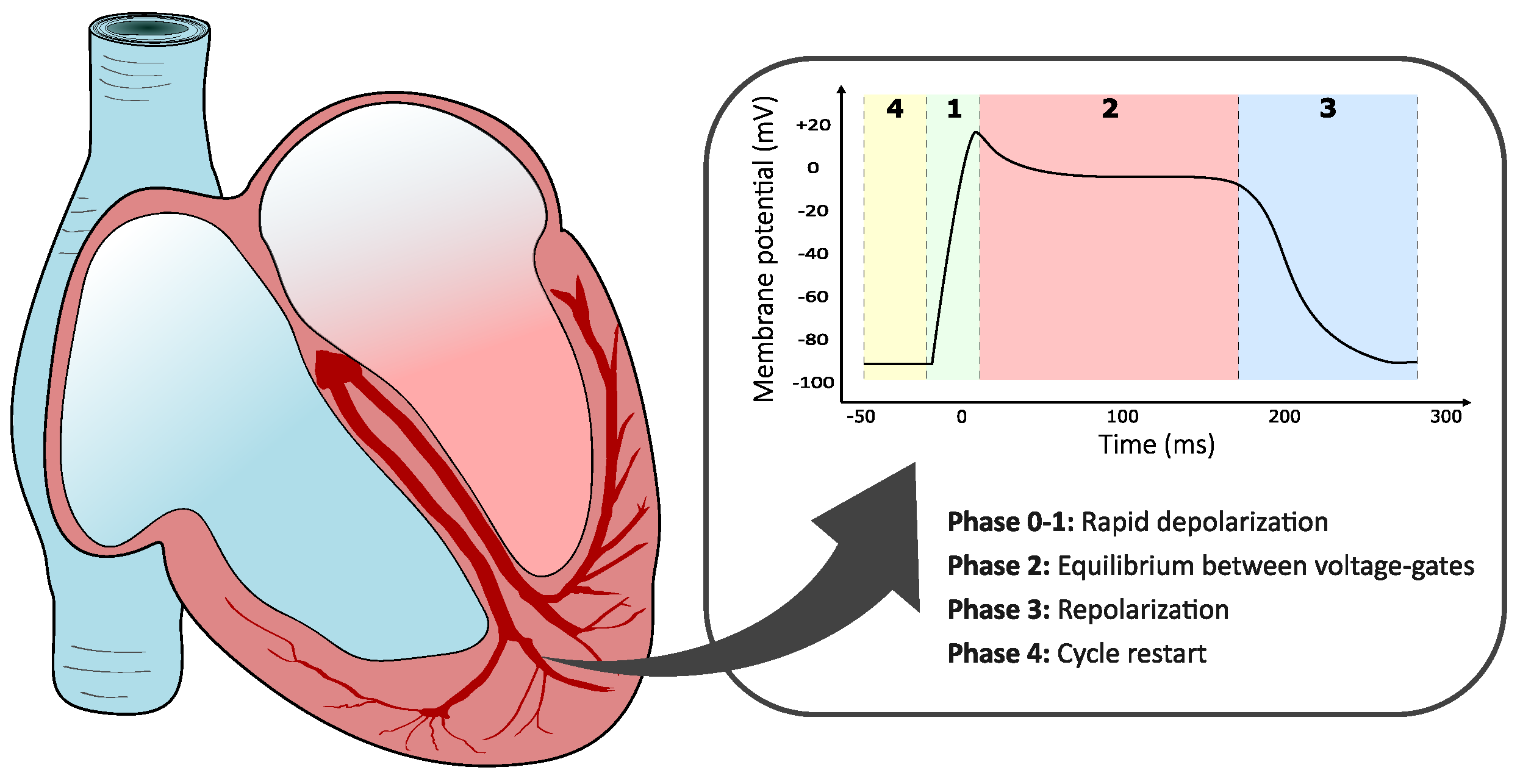
In this section, numerical simulations are presented which aim at the virtualization of hypothetical scenarios involving the potential membrane of cardiac tissues, herein modeled by the derived analytical solutions. All simulations were conducted using the software Mathematica, version 12. Integrals, special functions (such as Mittag–Leffler), and sums were numerically solved using the standard configurations in the built-in tools of the aforementioned software, which include black-box algorithms to identify and implement the fastest and most reliable numerical schemes for each integral and summations. In this context,
Figure 1 presents a scheme illustrating the typical fast response of action potential in contractile myocytes.
Overall, Phases 0 and 1 depict a quick depolarization where the membrane potential rapidly rises from around −90 mV, which is the rest potential, to the peak value of 20 mV (effectively starting muscle contraction). Next, the much longer Phase 2 represents a slight drop in potential followed by an almost entirely neutral potential due to equilibrium between calcium and potassium channels (plateau). Phase 3 concerns the start of cardiac muscle relaxation when calcium channels close and potassium channels open again, causing repolarization just before the restart of the cycle at Phase 4 [
55].
In order to explore different possibilities while still employing most of the obtained solutions, three different scenarios are suggested: (i) 1-D homogeneous; (ii) 1-D nonhomogeneous; and (iii) 2-D homogeneous dynamics. The idea here is that each of these scenarios modeled through fractional derivatives may correctly describe the behavior of at least some parts of the action potential process. The time domain analyzed in each numeric simulation depends on the duration of the particular phase being modeled.
4.1. 1-D Homogeneous Case
In this scenario, the length of cardiac tissue simulated is generically chosen as 1 mm, imposing the spatial domain as
mm. We assume that at the moment
, the considered 1-D system is starting muscle contraction, i.e., immediately at the transition between Phases 0 and 1 in the membrane potential process, after a rapid depolarization caused by opening of voltage-gated fast sodium channels (refer to
Figure 1).
In relation to the initial electrical spatial distribution, we assume that the central point
mm of our domain is where the highest membrane potential occurs. This is also referred to as peak point and is approximately 20 mV for the action potential process, occurring at the Phase 0–1 transition [
55,
56]. An initial condition
mV is therefore suggested to describe the phenomena at this point, with the sinusoidal function added to provide a gradual distribution of electricity throughout the tissue.
Referred to as myocardium diffusivity, the parameter
k refers to the capacity of the cardiac tissue to conduct or diffuse electricity during the action potential process, admitting that the phenomenon occurs homogeneously throughout space and time. In [
57], the authors conduct an extensive ECG analysis in order to characterize this and other diffusivity parameters though machine learning techniques. Although it can vary significantly from patient to patient, the authors used the equivalent to
mm
2/ms as a reference value for several tests, thus guiding our choice for this parameter value.
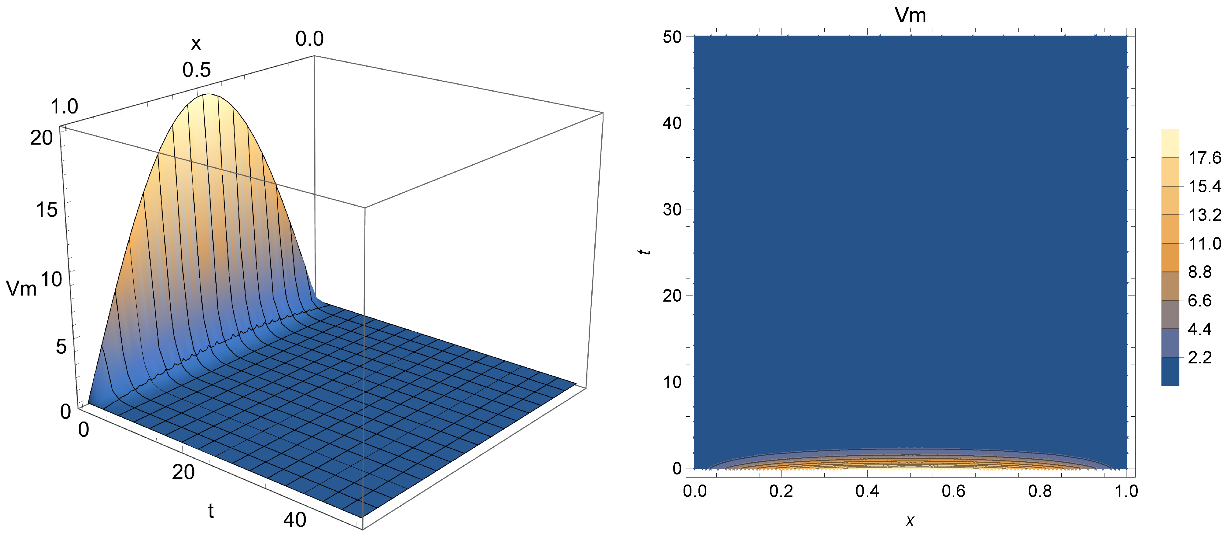
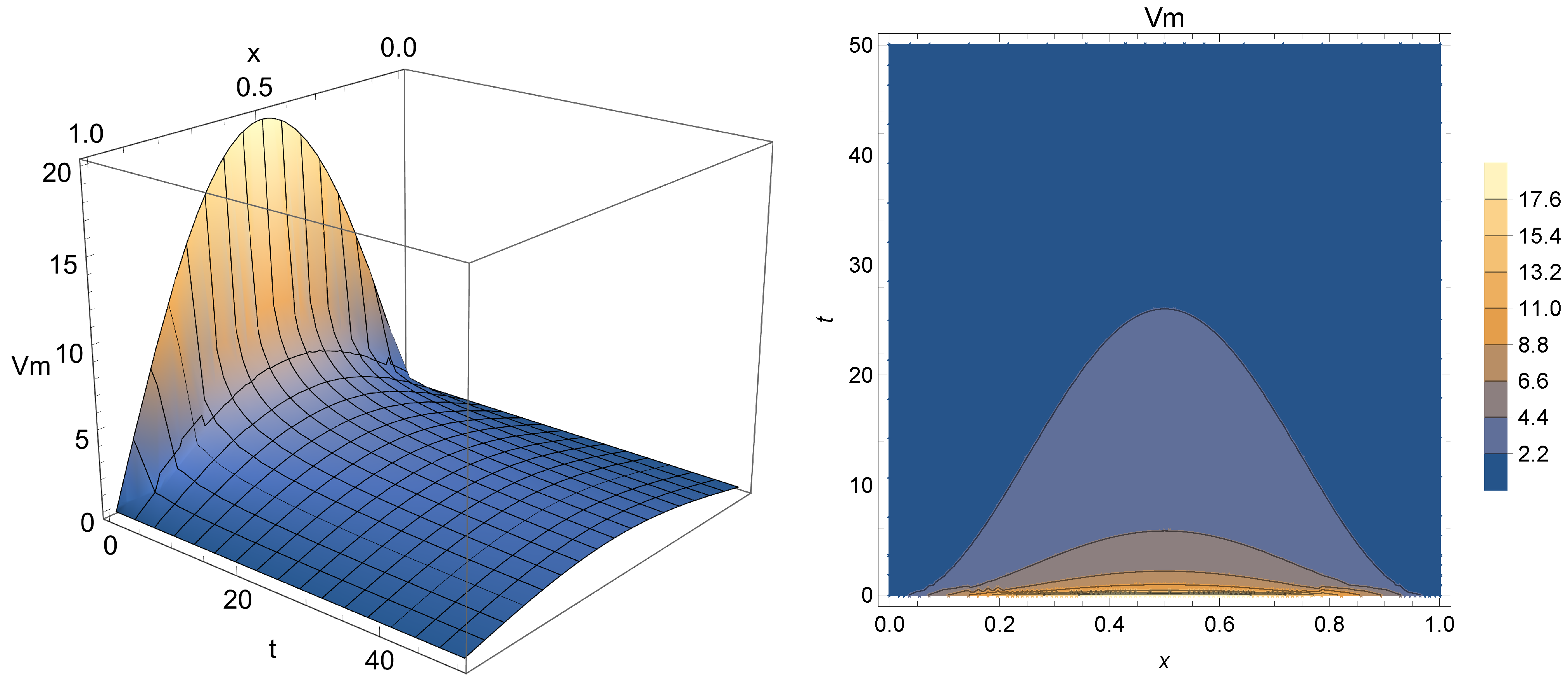
Figure 2,
Figure 3 and
Figure 4 present the results after the depolarization scenario modeled through Equation (
10) for
(i.e. traditional case),
, and
, respectively. This refers to the drop in potential through the first moments of Phase 2, just after the peak point. One can notice from the obtained results that the surface formed by the solution agree with the expected behavior of Phase 2 depolarization (i.e., a plateau caused by the opening of calcium channels and partial closure of those that admit potassium exchange). The results also show that the fractional order
enables the model to admit an extra degree of freedom compared to the traditional approach. This additional parameter may be used to control the drop in membrane potential from Phase 1, thus acting as modulator or “turning knob” for the model, with a slower electric conduction for smaller values of
, thus potentially allowing a more refined phenomenon modeling or even the description of other types of cardiac impulse (e.g., sinoatrial or atrial progressions). In fact, as the simulation covers the first 50 ms after the point of peak potential, smaller values of
seem to enable a better description of this part of the process, since
depicts a sudden drop in potential, which does not seem to be the case considering
Figure 1.
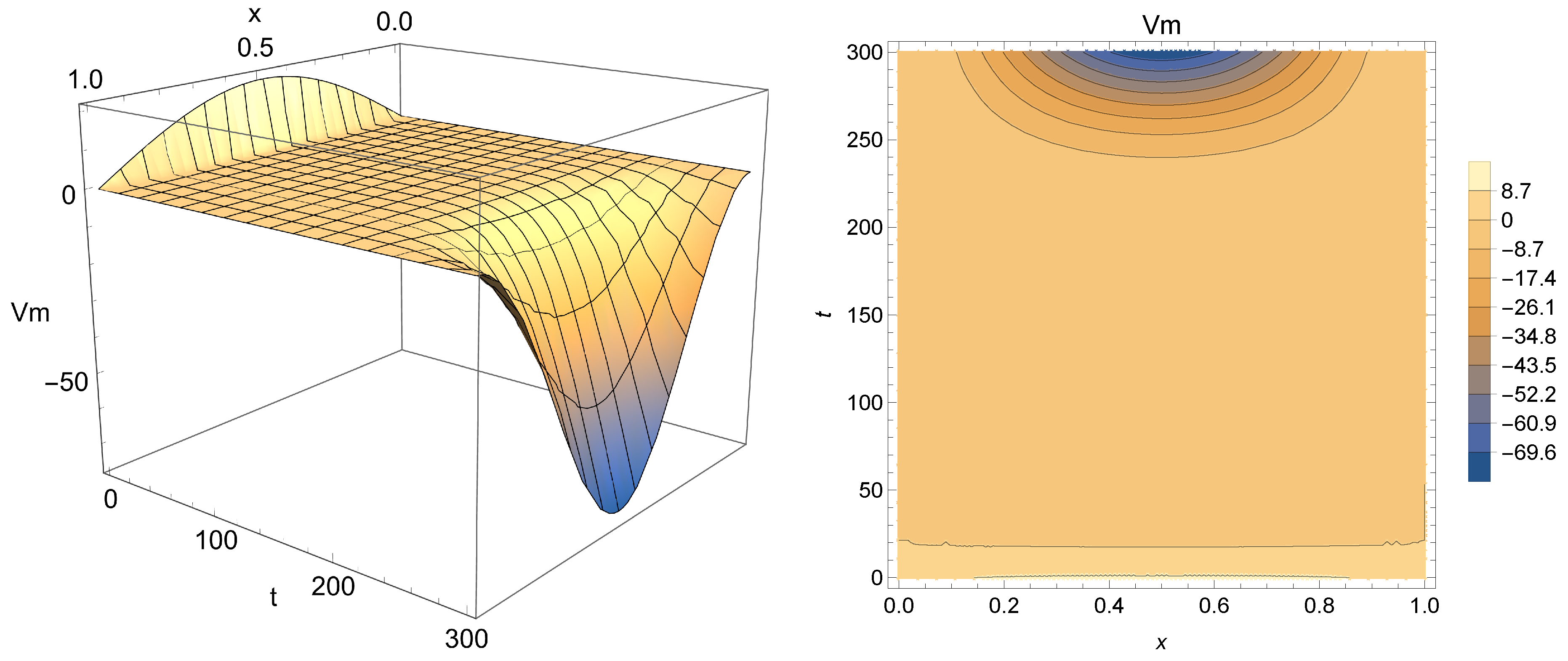
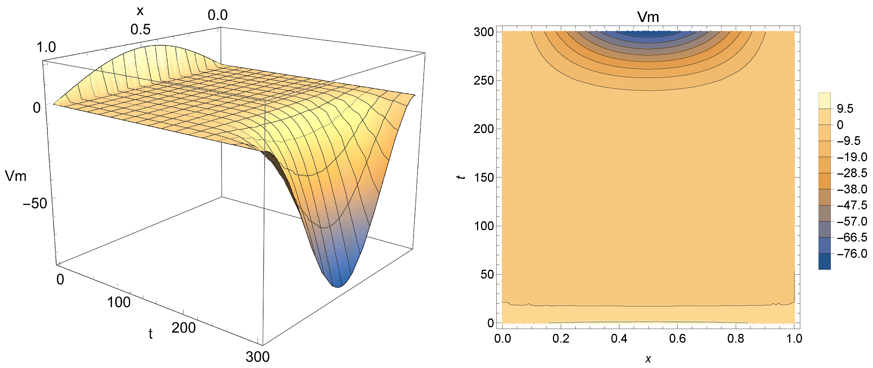
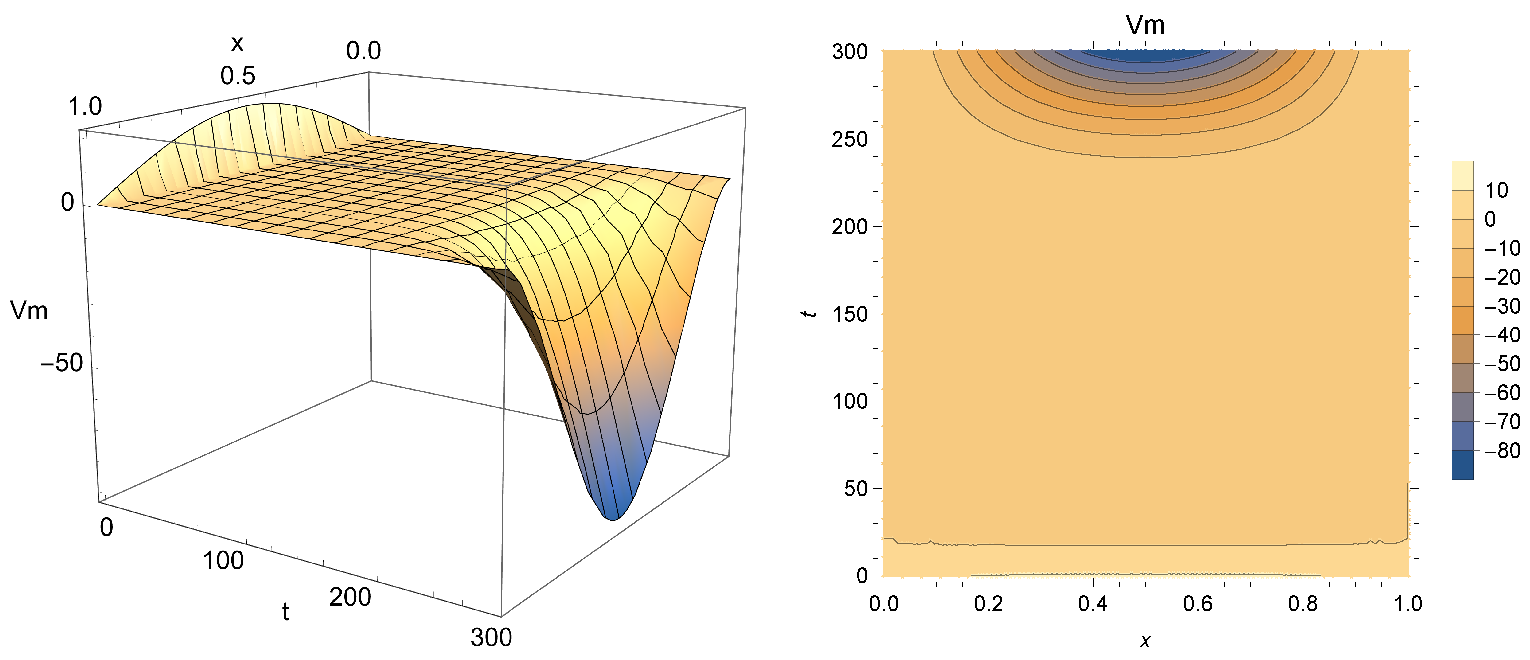
4.2. One-Dimensional Nonhomogeneous Case
The one-dimensional nonhomogeneous case can be simulated by using the same parameters from
Section 4.1 in Equation (
18). In this case,
must be considered to capture the dynamics between electric current and capacitance of the membrane tissue. Following from
Figure 1, one might use this scenario to represent Phases 2 and 3 of the membrane potential cycle, imposing
(which is negative by definition) to cause repolarization. This behavior considers the abrupt change during said phase of the action potential process, where there is a closure of calcium channels with an increasing exit of potassium from the myocyte cells, thus causing muscle contraction. Hence, in order to ensure continuity while still fulfilling that role,
is empirically defined as a sigmoidal function
In this context,
Figure 5,
Figure 6 and
Figure 7 present Equation (
18) for
(i.e., integer-order case),
and
, respectively.
From analyzing the results obtained, one can conclude that this solution may indeed be used for modeling Phases 2 and 3 of the membrane potential process, with smaller values of
acting as a smoothing factor in the dynamics of the electricity throughout cardiac tissue. Accordingly, models with
close to one provide a faster diffusion of electricity and, for that reason, the change in polarity caused by
is dismissed more quickly. Smaller values of
(in particular,
), on the other hand, enable the model to achieve a more significant drop, closer to the −90 mV mark, which is the actual value for the polarized state of the myocardium membrane [
55]. One can also see that for
ms,
will continue to drop, not stabilizing as the membrane potential after Phase 3, thus indicating that the nonhomogeneous solution should be used carefully to model the aforementioned phenomena.
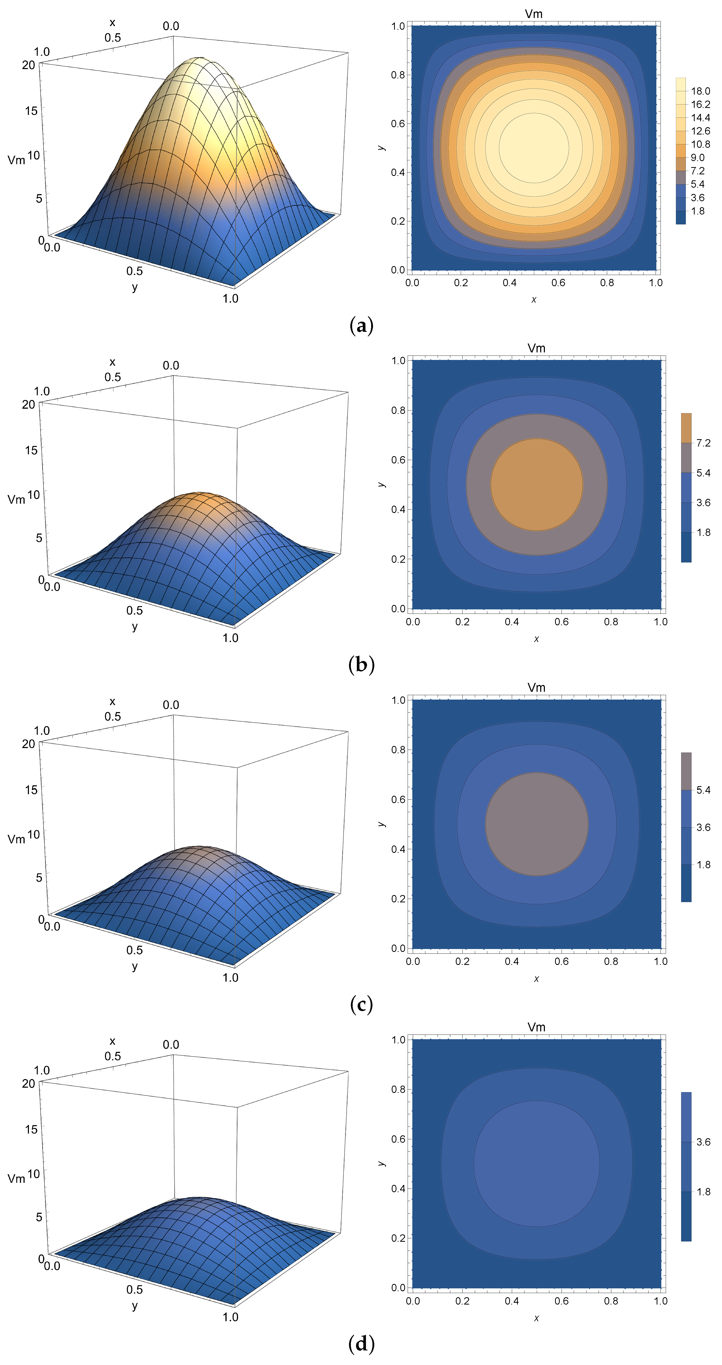
4.3. Two-Dimensional Homogeneous Case
The 2-D homogeneous solution given by Equation (
27) is analogous to the one expressed by Equation (
10) and numerically simulated in
Section 4.1 with an extended spatial variable
y. For that reason, it will be employed to virtualize only Phase 2 of the membrane potential process. The spatial domain is chosen as
mm and
mm. The initial condition is chosen as
mV to model the peak potential after polarization.
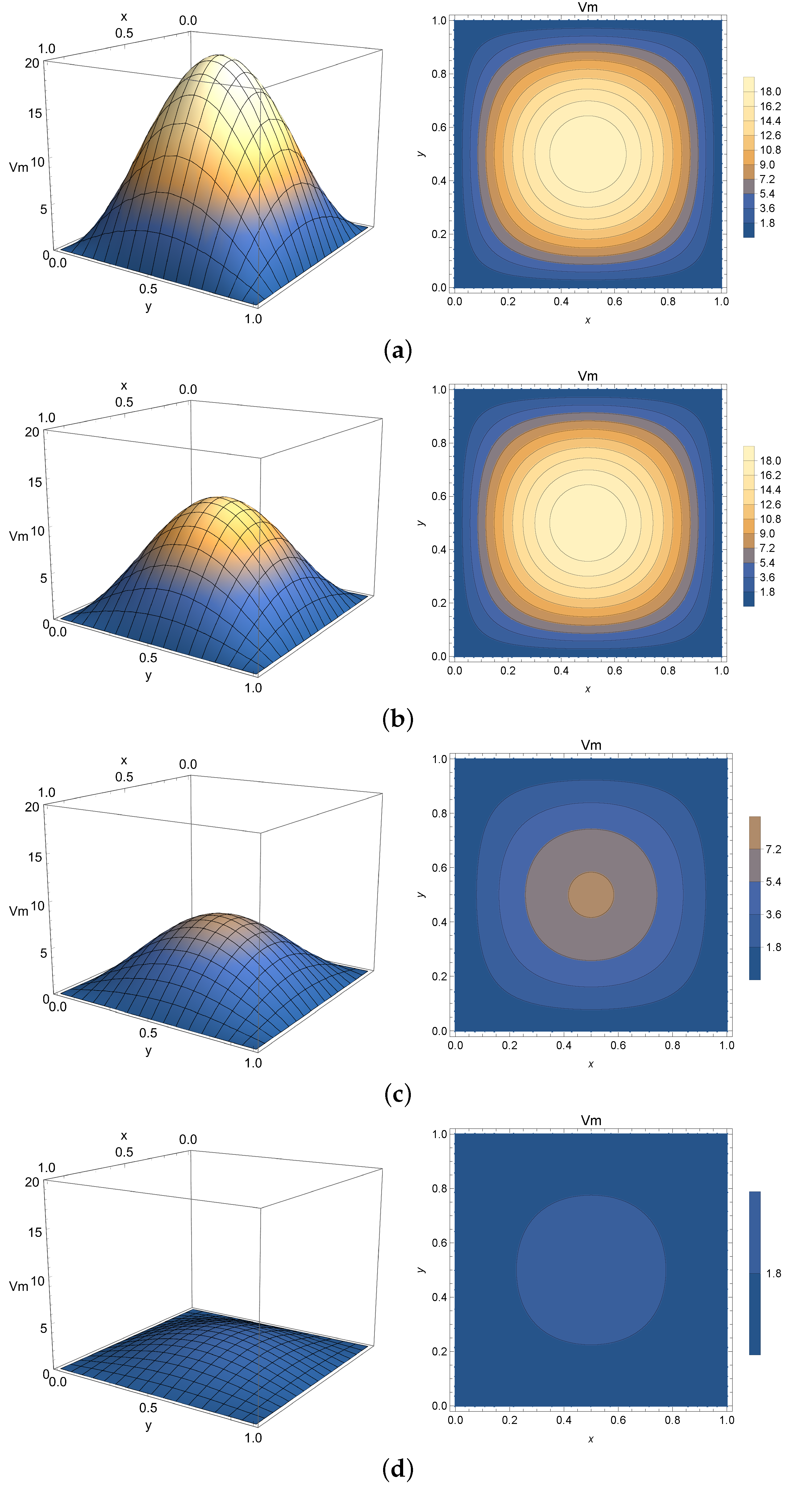
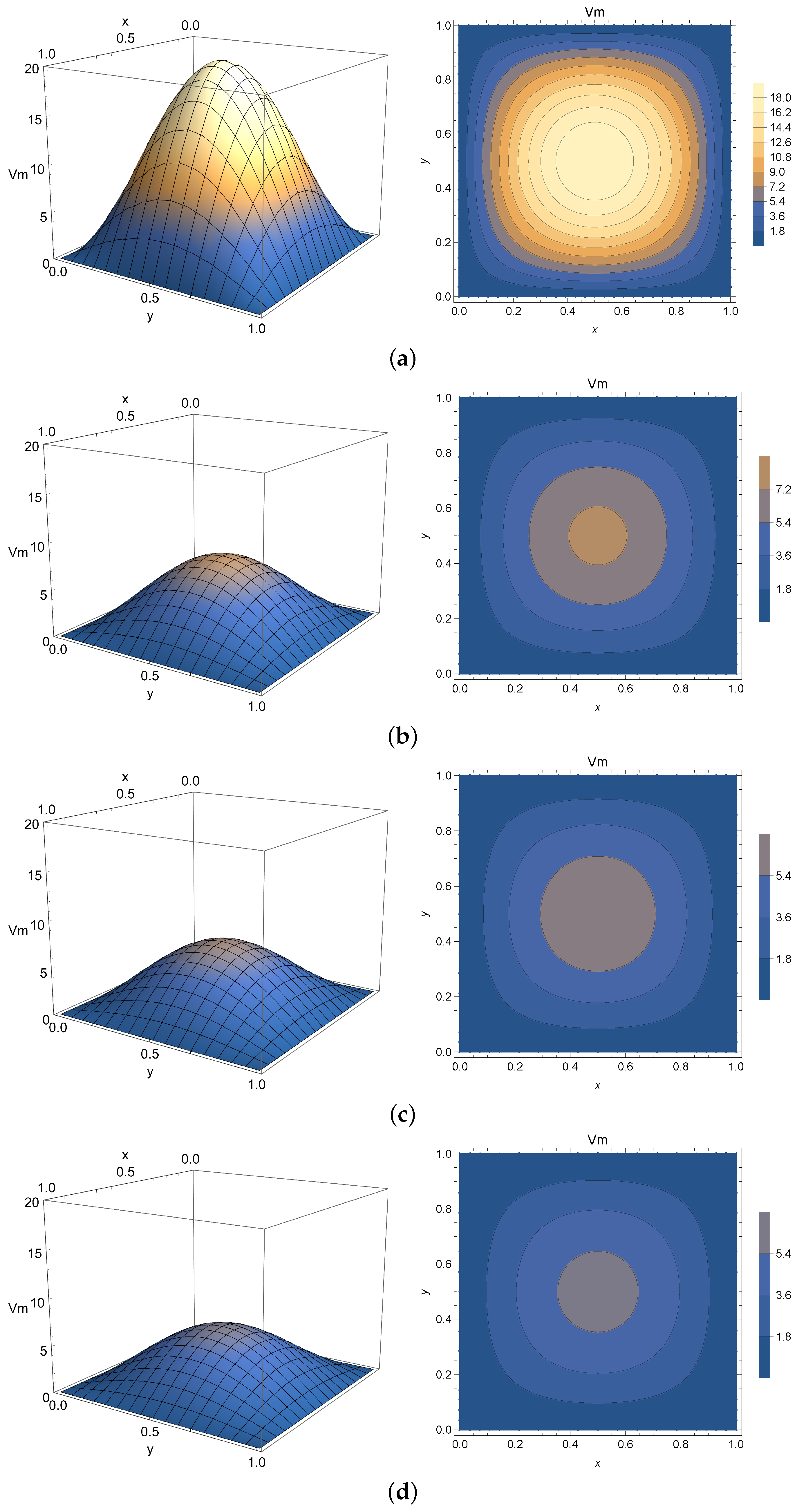
Once again,
Figure 8,
Figure 9 and
Figure 10 present the virtualized scenarios for
(integer-order case),
, and
. Each subfigure represents the system at a determined timestamp. In line with previous results, this model can be used to represent Phase 2 of the membrane potential, depicting the slight potential decrease right after the depolarization peak. One can see that in this case, the phenomenon occurs faster than expected. Accordingly, smaller values of
can impose a model where the diffusion of electricity throughout the tissue is slower, implying that this parameter can be used to fine-tune the model to describe a slower progression into the plateau phase if required.
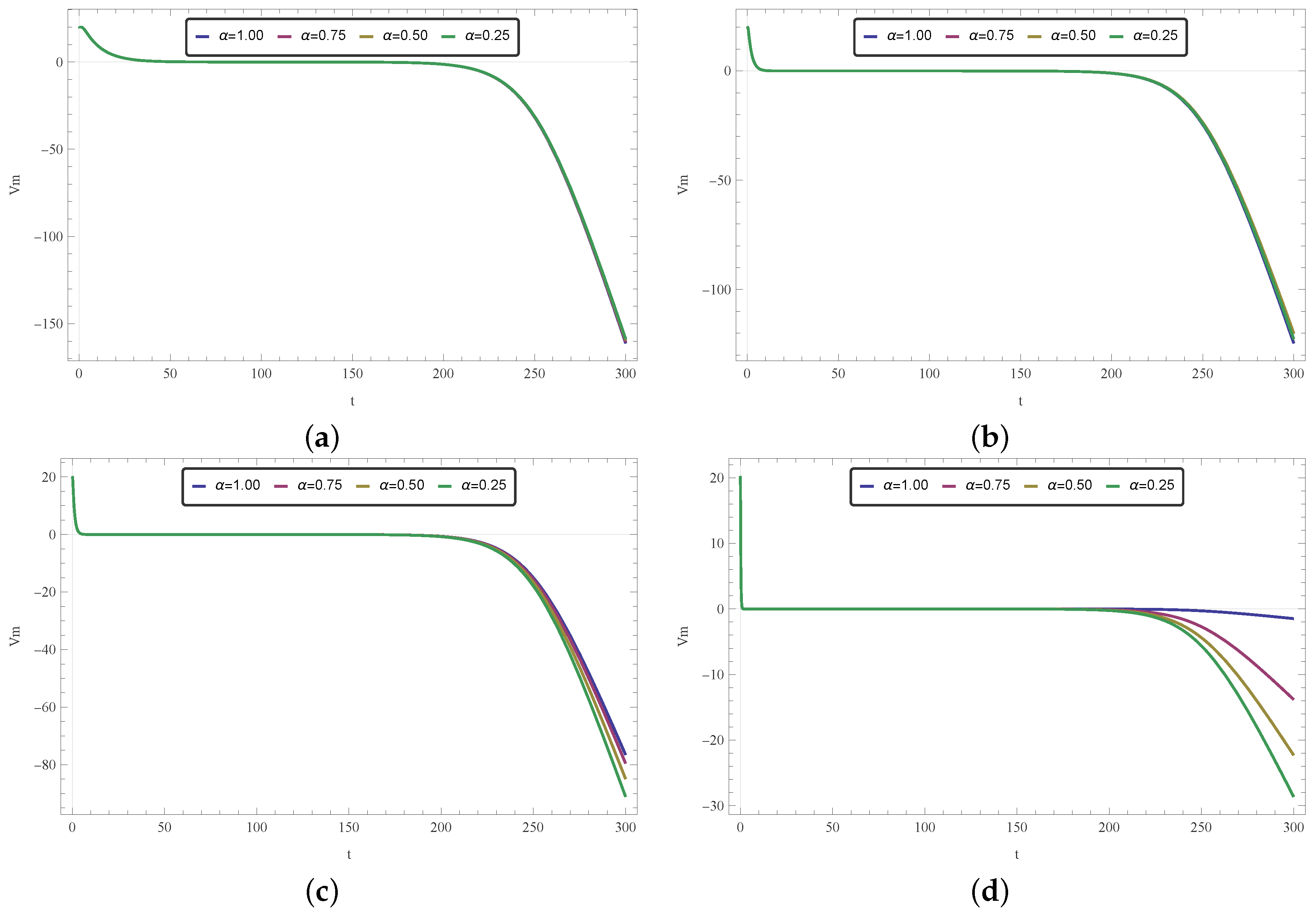
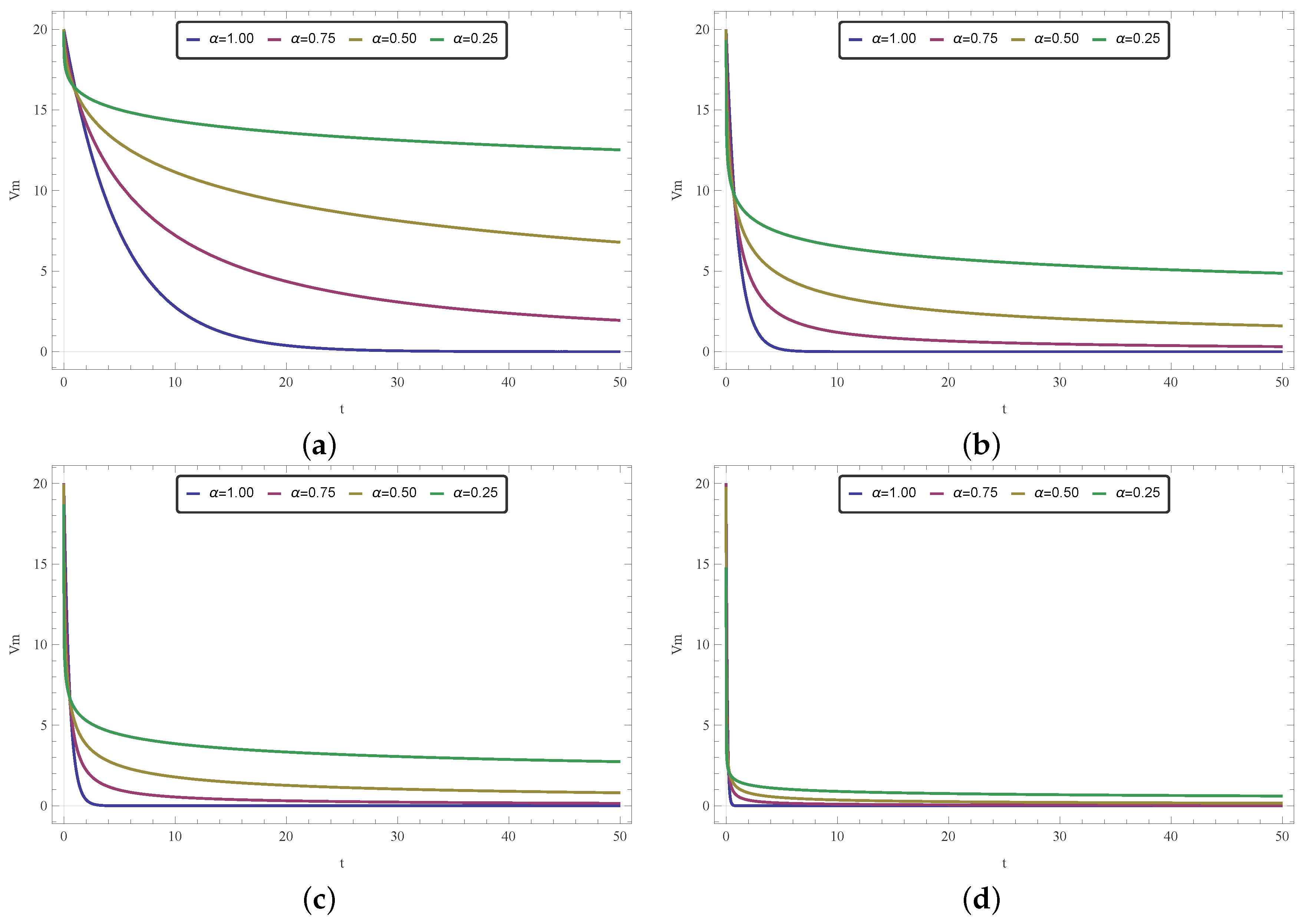
4.4. The Role of the Fractional Order and the Diffusivity Parameter k
Although both k and fractional order can be used at the modeler’s discretion to control the behavior of the model, thus adjusting it to fulfill a desired goal, they have very different roles. In this paper, we have opted to restrict the customizable aspect of the model exclusively to , as a means of focusing on the effects of a fractional time operator. Nevertheless, in order to further explore the model and succinctly discuss the differences between the effects of those two parameters, in this section we conduct some brief exploratory simulations on that matter.
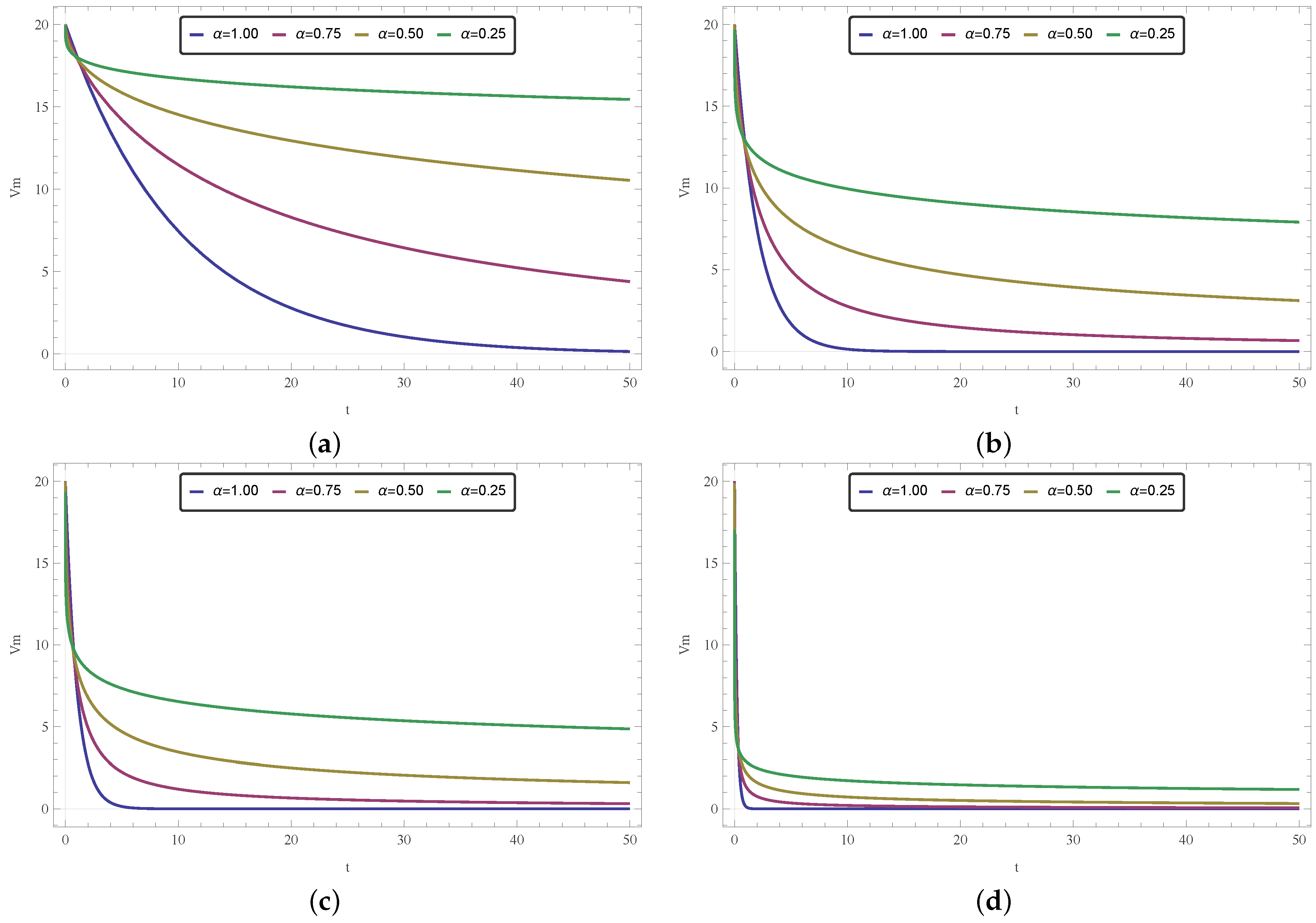
By neglecting the spatial aspect of the proposed model, we explore temporal curves for the 1-D homogeneous (
Figure 11), 1-D nonhomogeneous (
Figure 12), and 2-D homogeneous (
Figure 13) cases. The curves were obtained by employing Equations (
10) and (
18) with
, and Equation (
27) with
, for different values of
. As part of the exploratory approach, we repeated the simulations for different values of
k around the reference given in [
57].
By looking at the figures, one can see that the variation of
and
k affects the model quite differently. While
k is related to conduction velocity and how quickly a signal travels, the arbitrary (or fractional) order
regards how a signal (or information) lingers against time. This later effect concerns the memory effect, a feature present in fractional models. Even if these concepts seem similar, and effectively translate to how fast electricity diffuses through tissue, they are not the same and they do not yield the same results, as one can see in these temporal simulations. We believe that the curves shown in
Figure 11,
Figure 12 and
Figure 13 encourage the fractional approach even more since it suggests that different
values could allow the model to describe behaviors not possible by changing only
k (with the integer version of the model).
5. Final Remarks
In this paper, we investigate the dynamics of a class of fractional time-partial differential equations modeling the dynamics of some phases of the fast action potential in cardiac tissue. As main contributions, analytical solutions were derived and proposed for homogeneous and nonhomogeneous cases. Both one-dimensional and bidimensional spatial variations were considered. In the models, the time-fractional derivative order can be interpreted as a “tuning knob” to modulate how the processes are described, functioning as an additional parameter to improve the capabilities of the model to reproduce the aforementioned phenomena.
We conducted numerical simulations by employing the obtained solutions to model particular phase dynamics of the membrane action potential of the ventricular myocyte. Overall, the results indicate that the investigated equations can model the conduction of the action potential through the cardiac membrane, particularly regarding Phases 2 and 3 of the aforementioned impulse progression, with values below apparently enabling the model to achieve a better description of the typical −90 to 20 mV range of the process.
Accordingly, while there is not a fixed range or optimal order identified, overall fractional models with smaller values of seem to provide an extra tool to control the modeling dynamics of electrical impulses, with the potential of being used to describe attenuated electrical diffusion in the tissue or to represent other cardiac signal progressions. Simulations also highlight the differences and underlining physical distinctness of the effect on the model in comparison to other parameters such as diffusivity k.
While the results obtained here are encouraging, further studies should be conducted. Firstly, more information and data are needed to factually assess the performance of derived models, including experimental and clinical comparison or a benchmarking with other formal cardiac models. Secondly, by means of this comparison, one can try to identify which value is more suitable for each action potential phase, or even develop a variable that could, in theory, model the entire phenomenon. Last but not least, there is also the possibility of investigating the implementation of the model herein discussed as an additional tool in cardiac pacemaker and rhythm control models.


