Article

How Many Fractional Derivatives Are There?

1
IDMEC, Instituto Superior Técnico, Universidade de Lisboa, 1049-001 Lisboa, Portugal
2
Centre of Technology and Systems–UNINOVA and Department of Electrical Engineering, NOVA School of Science and Technology of NOVA University of Lisbon, Quinta da Torre, 2829-516 Caparica, Portugal
3
LAETA/INEGI, Faculty of Engineering, University of Porto, 4200-465 Porto, Portugal
*
Author to whom correspondence should be addressed.
Mathematics 2022, 10(5), 737; https://doi.org/10.3390/math10050737
Submission received: 24 January 2022 / Revised: 21 February 2022 / Accepted: 23 February 2022 / Published: 25 February 2022

Abstract

:
In this paper, we introduce a unified fractional derivative, defined by two parameters (order and asymmetry). From this, all the interesting derivatives can be obtained. We study the one-sided derivatives and show that most known derivatives are particular cases. We consider also some myths of Fractional Calculus and false fractional derivatives. The results are expected to contribute to limit the appearance of derivatives that differ from existing ones just because they are defined on distinct domains, and to prevent the ambiguous use of the concept of fractional derivative.

1. Introduction

Four centuries after the first reference to the possibility of non integer order derivatives, the presently termed Fractional Calculus (FC) has reached a crossroads where multiple definitions are mixed, causing a huge confusion that makes life very difficult for those who only intend to make applications in Science and Engineering. In fact, the first reference was found in a letter from Leibniz to J. Bernoulli [1]. Although Euler (1730), Fourier (1822), and Abel (1823) touched on the problem, the true father of FC was Liouville (1832) [2,3], in spite of their many difficulties to impose their vision, due to a main obstacle: At that time, the inverse Laplace integral was unknown. Therefore, Liouville could not find a simple way of expressing a function in terms of exponentials that were the basis for his findings. Anyway, the main definitions we find today are based on the formulæ presented by Liouville, mainly the Riemann–Liouville [4], (Dzherbashian)-Caputo [5,6], and Grünwald-Letnikov [4] definitions. However, and based on these derivatives, new ones have been proposed alongside these, such as Hadamard’s [6] or Marchaud’s [4]. Consequently, the number of currently existing fractional derivatives (FDs) is so high, which became the biggest obstacle to the diffusion of FC in Science and Engineering.
If we also consider the pseudo-derivatives and the disguised integer order derivatives, we conclude that the situation is really confused and confusing. Trying to introduce some order in the field, Oliveira and Machado, first, and Teodoro et al., more recently [7,8], listed such derivatives and introduced a classification according to some specified criteria. However, these papers included some operators that can hardly be classified as FDs. On the other hand, in recent years a great discussion took place in forums, conferences and articles, where there is a great confusion between the concepts of system and derivative. In a sequence of papers, Ortigueira and Machado tried to clarify the situation by proposing a coherent definition of FD [9], a description of FD suitable for applications in Science and Engineering [10], and introducing the FD in the context of fractional linear systems [11].
In this text, we make another step to clarify the situation, by introducing a step-down procedure. We recover the unified fractional derivative (UFD) obtained in [11] after a four step unification, and proceed as if this UFD were a mother derivative, defined by two parameters (order and dissymmetry), from which all the derivatives listed in [7,8] emerge as particular cases [12]. We will work in the context of Laplace and Fourier transforms. This includes most of the interesting functions and distributions used in practical applications.
We could go further by considering the tempered FDs [13,14], but we will not do so, in order to keep ourselves in the context of the derivatives introduced in [7,8]. On the other hand, we directed our attention to what we can call shift invariant derivatives, without considering the scale invariant ones such as the Hadamard [6] and the quantum [15] derivatives, as well as the discrete-time derivatives [16,17,18]. We will also not consider variable order derivatives [17]. Some operators, sometimes called FDs, are analyzed and put in the correct framework.
The paper is outlined as follows. In Section 2, we define fractional derivative. The UFD and its main properties is introduced in Section 3. The derivatives to referred in [7,8] are then obtained sequentially as particular cases through suitable choice of the parameters and working domain (Section 4). The other operators that, according to our framework, cannot be considered as FD will be treated in Section 5. Section 6 concludes the paper with a reflection on which definitions ought to be chosen.
Remark 1.
We adopt here the following assumptions:
  • We work on R .
  • We use the two-sided Laplace transform (LT):
    F ( s ) = L f ( t ) = R f ( t ) e s t d t ,
    where f ( t ) is any function defined on R and F ( s ) is its transform, provided that it has a non empty region of convergence (ROC).
  • The Fourier transform (FT), F f ( t ) , is obtained from the LT through the substitution s = i κ , with κ R .

2. What Is a Fractional Derivative?

In Signal Processing, independently of the applications to Electrical, Mechanical, Biomedical or any other Engineering field, there is a very simple way of defining a FD: a FD is a linear operator described by Bode diagrams that are straight lines [11]. In terms of the FT we can write
F D θ γ f ( t ) = | ω | γ e i θ π 2 sgn ( ω ) F f ( t ) t , ω R ,
where γ , θ R , and D θ γ represents the derivative. The operator
Ψ θ γ ( ω ) = | ω | γ e i θ π 2 sgn ( ω ) ω R
is the frequency response of the derivative. Functions A ( ω ) (amplitude) and ϕ ( ω ) (phase), when represented in a logscale for ω > 0 , are expressed by straight lines. These can be used to define a FD.
However, we need a criterion independent of any transform. As in [9], we define as FD an operator that verifies the following (wide sense) criterion.
Definition 1.
An operator is considered a FD in wide sense if it enjoys properties P defined as:
P1 
Linearity
The operator is linear.
P2 
Identity
The zero order derivative of a function returns the function itself.
P3 
Backward compatibility
When the order is integer, FD gives the same result as the ordinary derivative.
P4 
The index law
D α D β f ( t ) = D α + β f ( t )
holds for α < 0 and β < 0 .
P5 
The generalized Leibniz rule
D α f ( t ) g ( t ) = i = 0 α i D i f ( t ) D α i g ( t )
holds. As is clear, when α = N Z + , we obtain the classical Leibniz rule.
The index law property can be modified to include positive orders. This leads to the strict sense criterion. This criterion has the same five conditions, but P4 is modified to:
P’4
The generalized index law
D α D β f ( t ) = D α + β f ( t )
holds for any α and β .
This is very important because it allows the existence of the inverse derivative: the anti-derivative. It is convenient to state the differences between anti-derivative and “primitive”:
  • The anti-derivative is unique.
  • The anti-derivative is a left and right inverse, while any primitive is only right inverse.
These criteria allow us to clarify the situation of some “disguised” order one derivatives and put out some frauds.

3. Unified Fractional Derivative

In [11], a UFD incorporating most of the useful derivatives was presented and its properties studied. It is described as follows.
Definition 2.
Let f ( t ) be a function defined on R ( C ), and let α > 1 if θ ± α , or α R if θ = ± α . We define a UFD of GL type by
D θ α f ( t ) : = lim h 0 + h α n = + ( 1 ) n Γ α + 1 Γ α + θ 2 n + 1 Γ α θ 2 + n + 1 f ( t n h ) ,
where α is the derivative order and θ the asymmetry parameter. We define also a general integral formulation for the unified anti-derivative through
D θ α f ( t ) = 1 sin α π Γ ( α ) R f ( t τ ) sin α + θ · sgn ( τ ) π 2 | τ | α 1 d τ ,
where sgn ( . ) denotes the signum function.
The integral in (8) can be regularized in order to become valid for positive orders [12]. This is done with the substitution
f ( t τ ) f ( t τ ) 0 N 1 ( 1 ) m f ( m ) ( t ) m ! τ m ,
with N = γ + 1 .
Some known properties of this derivative can be drawn [12,15]. The main ones are:
  • Fourier transformation
    It was introduced above in (2). It permits obtaining (8) from (7), using the convolution theorem. It has another consequence:
    D θ α f ( t ) = cos θ π 2 D 0 α f ( t ) + sin θ π 2 D 1 α f ( t ) .
  • Eigenfunctions
    Let f ( x ) = e i κ x , κ , x R . Then,
    D θ β e i κ x = κ β e i π 2 θ · sgn ( κ ) e i κ x ,
    meaning that the sisoids are the eigenfunctions of the UFD with eigenvalue Ψ θ β ( κ ) = κ β e i π 2 θ · sgn ( κ ) .
  • Periodicity in θ
    The UFD is periodic in θ with period 4
    D θ β f ( x ) = ( 1 ) n D θ + 2 n β f ( x ) , n Z ,
    as we observe from (2).
  • Additivity and commutativity of the orders
    D θ 1 β 1 D θ 2 β 2 f ( x ) = D θ 1 + θ 2 β 1 + β 2 f ( x ) .
    In particular, conjugating (13) with (12),
    D 0 β 1 D 0 β 2 f ( x ) = D 0 β 1 + β 2 f ( x ) ,
    D 1 β 1 D 1 β 2 f ( x ) = D 0 β 1 + β 2 f ( x ) ,
    D 0 β 1 D 1 β 2 f ( x ) = D 1 β 1 + β 2 f ( x ) ,
    D β 1 β 1 D β 2 β 2 f ( x ) = D β 1 + β 2 β 1 + β 2 f ( x ) ,
    D θ β 2 D θ β 2 f ( x ) = D 0 β f ( x ) ,
    D θ β 2 D 1 θ β 2 f ( x ) = D 1 β f ( x ) .
  • Existence of inverse derivative
    From (13), the anti-derivative exists when β 2 = β 1 and θ 1 = θ 2 . Therefore,
    D θ β D θ β f ( x ) = D θ β D θ β f ( x ) = f ( x ) .
  • Identity operator
    According to (13) and (20), the identity operator is defined by
    D 0 0 f ( x ) = f ( x ) .
Suitable choices of these parameters allow us to recover the causal, anti-causal, and bilateral (acausal) derivatives. The particular, most interesting, cases are obtained from (7) and (8). In terms of the frequency response, we have
  • forward derivative, θ = α
    Ψ α α ( ω ) = | ω | α e i α π 2 sgn ( ω ) = ( i ω ) α
  • backward derivative, θ = α
    Ψ α α ( ω ) = | ω | α e i α π 2 sgn ( ω ) = ( i ω ) α
  • Riesz derivative and potential, θ = 0
    Ψ 0 α ( ω ) = | ω | α
  • Feller derivative and potential, θ = 1
    Ψ 1 α ( ω ) = i | ω | α sgn ( ω )
  • Hilbert transform, α = 0 , θ = 1
    Ψ 1 0 ( ω ) = e i π 2 sgn ( ω ) = i sgn ( ω ) .
From these expressions and using (7) it is possible to devise numerous derivatives by:
  • choosing particular values of the parameters α and θ ,
  • restricting the domain of the function at hand.

4. One-Sided Derivatives

4.1. The GL Derivatives

The great importance of one-sided derivatives in applications leads us to study them in detail. Taking (7) with γ = α and θ = ± α we obtain the forward (left) and backward (right) GL derivatives that with some manipulation can be written as
D ± α f ( t ) : = lim h 0 + h α n = 0 + α n n ! f ( t n h ) .
As it is easy to verify, the forward derivative + is causal, while the backward − is anti-causal. This kind of derivatives was proposed first by Liouville [2].
For functions with LT (or FT), we can write
L D θ α f ( t ) = ( ± s ) α F ( s ) , ± ( s ) 0 ,
where F ( s ) = L f ( t ) . As is known from the study of the LT, the LT of a right (left) function, f ( t ) = 0 , t < a ( t > a ) , a R has a ROC defined by ( s ) > 0 ( ( s ) < 0 ). If f ( t ) is absolutely of square integrable, then it has FT and we can write
Ψ ± α ( s ) = ( ± s ) α , ± ( s ) 0 .
Function Ψ ± α ( s ) = ( ± s ) α with suitable ROC is the transfer function (TF) of the derivative (also called differintegrator).

4.2. The Impulse Response

The relations (28) and (29) suggest the existence of two operators that, convolved with suitable functions, give their FDs. For α > 0 the LT inverse of s α does not exist as regular function. However, it has a generalized inverse represented by the pseudo-function
ψ ± α ( t ) = ± t α 1 Γ ( α ) u ( ± t ) ,
where + (−) corresponds to the causal (anti-causal) case. The pseudo-function (30) is called impulse response (IR) of the differintegrator. The use of the convolution resulting from (28) would allow us to obtain the derivative D ± α f ( t ) . For α < 0 , there is no particular difficulty and we obtain from (8)
D ± α f ( t ) = 1 Γ ( α ) 0 f ( t τ ) τ α 1 d τ .
The expression corresponding to the anti-causal case was proposed almost with the above form by Liouville [3]. The causal case was deduced from the anti-causal by Serret [1,19]. Liouville’s formula included a factor ( ± 1 ) α to ensure that
L D ± α f ( t ) = s α F ( s )
for both expressions, although the ROC will be defined by ± R e ( s ) > 0 . In most texts, such factor is removed. In time problems it must be kept, but, in space applications, it plays no relevant role. Therefore, we will omit it in the following. The finite domain versions of (31) are called RL integrals:
D a + α f ( t ) = 1 Γ ( α ) a + t f ( t τ ) τ α 1 d τ
and
D b α f ( t ) = 1 Γ ( α ) t b f ( t τ ) τ α 1 d τ .
We will assume these forms in the following.

4.3. Liouville’s Derivatives

Liouville [2] noted that (31) becomes singular when the order is positive (i.e., when it corresponds to a derivative). This problem can be solved with the regularization [15,17]
D f α f ( t ) = 1 Γ ( α ) 0 τ α 1 f ( t τ ) 0 N 1 ( ) m f ( m ) ( t ) m ! τ m d τ ,
that we will call regularized Liouville (L) derivative. The first regularization of the Liouville integral (31) was done by Marchaud [4]. However, their regularization only verifies the derivative property of the LT if the order is less than 1.
Instead of a regularization, Liouville devised a trick for solving the singularity problem that we can describe as
s α = s N s α N = s α N s N ,
where N > 0 verifies N > α . The most usual choice is N = α . Basically, it consists of transferring the singular behavior to an integer order derivative. The first approach leads to the so-called Liouville derivatives [4],
D + α f ( t ) = 1 Γ ( N α ) d N d t N 0 f ( t τ ) τ N α 1 d τ
and
D α f ( t ) = ( 1 ) N Γ ( N α ) d N d t N 0 f ( t + τ ) τ N α 1 d τ ,
that can be rewritten as
D + α f ( t ) = 1 Γ ( N α ) d N d t N t f ( τ ) ( t τ ) N α 1 d τ
and
D α f ( t ) = ( 1 ) N Γ ( N α ) d N d t N t f ( τ ) ( t τ ) N α 1 d τ .
This one is sometimes called “Weyl derivative” [8].
Liouville’s second procedure leads to what can be called Liouville–Caputo (LC) derivatives [20]:
D + α f ( t ) = 1 Γ ( N α ) t f ( N ) ( τ ) ( t τ ) N α 1 d τ
and
D α f ( t ) = ( 1 ) N Γ ( N α ) t f ( N ) ( τ ) ( t τ ) N α 1 d τ .
Remark 2.
We must remark that:
1.
These derivative definitions are equivalent for functions with LT or FT.
2.
For some particular classes of functions this may not be correct, e.g., the L derivatives are better than the LC. Possible causes for this are:
  • The convolution makes the functions smoother;
  • The derivative may introduce roughness or spikes.
3.
These 2 + 2 formulations lead to most derivatives described in [7,8]. We must reinforce something very important: all the above defined derivatives are valid for functions defined in any interval of R . This means that we do not need to change the definitions to accommodate them to the domain of the function at hand. One thing is the definition, another one is the computation of the derivative. It is a situation similar to the one we find in the LT or FT. We do not need to change the definitions to agree with the domain of the function. Therefore, most derivative definitions in [7,8] have no reason to be considered as autonomous derivatives.
4.
These derivatives do not introduce any initial conditions.
5.
For a given derivative, there is always an anti-derivative.
These derivative formulations using (28) and the convolution are related as Figure 1 illustrates, and collected in Table 1, where
a b = Γ ( a + 1 ) Γ ( b + 1 ) Γ ( a b + 1 ) , if a , b , a b Z ( 1 ) b Γ ( b a ) Γ ( b + 1 ) Γ ( a ) , if a Z b Z 0 + 0 , if [ ( b Z b a N ) a Z ] ( a , b Z | a | > | b | )

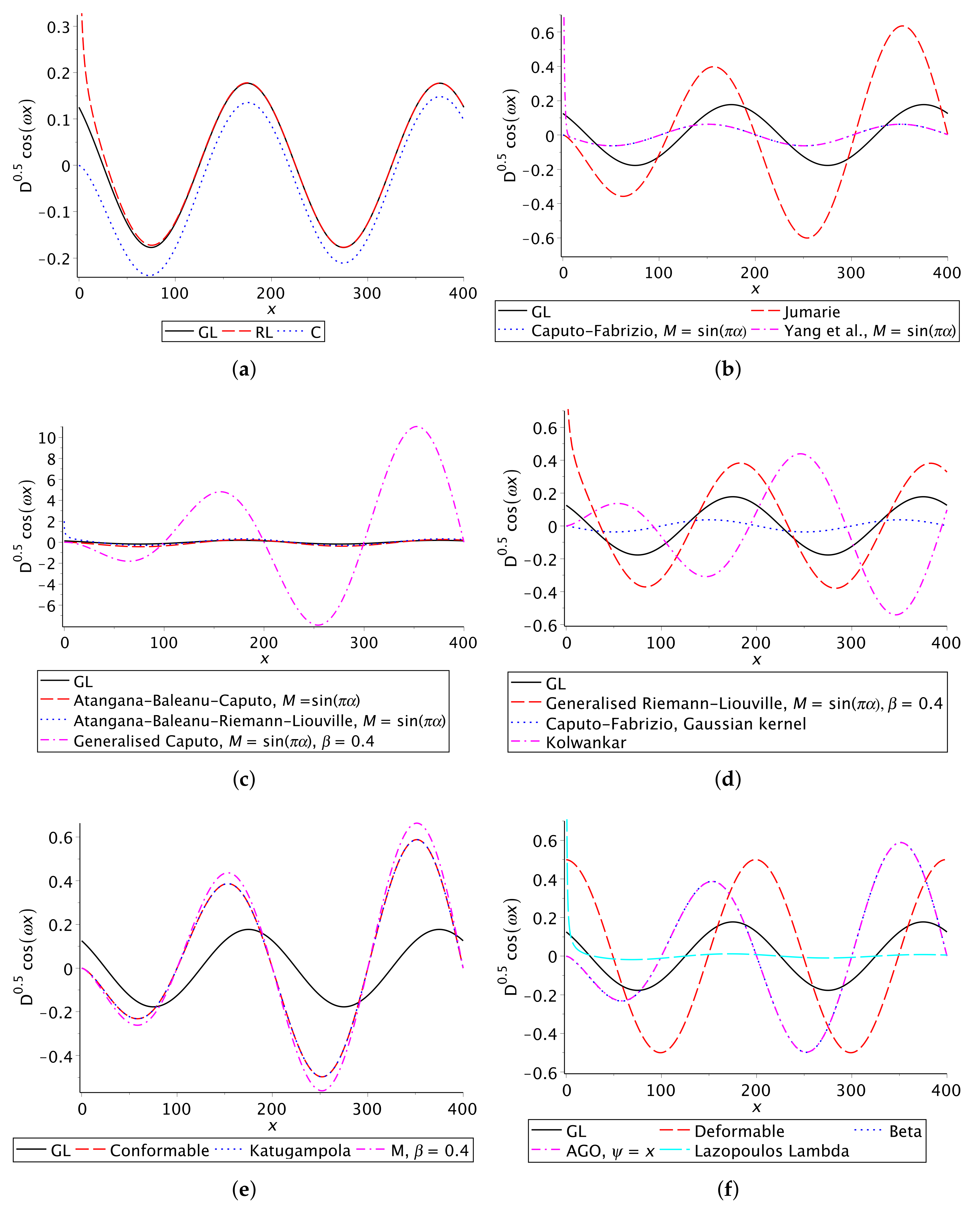
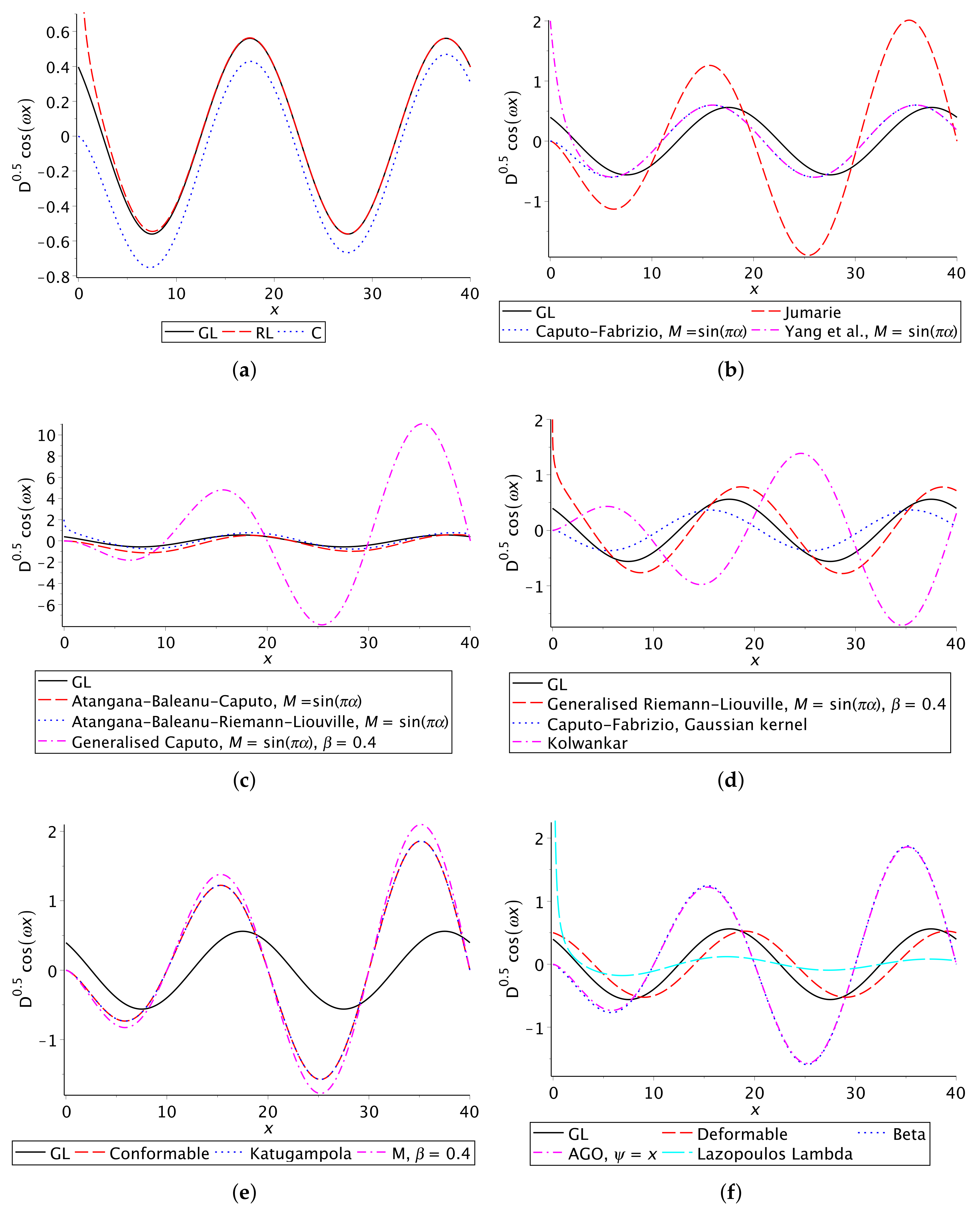
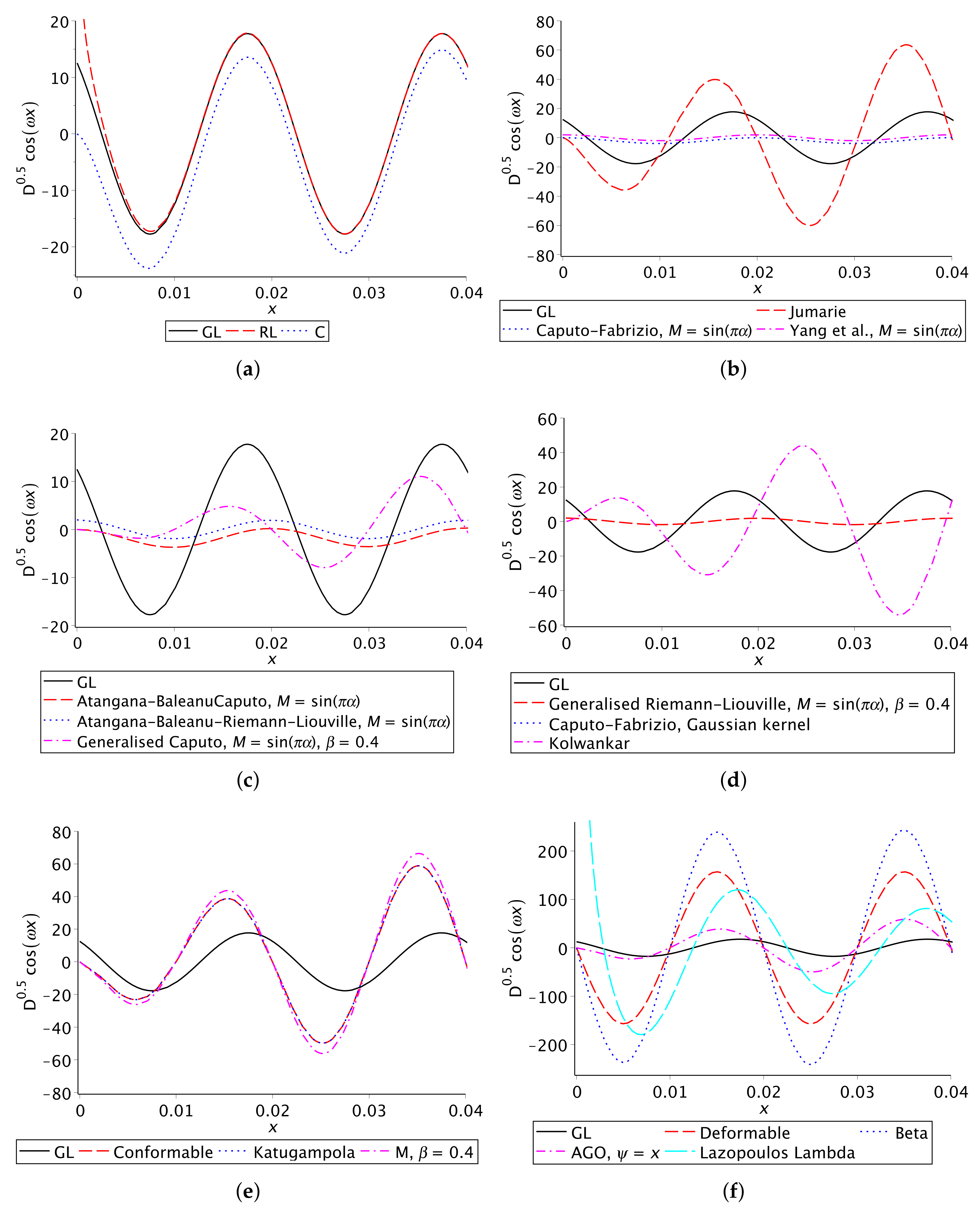
4.4. RL and C Derivatives

Despite the high degree of generality exhibited by the above derivatives, they are not used in most papers. In fact, such papers use derivatives specialized for functions that are defined on intervals [ a , b ] , < a < b < [4,6]. Usually a 0 so that right functions are assumed. When a = 0 we use frequently the designation “causal function”. The GL derivatives assume the form
GL D a + α [ f ( x ) ] = lim h 0 1 h α k = 0 n ( 1 ) k Γ ( α + 1 ) f ( x k h ) Γ ( k + 1 ) Γ ( α k + 1 ) , n h = x a
and
GL D b α [ f ( x ) ] = lim h 0 1 h α k = 0 n ( 1 ) k Γ ( α + 1 ) f ( x + k h ) Γ ( k + 1 ) Γ ( α k + 1 ) , n h = b x .
This was the procedure of Grünwald [21] and Letnikov [22]. Therefore, they are nothing else than the application of (27) to bounded support functions and so they are not new derivatives. For the integral formulations, the contributions of Liouville and Riemann [23] were joined to obtain the Riemann–Liouville (RL) derivative [4,6]; likewise, from the Liouville–Caputo derivative, the (Dzherbashian-)Caputo (C) derivative [5,6] is obtained. We have:
  • Riemann–Liouville (RL) derivatives
    R L D a + α f ( t ) = 1 Γ ( N α ) d N d t N a t f ( τ ) ( t τ ) N α 1 d τ , t > a
    and
    R L D b α f ( t ) = ( 1 ) N Γ ( N α ) d N d t N t b f ( τ ) ( t τ ) N α 1 d τ , t > a .
  • (Dzherbashian-)Caputo (C) derivatives
    C D a + α f ( t ) = 1 Γ ( N α ) a t f ( N ) ( τ ) ( t τ ) N α 1 d τ , t > a
    and
    C D b α f ( t ) = ( 1 ) N Γ ( N α ) t b f ( N ) ( τ ) ( t τ ) N α 1 d τ , t < b .
These formulations, collected in Table 2, are the ones most used, although they have several inconveniences, mainly the initial conditions problem they introduce [17]. However, they form the basis for many applications.

4.5. Multistep Derivatives

The procedure introduced in (36) can be generalized. For example,
s α = s N k s α N s k , α R + , N Z 0 + ,
with k < N and N > α . Then,
D α f ( t ) = D N k 1 Γ ( N α ) a t f ( k ) ( τ ) ( t τ ) N α 1 d τ .
This procedure was proposed by Davidson and Essex [8]. However, the derivative they proposed is valid only for functions which are null for t < 0 . Cavanati [8] introduced an algorithm that is a particular case obtained with k = N 1 .
Another similar algorithm was presented by Hilfer [24], also for causal functions. It can be stated as
s α = s μ ( 1 α ) s s ( 1 μ ) ( 1 α ) ,
where 0 < α , μ < 1 . It reads
D α f ( t ) = D μ ( 1 α ) 1 Γ ( 1 μ ) ( 1 α ) d d x a t f ( τ ) ( t τ ) ( 1 μ ) ( 1 α ) d τ .
This approach can be generalized. For example, if 1 < α < 2 , then we can set
s α = s μ ( 2 α ) s 2 s ( 1 μ ) ( 2 α )
or
s α = s s μ ( 2 α ) s s ( 1 μ ) ( 2 α ) .
This kind of reasoning shows that, following this method, we can invent billions of “derivatives”. However, it is not clear how this is interesting in real life applications. Indeed, we are not introducing a new derivative, but using repeatedly one basic derivative. Some of the such derivatives were proposed because they introduced more favorable initial conditions. However, this is in general incorrect, since the initial conditions do not depend on the derivatives, but on the physical structure of the system at hand [17,25].

4.6. Second Generation Operators

The derivatives we introduced above are “shift invariant”. However, there are other derivatives that do not enjoy such properties, and therefore cannot be obtained from the UFD introduced above. It is the case of the Hadamard derivatives [6] that are “scale invariant”. Other examples are the “quantum derivatives” [15]. It is important to refer also the Marchaud derivatives [4] that exhibit a kind of regularization. On the other hand, some modifications and variable changes can be made in the above derivatives, leading to interesting operators that may not necessarily be considered to be derivatives when seen in the light of the above criterion [7,8]. They are introduced in Table 3.

5. Pseudo-Fractional-Derivatives

5.1. Some Comments

In many quarters, the treatment of FDs and systems was taken to be a quite difficult task. Therefore, simplified versions thereof were welcomed, even if some important features that characterize most systems were lost in the process — for example, in modeling natural or human-made systems that are essentially low-pass or bandpass systems. However, some proposed systems are high-pass, and then have limited usefulness; in the following, we describe some of them. We must remark that sometimes the word “fractional” is used as a “trade mark” that helps to “sell a product”. It is the case of the “Memory-dependent derivative” [26], that is nothing else than a running average.

5.2. “Derivatives” That Are High-Pass Filters

Consider a simple differential equation:
a 1 y ( t ) + a 0 y ( t ) = b 1 x ( t ) .
This equation is recognized easily as the model of the classic high-pass filter [27]. Its transfer function is
H ( s ) = b 1 s a 1 s + a 0 = b 1 a 1 s s + σ , ( s ) > σ = a 0 / a 1 .
One way of relating the input and output is:
y ( t ) = b 1 a 1 0 t e σ ( t τ ) x ( τ ) d τ .
This expression was chosen with this form to remember the Caputo derivative (41). Now set:
a 0 = α , a 1 = 1 α , b 1 = M ( α ) , σ = α 1 α
to obtain
y ( t ) = M ( α ) 1 α 0 t e α 1 α ( t τ ) x ( τ ) d τ .
This is the expression of the “famous” fractional Caputo-Fabrizio “derivative”. As is clear, it is neither a derivative, nor fractional.
Let us continue and substitute the exponential in (60) by the Mittag–Leffler function. We obtain also a fractional high-pass filter with TF given by
H ( s ) = M ( α ) 1 α s α s α + σ , ( s ) > 0 ,
that is called Atangana-Baleanu “derivative”. Attending to its FT, it is a system, but not a derivative. There are many variations of this operator, but they remain high-pass filters, not derivatives [8].
For a list of these and similar operators, see Table 4.

5.3. “Disguised” Order 1 Derivatives

The “local fractional derivative” introduced by Kolwankar reads [28]
D α f ( t ) = lim τ t D t α f ( τ ) f ( t ) ,
where D t α is the RL derivative. V. Tarasov [29] showed that, if α < 1 , this derivative is equivalent to the order 1 derivative, therefore not fractional.
A similar result can be found for the “conformable” derivative [30]
D α f ( t ) = lim ε 0 f t + ε t 1 α f ( t ) ε
and
D α f ( t ) = lim ε 0 f t e ε t α f ( t ) ε .
For differentiable functions and for both derivatives, this results in
D α f ( t ) = t 1 α d f d t ( t ) .
Several modified versions of these derivatives were proposed [8].
The so-called “fractal derivative” was introduced in [31] and reads
f ( t ) t α = lim s t f ( t ) f ( s ) t α s α .
It is a strange derivative that gives for differentiable functions, unless α = 1 .
For a list of these and similar operators, see Table 5.
Figure 2, Figure 3 and Figure 4 illustrate the results obtained with different FD formulations, when applied to compute the α = 0.5 order derivative of the function f ( x ) = cos ( ω x ) , for ω = { 0.01 π , 0.1 π , 100 π } , respectively. The derivatives are compared with the one obtained with the GL operator, which serves as baseline. In all cases we adopt a = 0 , while FD specific parameters are as presented in the legends of the graphs. We verify that some formulations fail to compute the derivatives accurately, while others diverge.
As is well known, the classic order 1 derivative of a sinusoidal is the same sinusoidal multiplied by the angular frequency and with a change of phase equal to π / 2 . Therefore, we expect something similar in the fractional case, at least after passing some time corresponding to the transient regime. This happens with those operators that we classified as derivatives. For the others, we have amplifications/attenuations and, in some cases, modulations, confirming that they are systems (filters), but not derivatives. Some have a non-acceptable behavior: they are unstable.

6. Which Derivatives?

After this journey into the world of FDs, it is important to answer the question: “Do we need such different formulations?”
In previous papers [10,11,12], some answers to this question were given.
  • In problems involving time, we have almost always to use causal derivatives. Therefore, the GL or one of the integral versions (37), (39), or (41) should be used.
  • In space problems, we can use the above formulæor the corresponding right-side versions, if there is any privileged direction. If this does not happen, we must use a two-sided derivative, preferably (2).
However, most derivatives described in [7,8] are particular cases, and the particularity is introduced by the domain. Therefore, do we need to define a new derivative each time the domain changes? This creates a big difficulty: we cannot keep increasing the number of derivatives, differing only because they are defined on different domains, which constrains the application fields.

Author Contributions

Conceptualization, M.D.O.; methodology, M.D.O.; formal analysis, all authors; writing—original draft preparation, all authors; writing—review and editing, all authors; visualization, A.M.L. All authors have read and agreed to the published version of the manuscript.

Funding

This work was partially funded by National Funds through the FCT-Foundation for Science and Technology within the scope of the CTS Research Unit—Center of Technology and Systems/UNINOVA/FC /NOVA, under the reference UIDB/00066/2020, and also by FCT through IDMEC, under LAETA, project UID/EMS/50022/2020.

Conflicts of Interest

The authors declare no conflict of interest.

References

  1. Dugowson, S. Les Différentielles Métaphysiques (Histoire et Philosophie de la Généralisation de l’ordre de Dérivation). Ph.D. Thesis, Université Paris Nord, Paris, France, 1994. [Google Scholar]
  2. Liouville, J. Memóire sur le calcul des différentielles à indices quelconques. J. L’École Polytech. Paris 1832, 13, 71–162. [Google Scholar]
  3. Liouville, J. Memóire sur quelques questions de Géométrie et de Méchanique, et sur un nouveau genre de calcul pour résoudre ces questions. J. L’École Polytech. Paris 1832, 13, 1–69. [Google Scholar]
  4. Samko, S.G.; Kilbas, A.A.; Marichev, O.I. Fractional Integrals and Derivatives; Gordon and Breach: Yverdon, Switzerland, 1993. [Google Scholar]
  5. Podlubny, I. Fractional Differential Equations: An Introduction to Fractional Derivatives, Fractional Differential Equations, to Methods of Their Solution and Some of Their Applications; Academic Press: San Diego, CA, USA, 1999; pp. 1–3. [Google Scholar]
  6. Kilbas, A.A.; Srivastava, H.M.; Trujillo, J.J. Theory and Applications of Fractional Differential Equations; Elsevier: Amsterdam, The Netherlands, 2006. [Google Scholar]
  7. De Oliveira, E.C.; Tenreiro Machado, J.A. A review of definitions for fractional derivatives and integral. Math. Probl. Eng. 2014, 2014, 238459. [Google Scholar] [CrossRef] [Green Version]
  8. Teodoro, G.S.; Machado, J.T.; De Oliveira, E.C. A review of definitions of fractional derivatives and other operators. J. Comput. Phys. 2019, 388, 195–208. [Google Scholar] [CrossRef]
  9. Ortigueira, M.D.; Machado, J.T. What is a fractional derivative? J. Comput. Phys. 2015, 293, 4–13. [Google Scholar] [CrossRef]
  10. Ortigueira, M.D.; Machado, J.A.T. Which Derivative? Fractal Fract. 2017, 1, 3. [Google Scholar] [CrossRef]
  11. Ortigueira, M.D.; Machado, J.A.T. Fractional Derivatives: The Perspective of System Theory. Mathematics 2019, 7, 150. [Google Scholar] [CrossRef] [Green Version]
  12. Ortigueira, M.D. Two-sided and regularised Riesz-Feller derivatives. Math. Methods Appl. Sci. 2021, 44, 8057–8069. [Google Scholar] [CrossRef]
  13. Ortigueira, M.D.; Bengochea, G.; Machado, J.A.T. Substantial, tempered, and shifted fractional derivatives: Three faces of a tetrahedron. Math. Methods Appl. Sci. 2021, 44, 9191–9209. [Google Scholar] [CrossRef]
  14. Ortigueira, M.D.; Bengochea, G. Bilateral Tempered Fractional Derivatives. Symmetry 2021, 13, 823. [Google Scholar] [CrossRef]
  15. Ortigueira, M.D. Fractional Calculus for Scientists and Engineers; Lecture Notes in Electrical Engineering; Springer: Berlin/Heidelberg, Germany, 2011. [Google Scholar]
  16. Bohner, M.; Peterson, A. Dynamic Equations on Time Scales: An Introduction with Applications; Springer Science & Business Media: Berlin/Heidelberg, Germany, 2001. [Google Scholar]
  17. Ortigueira, M.D.; Valério, D. Fractional Signals and Systems; De Gruyter: Berlin, Germany, 2020. [Google Scholar]
  18. Ortigueira, M.D.; Machado, J.A.T. New discrete-time fractional derivatives based on the bilinear transformation: Definitions and properties. Recent Advances in the Fractional-Order Circuits and Systems: Theory, Design and Applications. J. Adv. Res. 2020, 25, 1–10. [Google Scholar] [CrossRef] [PubMed]
  19. Liouville, J. Note sur une formule pour les différentielles à indices quelconques à l’occasion d’un mémoire de M. Tortolini. J. Math. Pures Appl. 1855, 20, 115–120. [Google Scholar]
  20. Herrmann, R. Fractional Calculus, 3rd ed.; World Scientific: Singapore, 2018. [Google Scholar]
  21. Grünwald, A.K. Ueber “begrentz” Derivationen und deren Anwendung. Z. Math. Phys. 1867, 12, 441–480. [Google Scholar]
  22. Letnikov, A. Note relative à l’explication des principes fondamentaux de la théorie de la différentiation à indice quelconque (A propos d’un mémoire). Mat. Sb. 1873, 6, 413–445. [Google Scholar]
  23. Riemann, B. Versuch einer allgemeinen Auffassung der Integration und Differentiation. In Gesammelte Werke; Cambridge University Press: Cambridge, UK, 1876; Volume 62. [Google Scholar]
  24. Rudolf, H. Applications of Fractional Calculus in Physics; World Scientific: Singapore, 2000. [Google Scholar]
  25. Ortigueira, M.D.; Machado, J.T. Revisiting the 1D and 2D Laplace transforms. Mathematics 2020, 8, 1330. [Google Scholar] [CrossRef]
  26. Wang, J.L.; Li, H.F. Surpassing the fractional derivative: Concept of the memory-dependent derivative. Comput. Math. Appl. 2011, 62, 1562–1567. [Google Scholar] [CrossRef] [Green Version]
  27. Oppenheim, A.V.; Willsky, A.S.; Hamid, S. Signals and Systems, 2nd ed.; Prentice-Hall: Upper Saddle River, NJ, USA, 1997. [Google Scholar]
  28. Kolwankar, K.M.; Gangal, A.D. Local fractional calculus: A calculus for fractal space-time. In Fractals; Springer: Berlin/Heidelberg, Germany, 1999; pp. 171–181. [Google Scholar]
  29. Tarasov, V.E. No nonlocality. No fractional derivative. Commun. Nonlinear Sci. Numer. Simul. 2018, 62, 157–163. [Google Scholar] [CrossRef] [Green Version]
  30. Khalil, R.; Al Horani, M.; Yousef, A.; Sababheh, M. A new definition of fractional derivative. J. Comput. Appl. Math. 2014, 264, 65–70. [Google Scholar] [CrossRef]
  31. Chen, W. Time–space fabric underlying anomalous diffusion. Chaos Solitons Fractals 2006, 28, 923–929. [Google Scholar] [CrossRef] [Green Version]
Figure 1. Hierarchical relation of FDs.
Mathematics 10 00737 g001
Figure 2. The α = 0.5 order derivative of function f ( x ) = cos ( 0.01 π x ) with different FD formulations. See Table 2, Table 3, Table 4 and Table 5.
Mathematics 10 00737 g002
Figure 3. The α = 0.5 order derivative of function f ( x ) = cos ( 0.1 π x ) with different FD formulations. See Table 2, Table 3, Table 4 and Table 5.
Mathematics 10 00737 g003
Figure 4. The α = 0.5 order derivative of function f ( x ) = cos ( 100 π x ) with different FD formulations. See Table 2, Table 3, Table 4 and Table 5.
Mathematics 10 00737 g004
Table 1. Derivatives defined on R .
NameDefinitionParametersDomain
L D α f ( x ) = 1 Γ ( N α ) d N d x N x ( x ξ ) α + N 1 f ( ξ ) d ξ γ = α θ = α x R
D α f ( x ) = ( 1 ) N Γ ( N α ) d N d x N x + ( ξ x ) α + N 1 f ( ξ ) d ξ γ = α θ = α x R
LC D α f ( x ) = 1 Γ ( N α ) x ( x ξ ) α + N 1 d N f ( ξ ) d ξ N d ξ γ = α θ = α x R
D + α f ( x ) = ( 1 ) N Γ ( N α ) x ( x ξ ) α + N 1 d N f ( ξ ) d ξ N d ξ γ = α θ = α x R
GL D α f ( x ) = lim h 0 + h α k = 0 ( 1 ) k α k f ( x k h ) γ = α θ = α x R
D α f ( x ) = lim h 0 + h α k = 0 ( 1 ) k α k f ( x + k h ) γ = α θ = α x R
Table 2. Classical derivatives.
NameDefinitionParametersDomain
RL D a + α f ( x ) = 1 Γ ( N α ) d N d x N a x ( x ξ ) α + N 1 f ( ξ ) d ξ γ = α θ = α x [ a , b ]
D b α f ( x ) = ( 1 ) N Γ ( N α ) d N d x N x b ( ξ x ) α + N 1 f ( ξ ) d ξ γ = α θ = α x [ a , b ]
C D a + α f ( x ) = 1 Γ ( N α ) a x ( x ξ ) α + N 1 d N f ( ξ ) d ξ N d ξ γ = α θ = α x [ a , b ]
D b α f ( x ) = ( 1 ) N Γ ( N α ) x b ( x ξ ) α + N 1 d N f ( ξ ) d ξ N d ξ γ = α θ = α x [ a , b ]
GL D a + α f ( x ) = lim h 0 + k = 0 x a h ( 1 ) k α k f ( x k h ) h α γ = α θ = α x [ a , b ]
D a α f ( x ) = lim h 0 + k = 0 a x h ( 1 ) k α k f ( x + k h ) h α γ = α θ = α x [ a , b ]
Table 3. Operators (not necessarily derivatives) obtained from modified derivatives.
NameDefinitionDomain
Hadamard D 0 + α f ( x ) = 1 Γ ( α ) 0 x ξ log ξ x α 1 f ( ξ ) d ξ α < 0 , x 0
D 0 + α f ( x ) = 1 Γ ( 1 α ) 0 x ξ log x ξ α 1 f ( x ) f ( ξ ) d ξ α > 0 , x 0
Quantum D q α f ( x ) = x α lim q 1 j = 0 + α j q ( 1 ) j q j ( j + 1 ) 2 q j α f q j x ( 1 q ) α
D q 1 α f ( x ) = x α lim q 1 j = 0 + α j q ( 1 ) j q j ( j 1 ) 2 q j α f q j x 1 q 1 α
α j q = i = 0 j 1 1 q α + i 1 q j 1 q
Marchaud D 0 + α f ( x ) = α Γ ( 1 α ) 0 + ξ α 1 f ( x ) f ( x ξ ) d ξ α > 0
D 0 α f ( x ) = α Γ ( 1 α ) 0 + ξ α 1 f ( x ) f ( x + ξ ) d ξ α < 0
Jumarie D 0 + α f ( x ) = 1 Γ ( N α ) d N d x N 0 x ( x ξ ) α + N 1 f ( ξ ) f ( 0 ) d ξ   α > 0 , x 0
Erdélyi-Kober D a + , σ , η α f ( x ) = σ x σ ( η α ) Γ ( α ) a x ( x σ ξ σ ) α 1 ξ σ ( 1 + η ) 1 f ( ξ ) d ξ α < 0 , x a
D a , σ , η α f ( x ) = σ x σ α Γ ( α ) x a ( ξ σ x σ ) α 1 ξ σ ( 1 + α η ) 1 f ( ξ ) d ξ α < 0 , x a
D a + , σ , η α f ( x ) = x σ ( η + α ) 1 σ x σ 1 d d x N x σ ( α + N + η ) D a + , σ , η N α f ( x ) α > 0 , x a
D a , σ , η α f ( x ) = x σ η 1 σ x σ 1 d d x N x σ ( N η ) D a , σ , η N α f ( x ) α > 0 , x a
k-Hilfer D k , a + α f ( x ) = 1 k α k Γ ( α ) a x ( x ξ ) α k 1 f ( ξ ) d ξ α < 0 , x a
D k , a + μ , ν f ( x ) = D k , a + ν ( μ 1 ) d d x D k , a + ( 1 ν ) ( μ 1 ) f ( x ) 0 μ 1 , 0 < ν < 1 , x a
Hilfer-Katugampola D ρ , a + α f ( x ) = ρ 1 + α Γ ( α ) a x ( x ρ ξ ρ ) α 1 f ( ξ ) d ξ ρ > 0 , α < 0 , x a
D ρ , a α f ( x ) = ρ 1 + α Γ ( α ) x a ( x ρ ξ ρ ) α 1 f ( ξ ) d ξ ρ > 0 , α < 0 , x a
D ρ , a ± α , β f ( x ) = ± D ρ , a ± β ( α 1 ) x 1 ρ d d x D ρ , a ± ( 1 β ) ( α 1 ) f ( x ) ρ > 0 , 1 > α > 0 , 0 β 0
ψ -Hilfer, with D a + α , ψ ( x ) f ( x ) = 1 Γ ( α ) a x ψ ( x ) ( ψ ( x ) ψ ( ξ ) ) α 1 f ( ξ ) d ξ α < 0 , I = [ a , x ]
ψ ( x ) C N ( I , R ) D a α , ψ ( x ) f ( x ) = 1 Γ ( α ) x a ψ ( x ) ( ψ ( ξ ) ψ ( x ) ) α 1 f ( ξ ) d ξ α < 0 , I = [ x , a ]
ψ ( x ) 0 , x I D a + α , β , ψ ( x ) f ( x ) = D a + β ( α N ) , ψ ( x ) 1 ψ ( x ) d d x N D a + ( 1 β ) ( α N ) , ψ ( x ) f ( x ) α > 0 , 0 β 1 , I = [ a , x ]
x 2 > x 1 ψ ( x 2 ) > ψ ( x 1 ) D a α , β , ψ ( x ) f ( x ) = D a β ( α N ) , ψ ( x ) 1 ψ ( x ) d d x N D a + ( 1 β ) ( α N ) , ψ ( x ) f ( x ) α > 0 , 0 β 1 , I = [ x , a ]
Table 4. “Derivatives” with non-singular kernel; in all cases, the order verifies 0 < α < 1 , and M ( α ) verifies M ( 0 ) = M ( 1 ) = 1 .
NameDefinitionDomain
Caputo-Fabrizio D a + α f ( x ) = M ( α ) 1 α a x e α ( x ξ ) 1 α d f ( ξ ) d ξ d ξ x a
Yang et al. D a + α f ( x ) = M ( α ) 1 α d d x a x e α ( x ξ ) 1 α f ( ξ ) d ξ x a
Atangana-Baleanu-Caputo D a + α f ( x ) = M ( α ) 1 α a x E α α ( x ξ ) α 1 α d f ( ξ ) d ξ d ξ x a
Atangana-Baleanu-Riemann–Liouville D a + α f ( x ) = M ( α ) 1 α d d x a x E α α ( x ξ ) α 1 α f ( ξ ) d ξ x a
Generalized Caputo D a + α , β f ( x ) = M ( α ) 1 α a x E β α ( x ξ ) β 1 α d f ( ξ ) d ξ d ξ 0 β 1 , x a
Generalized Riemann–Liouville D a + α , β f ( x ) = M ( α ) 1 α d d x a x E β α ( x ξ ) β 1 α f ( ξ ) d ξ 0 β 1 , x a
Caputo-Fabrizio, Gaussian kernel D a + α f ( x ) = 1 + α 2 π α ( 1 α ) a x e α ( x ξ ) 2 1 α d f ( ξ ) d ξ d ξ f ( a ) = 0 , x a
Sun-Hao-Zhang-Baleanu D a + α f ( x ) = M ( α ) ( 1 α ) 1 α a x e α ( x ξ ) α 1 α d f ( ξ ) d ξ d ξ x a
Table 5. Local formulations of derivatives ( α > 0 ).
NameDefinitionDomain
Kolwankar D α f ( x ) = lim ξ x D x α f ( ξ ) f ( x ) where D x α is the RL derivative x R +
Chen D α f ( x ) = lim ξ x f ( x ) f ( ξ ) x α ξ α x R +
Conformable D α f ( x ) = lim ε 0 f ( x + ε x 1 α ) f ( x ) ε x R +
Katugampola D α f ( x ) = lim ε 0 f ( x e ε x α ) f ( x ) ε x R +
M D α , β f ( x ) = lim ε 0 f ( x E β ( ε x α ) ) f ( x ) ε x R + , β > 0
Deformable D α f ( x ) = lim ε 0 ( 1 + ε ε α ) f ( x + ε α ) f ( x ) ε x R +
Beta D α f ( x ) = lim ε 0 f x + ε x + 1 Γ ( α ) 1 α f ( x ) ε 0 < α 1 , x R +
AGO D α f ( x ) = lim ε 0 f x + ϵ ψ ( x ) 1 α f ( x ) ε 0 < α < 1 , x R +
ψ ( x ) C ( R + ) , ψ ( x ) 0
Generalized D α f ( x ) = lim ε 0 f x ψ ( x ) + ψ ( x ) e ϵ ψ ( x ) α ψ ( x ) f ( x ) ε 0 < α < 1 , x R +
ψ ( x ) C ( R + ) , ψ ( x ) 0
General conformable D ψ α f ( x ) = lim ε 0 f ( x + ε ψ ( x , α ) ) f ( x ) ε α > 0 , x R +
Lazopoulos’s Lambda D Λ α f ( x ) = 1 Γ ( N α ) d N d x N a x ( x ξ ) α + N 1 f ( ξ ) d ξ 1 Γ ( N α ) d N d x N a x ( x ξ ) α + N 1 ξ d ξ x R +
Publisher’s Note: MDPI stays neutral with regard to jurisdictional claims in published maps and institutional affiliations.

