1. Introduction
It is well known that fuzzy set theory naturally simulates uncertain systems [
1,
2] and has been probed into in linguistics, psychology, data sciences, decision-making and other related engineering and applied science fields; this is as a result of its tremendous adaptability and functionality (see [
2]). Since there is still the possibility of ambiguity in real life, one needs to consider fuzzy uncertainty in order to better apply theory to life [
3]. One of the basic characteristics of fuzzy numbers is to prevent the loss of information by using membership functions around crisp data [
4]. Thus, in order to take into account the deliberately ignored uncertainties in the models, we introduce a fuzzy concept to make it possible for relatively complex systems to quantitatively describe and study things and concepts that are not deterministic. In fact, as Shah et al. [
5] clearly indicated, “the modeling of some real world problems keeping uncertainty in data has given rise to fuzzy partial differential equations (PDEs)”. In other words, fuzzy PDEs are usually used to deal with multi-dimensional dynamic systems of realistic problems in fuzzy environments [
6] and have been developed more rapidly with the great expansion of research fields such as physical science, population dynamics, station elasticity, and so on. See, for example, [
2,
7,
8,
9,
10,
11,
12] and the references therein.
In recent decades, firstly, the fractional differential operators as a kind of absolute operator provide a greater degree of freedom [
5]. As we all know, the concept of Caputo fractional derivative was first proposed by Caputo in 1967. A lesser-known fact is that the Russian (Soviet) mathematician Gerasimov introduced the concept of fractional derivative 20 years before Caputo. So, it is also called the Gerasimov–Caputo derivative [
13]. Secondly, fractional-order differential equations merge and describe problems more accurately [
4] and accumulate the whole information of functions in a weighted form [
14]. Thus, fractional-order differential equations have been widely used in simulating viscoelastic, turbulent, nonlinear biological systems and other real-world phenomena, especially in describing memory and genetic characteristics and so on, and promote the development of important disciplines such as physics and biology [
15]. That is to say, the real-world problems can be fully described theoretically through fractional PDEs, and they can help us obtain more accurate results [
16]. Relevant work can be found in [
14,
15,
16,
17,
18] and their references.
In 2021, Niazi and Iqbal studied a class of Caputo fuzzy fractional evolution equations and obtained some important conclusions such as precise controllability of the evolution equations and existence and uniqueness of mild solutions (see [
19,
20,
21]). About 10 years ago, Agarwal et al. [
22] and Arshad and Lupulescu [
23] applied different methods to prove the existence and uniqueness of solutions for fuzzy fractional ordinary differential equations. However, it is far from enough to solve practical problems using ordinary differential equations. Thus, PDEs were proposed. While thermal diffusion equations and Laplace equations can be well described by the classical PDEs, only mathematical models for describing real world problems with uncertainty can be successfully solved base on the introduction of fuzzy fractional PDEs. Hence, fuzzy fractional PDEs play a significant role in science and engineering. As a matter of fact, for solving nonlinear problems arising in environmental, medical, economical, social, physical and decision-making sciences, many scholars have developed some new concepts, methods and tools, which include integral transform of Fourier, Laplace, Sumudu, etc. (see [
5]). Recently, Rashid et al. [
24] studied a new method called EADM, which has a powerful function in the configuration of numerical solutions for nonlinear fuzzy fractional PDEs generated in physics and complex structures. However, as Bede and Stefanini [
25] pointed out, it is well known that the usual Hukuhara difference (H-difference) between two fuzzy numbers exists only under very restrictive conditions and the generalized Hukuhara type (
-type) difference of two fuzzy numbers exists under much less restrictive conditions, and the
-type difference of intervals always exists. Thereupon, based on the concepts of
-type differentiability and some properties due to Bede and Stefanini [
25], Long et al. [
26] defined fuzzy fractional integral and Caputo
-type derivative for fuzzy-valued multivariable functions under H-difference and
-type difference existing sorts. Next, they developed the concept of fuzzy Caputo derivatives from one-variable functions to fuzzy-valued multivariable functions, and stated that “it is important to think about the value of embedding our results within fractional calculus for fuzzy-valued multivariable functions in the sense of the
-type derivative”. Further, Long et al. [
26] introduced and studied the following fuzzy hyperbolic Darboux problem under Caputo fractional
-type derivative:
with initial conditions
for any
and
for each
, where
is the fractional order of Caputo
-type derivative operator
. Moreover, the existence and uniqueness results of two classes of fuzzy solutions for (
1) are given by applying Banach and Schauder fixed point theorems, respectively. We note that the operator
in (
1) and the main results of [
26] presuppose the existence of
-type difference and H-difference, respectively. Long et al. [
26] indicated that “when we fuzzify these models to adopt real-world problems containing uncertainties, we find that there has been no paper developed on this subject for fuzzy fractional PDEs up to now”. Recently, based on the
-type differentiability, Senol et al. [
4] exploited a perturbation-iterative algorithm for numerical solutions of fuzzy fractional PDEs under Caputo’s
-type derivative; here, Caputo time-fractional derivative was formalized for fuzzy numbers in the Hukuhara sense. Further, Shahsavari et al. [
12] obtained fuzzy traveling wave solutions in special cases such as fuzzy convection–diffusion–reaction equations, fuzzy Klein–Gordon equations and others.
On the other hand, biodiversity is the most essential characteristic of an ecosystem. However, previous researchers mainly considered the survival and development of a single species and did not pay attention to the competition caused by the existence of multiple species. This class of relationship is called “coupling” if two or more things interact and influence each other [
27]. These universal realistic problems have aroused the interest of many researchers, who claim that a complex system and process cannot be depicted by a single differential equation, so coupled systems have received extensive attention. For more details, one can refer to [
3,
28] and the references therein. In particular, in the sense of Caputo fractional derivatives, Dong et al. [
29] proved the existence and uniqueness of solutions for a coupled system of nonlinear implicit fractional differential equations as follows:
with initial conditions
and
. Actually, one can see that it is a worth studying hotspot to employ fuzzy fractional PDE systems concerning the coupling systems, and it is very valuable and of great significance to extend the corresponding methods to study the coupled systems for fuzzy fractional PDEs.
Inspired by the work of predecessors such as Long et al. [
26], Dong et al. [
29] and other pioneers, in this paper, we consider the following coupled system of fuzzy fractional PDEs: For all
and
,
with initial conditions
where
are fractional orders, and Caputo
-type derivative operators
and
are the same as in (
1). This problem is a new fuzzy hyperbolic coupled system.
Remark 1. (i)
If , then (
2)
with (
3)
becomes an initial problem as follows: for any and each , where α is the same as in (
2).
Further, if , then (
4)
reduces to the form for every .(ii)
As far as we know, a problem similar to (
5)
was investigated more than 100 years ago by Riquier [
30]
. In the 20th century, French, Japanese, and Russian mathematicians published numerous publications on similar subjects (
see, for example, [
31,
32])
. Recently, in Kazakov [
33,
34]
, concerning the PDE problems consisting of two equations, where the right side depends on the unknown function, which is not differentiated in this equation, both independent variables and boundary conditions are specified on two coordinate axes as the “Generalized Cauchy problem”. In [
34]
, Kazakov and Lempert introduced applications of the generalized Cauchy problem.(iii)
While (
4)
and (
5)
are similar in form to the problems studied by Riquier [
30]
and Kazakov [
33]
, they rely on -type derivatives. So we register that (
4)
and (
5)
are brand new and have not been reported in the literature. The remainder of this paper is organized as follows. In
Section 2, we set out some necessary concepts and other preliminaries. We prove the existence and uniqueness of two kinds of
-weak solutions for (
2) with (
3) using Banach fixed point theorem and give a numerical example in
Section 3. In
Section 4, on the basis of modifying the initial conditions, (
2) with (
3) shall be equivalent to a class of new nonlinear fractional order coupled Volterra integro-differential systems and the results that the solutions of (
2) with (
3) depend continuously on the initial values and
-approximate solutions of (
2) with (
3) are given. Finally, some conclusions and future work are discussed in
Section 5.
2. Preliminaries
In order to dispose of (
2) with (
3), we firstly follow the versions of some concepts introduced by Long et al. [
26] for fractional integral and fractional Caputo
-derivative of fuzzy valued multivariable functions.
Throughout this paper, let
and
be the spaces of fuzzy numbers from
into
, the mappings in which they are normal, fuzzy convex, upper semi-continuous and compactly supported. Define
-level sets of fuzzy number
as follows
where
is the closure of the set, and
denotes the support of the fuzzy number
, which is defined by
. For any
(
) and
, the closed and bounded interval
is the
-level set of the fuzzy number
, where
and
are separately called the left-hand endpoint and the right-hand endpoint of
, and
represents the diameter of the
-level set of
. The supremum metric on
for
is defined by
For all
,
, we have
and if
exists, where ⊖ is the H-difference defined in [
35], then
Lemma 1. ([
10])
For all , we have the following presentations:(i) .
(ii) if .
Remark 2. The conclusions of Lemma 1 (ii) are conditional on existence of H-difference, which will be used to prove our main results.
Definition 1. ([
36])
A mapping is said to be -type differentiable with respect to x at , if there exists an element such that holds for all sufficiently small h, and where denotes the -type difference ([
35])
of and , which is the fuzzy number ν if it exists such thatIn this case, is called the -type derivative of w at with respect to x, as long as the left-hand limit exists.
The -type derivative of w at with respect to y and the higher fuzzy partial derivative of w are defined similarly.
Remark 3. From Definition 1
, one can see that the -type derivative of fuzzy number w with respect to x or y, which will support the concept of Caputo -type derivative in (
2)
and corresponding conclusions presented in this paper, has existence of the -type difference as a prerequisite. Based on the work of [
26], for the space
of all fuzzy-valued continuous functions and the space
of Lebesque integrable fuzzy-valued functions on
; here
; now we give the following other necessary definitions and lemmas.
Definition 2. Let , , , , and .
Then, based on level set-wise as follows the mixed Riemann–Liouville fractional integral of orders α and β for fuzzy-valued multivariable functions and are, respectively, defined by Definition 3. If for all , there exist such that for any and with and , and , then the mappings and are called jointly continuous at point and , respectively.
For all
, let
where
,
,
and
are the given functions such that
and
exist, respectively. Then, we say
where
and
are defined by (
11) and (
12), respectively. Furthermore, denote
for each
and for
and
,
by a set of all functions
, which have partial
-type derivatives up to order
k with respect to
x and up to order
j with respect to
y in ȷ. In
, we consider supremum metrics
defined by
and stipulate the weighted metric
for
as follows
Definition 4. Let , and . We define the Caputo -type derivatives of order α with respect to x and y of the function u as and formulate the Caputo -type derivatives of order β in relation to x and y for the function v by if the expressions on the right hand side are defined, where .
In particular, we distinguish two cases homologizing to and in (
8),
and is called - (i)
-Caputo -differentiable of order α with respect to x and y, which denotes , if as a -type derivative in type 1 (
i.e., in (
2))
at . - (ii)
-Caputo -differentiable of order α with respect to x and y when is a -type derivative in type 2 (
i.e., in (2))
at . This is indicated by .
Remark 4. If in Definition 4
, then we have for almost all .
Lemma 2. Suppose that and are the same as in and in several, and is continuous for . Then the fuzzy functions are -Caputo -differentiable and -Caputo -differentiable(
provided they exist)
, respectively. Further, Proof. Applying operator
to both sides of (
17), based on the definitions of
in the special case (i) of Definition 4 for
, then it follows from Definition 2.1 of [
37] and (
6) that
Similarly, employ operator
to both sides of (
18). Then, based on the special case (ii) of Definition 4, and by Definition 2.1 of [
37] and (
7), we have
This completes the proof. □
Lemma 3. Let and be the same as in and , separately, let the functions and be continuous, and let the functions and be fuzzy value. Then (
2)
with (
3)
is equivalent to the following nonlinear fractional-order coupled Volterra integro-differential system: For any , Proof. “⇒” Letting
and
satisfy (
2) with (
3), then one knows that the subsequent proof process of sufficiency is similar to the proof of Lemma 4.1 in [
26], and so it is omitted.
“⇐” When
, let
be a solution of (
21), and mark
. After applying Caputo fractional differential operator
to both sides of the first equation of (
21), it follows from (
19) that
which intends
Furthermore, the first equation of (
21) implies that
,
. Similar to the second equation of (
21), we also obtain
Thus,
is the solution to (
2) with (
3).
For
, let us employ Caputo fractional differential operator
to both sides of the first equation in (
22). Then, from (
20), one can get
i.e.,
. Additionally, it follows from the first equation of (
22) that
,
. Further, concerning the second equation of (
22), we homogeneously have
and the proof of sufficiency is completed. □
Remark 5. In [
26]
, Long et al. only gave the sufficiency, and we expand the existing work and propose sufficiency and necessity of equivalence to (
2)
with (
3)
in Lemma3.
For each
and any vector
, let
where
is equal to 1 if
and is 0 in other cases. Then, from Long et al. [
26] and Dong et al. [
29], it follows that
is a Banach space. Taking
then
P is the normal and reproducing cone of
. The semi-order “≤” in
is derived from cone
P; that is
for
In [
29], Dong et al. only gave the Gronwall inequality of the form for a single variable function. By Theorem 3.2 of [
38] or Lemma 2.3 in [
29], we give the following generalization of Gronwall’s inequality in the vector form of bivariate function, which plays an important role for obtaining our main results.
Lemma 4. Let and satisfy Lipschitz condition (
LC)
with coefficients and in several; i.e., there exist positive real numbers and such that, for all and any , Assume that Gronwall inequality of the vector form holds, where , , , and and represent the fractional integrals of Caputo. In addition, if the following conditions are true:
Constants ,
, wherethen , where and , the identity matrix. Proof. Define an operator
as
Firstly, we prove that
is an increasing operator. In fact, letting
, that is
then
Thus,
is an increasing operator. Next, that
shall be shown. Indeed, since
it strings along Definition 2 that
and so by Theorem 3.2 in [
38], one knows that
has a unique fixed point
and
.
At this point,
H is taken as the initial value of iteration, which can be obtained through the following calculation:
Hence, it follows that
via Lemma 2.3 of [
29]. This completes the proof. □
3. Existence and Uniqueness
In this section, using the mathematical inductive method and the Banach fixed point theorem, we prove the existence and uniqueness of two kinds of
-weak solutions, which are, respectively, called
-weak solution and
-weak solution, for (
2) with (
3). Further, a numerical example is given to verify the results presented in this section.
Theorem 1. Assume that and satisfy the Lipschitz condition (
LC)
; then (
2)
with (
3)
has a unique -weak solution defined on J. Proof. The proof of Theorem 1 is based on the application of Picard’s iteration method. For this, we define two operators
and
as
These imply that
and
concern
and
, respectively. By Lemma 1 (i), now we know that
and since
it follows from (
16) that
which is equivalent to
Next, we set up the operators for each
,
and by using mathematical induction, prove that the following inequality holds:
which signifies that
is a contraction mapping if
n is sufficiently large.
If
, then we gain (
24) from (
23).
When
, letting (
24) also holds, namely,
Then we obtain with
,
and because
Here
; one can easily see that
where
. This shows that (
24) is also true for
, and we get
for all
. This in combination with
implies that
is a contraction mapping when
n is large enough. By the same deduction, one can also know that
is a contraction mapping if
n is large enough. Hence, there exists a unique
such that the following equations hold:
which is the
-weak solution of (
2) with (
3). □
Remark 6. From Theorem 1
, one can know that the existence of -weak solutions for (
2)
with (
3)
can be guaranteed by the Lipschitz condition (
LC)
alone. Moreover, if we suppose that it is possible to switch to the scales of Banach spaces, as is done in the scientific schools of L.V. Ovsyannikov [
39]
and S.G. Krein and Y.I. Petunin [
40]
, then it is easy to see that one of the methods used in Theorem1
is similar to that in Ovsyannikov [
39]
and Krein and Petunin [
40]
, but the proof of Theorem1
must depend on Definitions 2
and 4
and Lemmas 1
and 3
, and so the statements proved in this paper cannot turn out to be particular cases of more general theorems proved earlier. Below, we will show the existence and uniqueness of the
-weak solution for (
2) with (
3) by adding the following assumptions for
defined by (
13) and
determined by (
14):
(), .
() If
, then
, where
When
, one has
, here
Theorem 2. Assume that and meet the Lipschitz condition (
LC)
and the hypotheses () and () hold. Then (
2)
with (
3)
has a unique -weak solution. Proof. By the hypothesis (), we know that two H-differences and exist for all .
From assumption
(), it is reasonable if we define the operators
and
as follows
which indicate that
and
are associated with
and
, respectively. It follows from Lemma 1 (ii) that we have
which intends
By the inductive method as the proof of Theorem 1, we get operator sequence
established by
and
From
it follows that
is a contraction mapping if
n is large enough. Similarly, one can know that
is also a contraction mapping when
n is large enough. Thus, there exists a unique
such that the following equations hold:
which is the
-weak solution of (
2) with (
3). □
Based on Example 5.1 of [
26], we give the upcoming example, which intuitively and exhaustively demonstrates the existence and uniqueness results of Theorems 1 and 2.
Example 1. The following coupled system of fuzzy fractional PDEs is considered: For each and ,where , , , and are polynomial functions, and C is a fuzzy number. It is easy to see that the functions
and
in (
25) fulfill the Lipschitz condition (
LC) with constants
and
, and so (
25) exists as a unique
-weak solution in
.
For another thing, let us show the existence of the
-weak solution for (
25). To begin with, choosing
,
,
,
and
,
, then (
25) becomes the following coupled PDE problem:
One can easily get the Lipschitz coefficients and , and .
In the sequel, by fuzzifying the deterministic solutions according to the Buckley–Feuring strategy due to Long et al. [
17] and [
26], we find
, the BF solution (see [
10,
17]) of (
26) to verify the condition
() in Theorem 2.
In Example 1, we use Gaussian fuzzy number
C with membership function
, where
c is a crisp number. The
-cuts and
-cuts of
C are independently
and the continuity of the extended principle shows that the fuzzy solutions of (
26) are
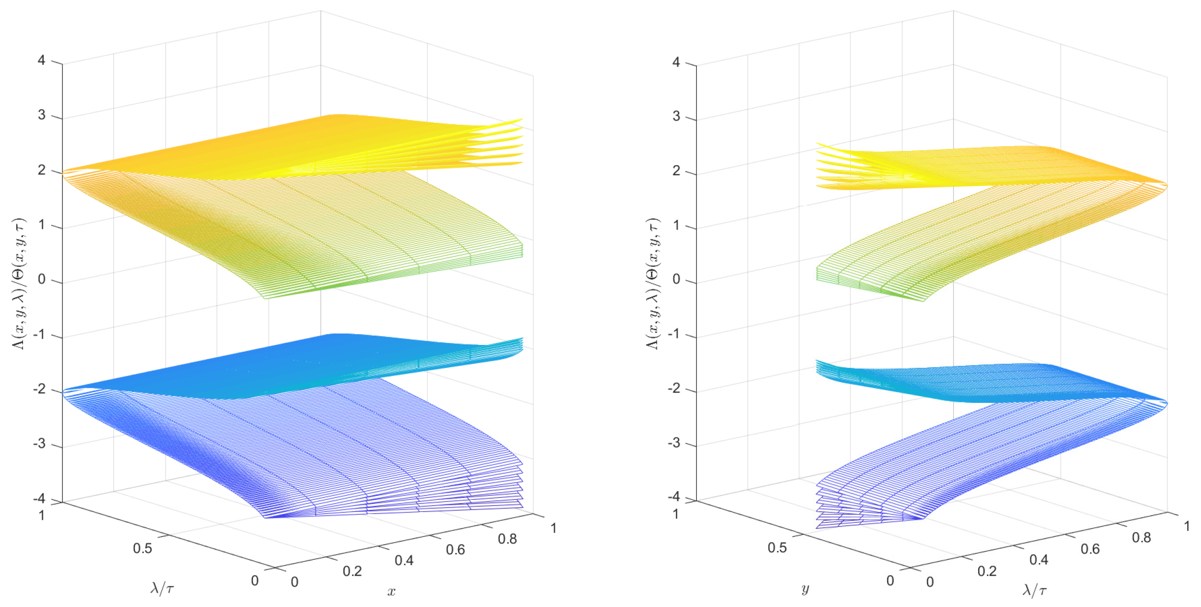
and
concerning which some
-cuts and
-cuts can be simulated; they are shown in
Figure 1 and
Figure 2. In
Figure 1, the top graph represents
and the bottom graph stands for
. The graph on the left shows how the solutions
and
vary with the independent variables
x and
(i.e.,
or
) when
y is fixed at five constants. The graph on the right shows how the solutions
and
change with the independent variables
y and
when
x is fixed at five constants. Moreover,
Figure 2 shows the numerical simulation of the level sets
and
as a function of
.
From
Figure 1 and
Figure 2, if the crisp number
c in the membership functions of the fuzzy numbers is known, then one can see that the image of the coupling solution and its level set change with the independent variable. However, we cannot get the image when
c changes continuously. This is worth improving.
Now we make clear that the condition
() in Theorem 2 holds and then prove the existence and uniqueness of the
-weak solution for (
26).
For briefness, letting
, then one has
which implies that
and so
Thus, based on Properties 21 of [
41], we know that the H-difference
exists.
From the foregoing proof, it follows that
and
Taking
then from Example 5.1 in [
26] we get
and
Similar to the above steps, one gets
and
which shows that the H-difference
exists.
It follows that
exists via Properties 21 of [
41], and
That is, the H-difference exists.
Therefore, in this case, (
26) has a unique
-weak solution in
.
Remark 7. From Example 1
, one can easily see that due to the “coupling” and the existence of the H-difference, it is more difficult to obtain the existence and uniqueness of the -weak solution of (
2)
with (
3).
This shows that it is challenging and valuable to obtain the results presented in Theorems 1
and 2.


