Fractals: An Eclectic Survey, Part-I

Abstract

Fractals are geometric shapes and patterns that may repeat their geometry at smaller or larger scales. It is well established that fractals can describe shapes and surfaces that cannot be represented by the classical Euclidean geometry. An eclectic survey of fractals is presented in two parts encompassing applications of fractals in a variety of diverse and innovative fields. The goal of the first part is to focus on the glossary of fractals, their mathematical description, aesthetic, artistic, and architectural applications, while the second part is focused on engineering, industry, commercial, and futuristic applications of fractals.

1. Introduction

Fractal geometry addresses itself to questions that many people have been asking themselves. It concerns an aspect of Nature that almost everybody had been conscious of, but could not address in a formal fashion. Fractal geometry seems to be the proper language to describe the complexity of many very complicated shapes around us.

Mandelbrot, (1990)

The term ‘Fractal’ was coined by Mandelbrot in 1975 to describe irregular geometries in nature and in mathematics that contain self-similarity. The name Fractal comes from the Latin word fractus, which means “broken” or “fractured”, and justified from the fact that there are self-similar parts within fractals.

Classical geometry is sufficient to understand many geometries in nature, but what about a fern, the silhouette of a tree covered in ice on a hill, the veins in a leaf, the intricate branching of our lungs, brain, or the geometric irregularity of a coastline? Euclidean geometry cannot provide simple descriptions of these shapes, but that does not mean they are without any intrinsic order. Most of them share a common property called self-similarity i.e., every small piece contains a copy of the whole shape, or at least a part of the whole that looks like it, and every smaller piece contains still smaller copies of the whole, and so on. With simple geometry we will learn how to grow basic fractals and how to understand the surprisingly simple rules that define the infinitely complex Mandelbrot set. We will see how to quantify the roughness of fractals and in what sense an object can have a fractal (non-integer) dimension. A crucial distinction between ‘mathematical fractals’ and ‘natural fractals’ is that it is possible to zoom in indefinitely on a mathematical fractal (e.g., Mandelbrot set, Julia sets, etc.) whereas in the case of natural fractals, a fractal description is valid only over a small range of scales (e.g., coastlines, clouds, etc.).

Broadly speaking, fractals are geometric shapes and patterns that may repeat their geometry at smaller (or larger) scales due to the inherent self-similarity present in the shape. This survey explores mathematical and natural fractals with the goal of providing an extensive review and state-of-the-art research, developments, and applications of fractals in two parts. The first part focuses on the glossary of fractals, their mathematical description, aesthetic, artistic, and architectural applications, while the second part is focused on engineering, industry, commercial, and futuristic applications of fractals. These applications range from aesthetic designs in art, fashion designing, landscape generation, tessellations, fractal image compression, design of fractal shaped antennas to other innovative and evolving fields of scientific and engineering research. We will explore several examples of fractals that are making a remarkable impact into technologies of today and will continue to contribute to the future.

Fractals can be generated using various algorithms and deals with objects that do not have integer dimensions. The earliest and standard examples of deterministic (mathematical) fractals include the Cantor set, the Koch curve, the Sierpinski triangle, the Mandelbrot set, and Julia sets. Contrary to their complicated geometry and infinitely complex patterns, fractals have found lot of use in real life applications over the past 2–3 decades.

We shall begin with the introduction to the most famous and iconic fractal, namely the Mandelbrot set, in Section 2. Basic mathematical concepts and the space in which fractals live are introduced to ensure that the reader is aware of the mathematics behind fractals, though the readers without decent mathematical background would also be able to follow the article without difficulties.

In Section 3, we consider the fractal dimension (which is a non-integer number for many fractal objects in contrast to the integer dimension of usual Euclidean objects), which provides a relative measure of the density of a fractal with respect to the space in which it lives. Several types of fractal dimensions existing in the literature are described here along with examples. The application of the fractal dimension to many diverse fields including coastlines and other natural objects is also discussed.

A tessellation or tiling is a collection of figures that fills the plane with no overlaps and no gaps. Fractals possess space filling properties, i.e., they can fill the spaces without gaps by placing self-similar copies together. Tilings have a long history and they appeared for decorations in many civilizations and cultures as the earliest examples. The classical text book by B. Grünbaum and G.C. Shephard [1] is by far one of the richest source on tilings containing a great deal of information. In Section 4, we provide a brief overview of the simple mathematics behind fractal tilings along with examples that can tile the Euclidean planes ${\mathbb{R}}^2$ and ${\mathbb{R}}^3$.

Section 5 is dedicated to artistic applications of fractals namely, fractal art. Fractal art is a genre of algorithmic art and digital art in which the results resemble the fractal objects or obey fractal properties. Fractal arts are also found in ancient times in manuscripts, hand-painted images, rugs, domes of mosques, and sculptures in old temples have patterns that are reminiscent of fractal art. So, fractals were designed even before they were discovered by Mandelbrot in 1970s and 1980s. We consider several application areas of the fractal art in coloring books, art galleries, ceramics, screensavers, calendars, and most excitingly in exploring infinity.

A recent application of fractals is seen in fractal clothing. Clothing is one of the most important factors for human survival and many clothing styles have emerged with improvements in technology. Clothing has huge market demand and a number of fashion brands have evolved over the years. Use of fractals in art grabbed the attention of researchers for their inherent features such as self-similarity, symmetry, pattern regularity, etc., and artists and designers started using fractal art in the designing of clothes. In Section 6, we discuss algorithms for generating fractal garment patterns and designs. Fractal clothing is becoming popular and in future it will open high avenues for research and development, investments, and styling.

In Section 7, we present flying fractals! The fractal-shaped hot air balloons were first designed and built by Jonathan Wolfe, executive director of the Fractal Foundation, an organization dedicated to inspiring interest in math and science through fractals. Two fractal balloons took to the sky at the Albuquerque International Balloon Fiesta in October 2013. Since then a number of fractal hot air balloons have been manufactured, which are also some of the largest fractals ever printed—they are discussed in Section 7 in more detail.

Short notes on applications of fractals in other emerging fields such as econophysics and military (for defense purposes) are given in brief in Section 8 and Section 9, respectively.

Several books and monographs are available on fractal geometry, its mathematical development, and applications. We particularly refer to the monograph entitled “Benoît Mandelbrot: A Life In Many Dimensions” [2], which is a collection of articles written by researchers who worked with Mandelbrot including mathematicians, physicists, biologists, economists, engineers, artists, musicians, and teachers, memorializing the remarkable breadth and depth of his work and accomplishments in science, engineering, and arts. Some articles in this monograph are very technical while others are entirely descriptive and every article include stories about Mandelbrot. We also refer to The Fractalist. Memoirs of a Scientific Maverick [3], the memoirs started by Mandelbrot and published later in the year 2012 post his demise. The book is oriented towards a narrative of Mandelbrot’s life and the amazing journey on how from a child in Warsaw he became a scientist at Yale University. For a unified list of almost all the works by Mandelbrot and others on fractal geometry we refer to [4]. Some additional book recommendations and fractal generating software are discussed in Section 10.

The entire manuscript is organized keeping in mind a wider spectrum of readers from academia and industry. This eclectic survey will enthrall and entertain the readers with the infinite complexity, beauty, and applications of fractals.

2. Space of Fractals and Iterated Function Systems

2.1. Space of Fractals

To understand fractals mathematically, we need some basic background. Let X be a non-empty set. Define a distance function $d:X\times X\to {\mathbb{R}}^{+}$ (which measures the distance between pairs of points x and y in X) by:

(i)

$d(x,y)\ge 0\mathrm{and}d(x,y)=0\iff x=y,\forall x,y\in X$

(ii)

$d(x,y)=d(y,x),\forall x,y\in X$

(iii)

$d(x,y)\le d(x,z)+d(z,y),\forall x,y,z\in X$.

The function d is called a metric on X and $(X,d)$ is called a metric space. Fractal geometry is the description, classification, analysis, and observations about subsets of metric spaces.

Definition 1.

A metric space $(X,d)$ is said to be complete if every Cauchy sequence ${\left\{x_n\right\}}_{n=1}^{\infty }$ of points in X has a limit in $x\in X$, i.e., $x_n\to x$ in X.

Definition 2.

Let $S\subset X$ be a subset of a metric space $(X,d)$. S is compact if every infinite sequence ${\left\{x_n\right\}}_{n=1}^{\infty }\in S$ has a convergent subsequence in S.

Definition 3.

Let $(X,d)$ be a complete metric space and $\mathcal{H}\left(X\right)$ be the set of non-empty compact subsets of X. $\mathcal{H}\left(X\right)$ is called space of fractals equipped with the Hausdorff metric h defined by: For any $A,B\in \mathcal{H}\left(X\right)$, distance between A and B is given by

$$h(A,B)=max\left\{d(A,B),d(B,A)\right\}$$

where, $d(A,B)={sup}_{x\in A}{inf}_{y\in B}\left\{d(x,y)\right\}$.

Any element of $\mathcal{H}\left(X\right)$ is a mathematical fractal and although classical Euclidean objects such as spheres, cubes are not considered as fractals but mathematically they are elements of $\mathcal{H}\left(X\right)$ and if there is no confusion likely to occur we can still consider them as fractals. We refer the reader to Barnsley (Chapter 2, [5]) for a proof of the fact that the space $\left(\mathcal{H}\right(X),h)$ is a complete metric space.

2.2. Iterated Function Systems and Attractors

Definition 4.

A transformation $w:X\to X$ on the metric space $(X,d)$ is called contractive or a contraction mapping if there is a constant $0\le \alpha <1$ such that

$$\begin{array}{cc}\hfill d\left(w\right(x),w(y\left)\right)& \le \alpha d(x,y)\forall x,y\in X.\hfill \end{array}$$

(1)

α is called contractivity factor of w.

Definition 5.

Let $(X,d)$ be a complete metric space. An iterated function system (in short IFS) is a finite set of contraction mappings $w_i:X\to X$, having contractivity factors ${\alpha }_i$, for $i=1,2,\dots ,m$. The number

$$\alpha =\underset{1\le i\le m}{max}{\alpha }_i$$

is called contractivity factor of the IFS.

Theorem 1.

Let $\{X,w_i:i=1,2,\dots ,w_m\}$ be an IFS with contractivity factor α. Then the transformation $W:\mathcal{H}\left(X\right)\to \mathcal{H}\left(X\right)$ defined by

$$\begin{array}{c}\hfill W\left(B\right)=\bigcup _{i=1}^m{w}_i\left(B\right)\end{array}$$

(2)

for all $B\in \mathcal{H}\left(X\right)$ is a contraction mapping on $\mathcal{H}(X,h(d\left)\right)$ with contractivity factor α. That is

$$h\left(W\right(B),W(C\left)\right)\le \alpha h(B,C)for allB,C\in \mathcal{H}\left(X\right).$$

Moreover, by contraction mapping theorem it has a unique fixed point $A\in \mathcal{H}\left(X\right)$, which satisfies

$$A=W\left(A\right)=\bigcup _{i=1}^m{w}_i\left(A\right)$$

(3)

and is given by $A={lim}_{n\to \infty }{W}^{\circ n}\left(B\right)$ for any $B\in \mathcal{H}\left(X\right)$. Here, $W^{\circ k}\left(B\right)$ denotes the usual $k-$fold composition of W.

Definition 6.

The fixed point A described in Theorem 1 is called the attractor of the IFS. Since $A\in \mathcal{H}\left(X\right)$, therefore, it is a fractal.

All examples of natural and manufactured fractals presented in this article are geometrically complex subsets of simple spaces such as ${\mathbb{R}}^2$ or ${\mathbb{R}}^3$ that belong to $\mathcal{H}\left(X\right)$ with $X={\mathbb{R}}^2\left(or{\mathbb{R}}^3\right)$.

2.3. Mandelbrot Set

Commenting on the sublime and geometrical complexity present in nature, in his famous book The Fractal Geometry of Nature (1982), Mandelbrot quoted, “Clouds are not spheres, mountains are not cones, coastlines are not circles, and bark is not smooth, nor does lightning travel in a straight line” [6].

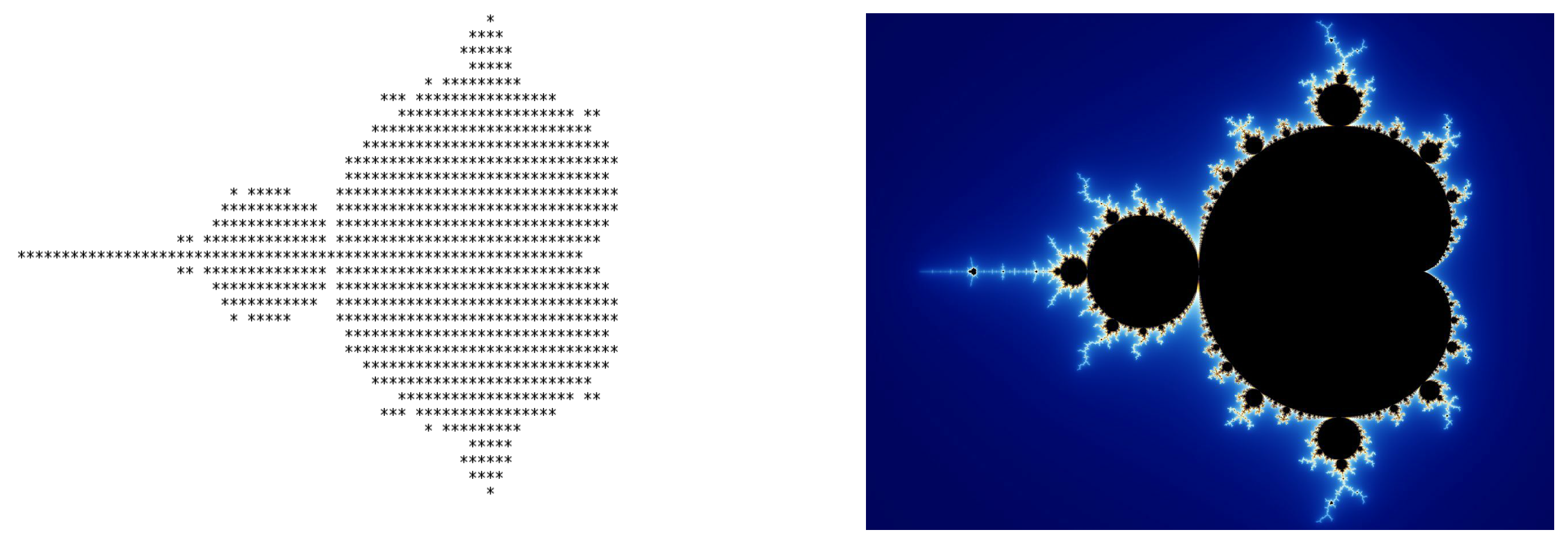
Before we explore fractals and their diverse applications, let us look at Benoît Mandelbrot’s eponymous set, which is the most iconic, complex, and visually entrancing fractal, popularly known as the Mandelbrot set (Figure 1) whose boundary is not only a fractal but much beyond our imagination (see Section 5 for more details).

Robert Brooks and Peter Matelski published the first image (Figure 1a) of the Mandelbrot set in 1978 describing it as the set of complex numbers c such that the function $f\left(z\right)=z^2+c$ has a stable periodic orbit. However, it was Mandelbrot who plotted the modern day image of Mandelbrot set with detailed geometry on 1 March 1980 at IBM (Figure 1b). This set is determined entirely by iterating the map

$$f_c\left(z\right)=z^2+c$$

where c is a complex number. The Mandelbrot set is the set of complex numbers c such that the sequence of numbers

$$f_c\left(0\right)=c,f_c^2\left(0\right)=f_c\left(f_c\left(0\right)\right)=c^2+c,f_c^3\left(0\right)=f_c\left(f_c\left(f_c\left(0\right)\right)\right)={(c^2+c)}^2+c,\cdots$$

remains bounded (does not escape to infinity). If after computing some terms we obtain a number big enough then we can stop. If after n steps, we have $\left|f_c^n\left(0\right)\right|>2$ then the sequence of numbers $f_c^n\left(0\right)$ escapes to infinity and c does not belong to the Mandelbrot set.

The Mandelbrot set is considered as one of the most engrossing discoveries of mathematics and the best known examples of mathematical visualization, self-similarities, beauty, and captivating patterns when we zoom on it. The Mandelbrot set has appeared on coffee mugs, T-shirts, tiles, balloons, utensils, and even in cinema and television commercials. More details on this exotic set will follow in later sections. The reader may refer to the book The Beauty of Fractals by Peitgen and Richter published by Springer (1986) specifically written for promoting the Mandelbrot set. There are many online videos available today, which gives incredible zooms on this set and we refer to [7] for a very interesting zoom.

3. Fractal Dimension

In classical Euclidean geometry, shapes are assigned integer dimension also called topological dimension. For instance, a line is a 1-dimensional object, a square is 2 dimensional, and a cube is a 3-dimensional object; however, this definition is not adequate to describe fractal objects. Fractal dimension is a (typically non-integer) number that can be associated with every natural, random, and manufactured fractal to measure or quantify the complexity of the fractal relative to the space in which it lives [5,8,9,10,11].

As mentioned before fractals model broken, complex, and irregular geometries; however, some shapes are more complex and irregular (e.g., coastlines) than others. The fractal dimension is used to quantify this complexity and roughness. There are many different variants of the fractal dimension such as the Hausdorff dimension (based on measures and the earliest also), similarity dimension (works well for self-similar objects), box-counting dimension (works for arbitrary objects and easy to implement on computers), and the divider dimension. They all are equal for exactly self-similar fractals such as the Koch curve, Sierpinski triangle, etc.

Mandelbrot conjectured in 1985 that the Hausdorff dimension of the boundary of the Mandelbrot set is 2, which was proved by Shishikura [12] using the concept of bifurcation of parabolic periodic points. For a complete treatment of Hausdorff dimension we refer to the book by Edgar [13]. Hausdorff dimension is the best way to measure fractal dimension of a bounded subset of ${\mathbb{R}}^n$ since it considers all the possible coverings (of a given diameter) that the bounded subset may admit, and it possesses better analytical properties than the box dimension. We refer to the works of Fernández-Martínez et al. [14,15,16,17] who proposed a way to deal with the calculation of Hausdorff dimension in applications for compact Euclidean subsets including the higher dimensional case in more general settings. Their approach combines both theoretical results along with techniques from machine learning, thus leading to the first-known attempt to calculate Hausdorff dimension in applications. The reader may also refer to the classical text books by Barnsley [5], Falconer [8], and the book by Frame et al. [9] for a collated study of various types of fractal dimensions.

3.1. Basic Definitions and Results

Definition 7.

Let $(X,d)$ be a metric space and A be a compact subset of X. Let $ϵ>0$, (a small number) is given, define

$$N_{ϵ}\left(A\right)=minimum number of closed balls which covers A$$

i.e., ${\displaystyle A\subset \bigcup _{i=1}^{N_{ϵ}}{B}_{ϵ}\left(x_i\right)}$, where $B_{ϵ}\left(x_i\right)$ is a ball of radius ϵ centered at $x_i$. We say that A has fractal dimension $D\left(A\right)$ or simply D if

$$\begin{array}{c}\hfill D=\underset{ϵ\to 0}{lim}\frac{log\left(N_{ϵ}\left(A\right)\right)}{log\left(\frac{1}{ϵ}\right)}\end{array}$$

(4)

provided the limit exists.

We cite two important results from Barnsley [5]. The first theorem replaces the continuous variable $ϵ$ in Equation (4) by a discrete variable to simplify computations and the second theorem is an existence result on fractal dimension.

Theorem 2

(Theorem 1.1, Chapter 4 [5]). Let A be a compact subset of a metric space $(X,d)$. Let ${ϵ}_n=C{r}^n$ for each real number $0<r<1$ and $C>0$. Then A has fractal dimension D given by

$$D=\underset{n\to \infty }{lim}\left\{\frac{log\left(N_{{ϵ}_n}\left(A\right)\right)}{log\left(\frac{1}{{ϵ}_n}\right)}\right\}.$$

(5)

Theorem 3

(Theorem 2.1, Chapter 4 [5]). Let m be a positive integer. Consider the space $\left({\mathbb{R}}^m,Euclidean\right)$. Then $D\left(A\right)$ exists for all $A\in \mathcal{H}\left({\mathbb{R}}^m\right)$. If $B\in \mathcal{H}\left({\mathbb{R}}^m\right)$ such that $A\subset B$, then $0\le D\left(A\right)<D\left(B\right)\le m$. Here, $\mathcal{H}\left({\mathbb{R}}^m\right)$ is the set of all non-empty compact subsets of ${\mathbb{R}}^m$.

3.2. Similarity Dimension

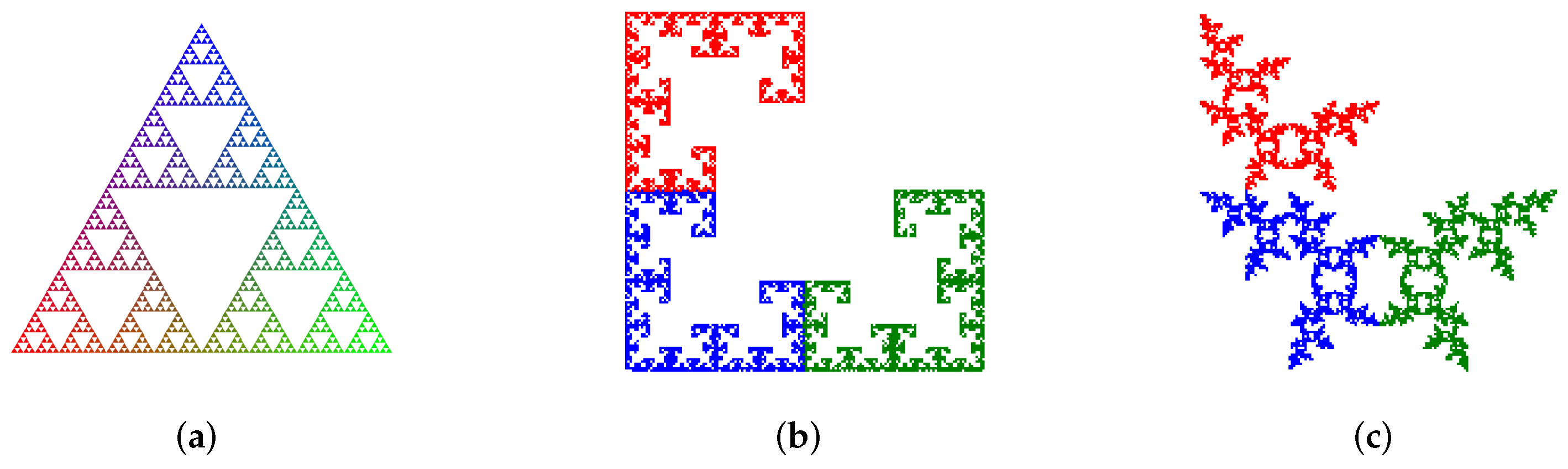
Definition 8.

For self-similar fractals made of N copies, each scaled by the same factor $r<1$, the similarity dimension $D_s$ is given by

$$\begin{array}{c}\hfill D_s=\frac{log\left(N\right)}{log\left(\frac{1}{r}\right)}.\end{array}$$

(6)

The Sierpinski gasket (Figure 2a) is a well-known self-similar fractal made up of 3 copies of itself each scaled by a factor $\frac{1}{2}$. Therefore, $D_s=\frac{log\left(3\right)}{log\left(2\right)}=1.58496$.

The fractals in Figure 2b,c also consist of $N=3$ pieces each scaled by $r=\frac{1}{2}$, so they have the same similarity dimension as that of Sierpinski gasket; however, neither looks like the gasket, nor do they look like one another. This shows that the similarity dimension does not fully characterize all fractals.

Table 1. Similarity dimensions of some well-known fractals.

S. No.	Fractal	Name	Similarity Dimension	No. of Copies (N) and Scaling Factor (r)
1		Straight line	1.00000	$N=1$, $r=1$
2		Cantor set	0.63100	$r=\frac{1}{n}$ at the $n\mathrm{th}$ step of construction
3		Koch curve	1.26186	$N=4$, $r=\frac{1}{3}$
4		Box fractal	1.46497	$N=5$, $r=\frac{1}{3}$
5		Sierpinski Triangle	1.58496	$N=3$, $r=\frac{1}{2}$
6		Sierpinski pentagon	1.67228	$N=5$, $r=\frac{1}{2-\sqrt{5}}$
7		Sierpinski carpet	1.89279	$N=8,r=\frac{1}{4}$
8		Twin dragon	2.00000	$N=2,r=\frac{1}{\sqrt{2}}$
9		Terdragon	2.00000	$N=3$, $r=\frac{1}{\sqrt{3}}$
10		Eisenstein fractions	2.00000	$N=4,r=\frac{1}{4}$
11		Koch snowflake	2.00000	$N=7$, six copies scaled by $\frac{1}{3}$ and one by $\frac{1}{\sqrt{3}}$
12		Lévy dragon	2.00000	$N=2$, $r=\frac{1}{\sqrt{2}}$

summarizes the similarity dimensions (in increasing order of magnitude) of some important fractals studied in the literature.

There is another definition of the similarity dimension for exactly self-similar objects, which is more inclusive and take into account fractals with different scaling factors.

Definition 9.

Let n be the number of scaled down pieces in the construction of a self-similar fractal and let $r_1,\cdots ,r_n$ be the scaling factors (some of them can be equal). Then, the similarity dimension $D_s$ is the solution of

$$\sum _{i=1}^n{r}_i^{D_s}=1.$$

(7)

This definition allow us to compute fractal dimension by solving the purely algebraic Equation (7) also known as the Moran’s equation. For the Koch curve, the similarity dimension is the solution of

$$\sum _{i=1}^4{\left(\frac{1}{3}\right)}^{D_s}=1,$$

which gives $D_s=1.26186$, same as calculated earlier. The similarity dimension works well for exactly self-similar fractals, but many objects including coastlines, borders are not self-similar.

There are some other dimensions such as packing dimension (based on packing measure), mass dimension, covering or Lebesgue dimension, Miknowski dimension, and few others and most of these provide different means of approaching and computing fractal dimension, and each type of dimension can yield a slightly different value. Nevertheless, they satisfy some standard relationships, for example

$$D_h\le D_b,\mathrm{and}{D}_h\le D_s$$

where $D_h$ denotes the Hausdorff dimension with equality possible if the open set condition (OCS) holds (see Section 4.1 for definition of OSC). Some other properties such as monotonicity, stability, invariance, etc., are also satisfied by all of these and we refer to [13] (Chapter 6) for more details and results on these dimensions.

3.3. Fractal Dimension of Coastlines

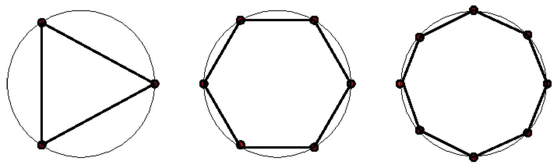
The standard approach for measuring the length L of a curve C is to approximate the curve by line segments of length r. If there are N of these segments at this scale, the length of the curve is $L=N\times r$. For example, the three images in Figure 3 show approximations of the circumference of the unit circle by 3, 6, and 8 segments of equal length. It is clear that as the number of segments increases, the line segments approximate, $2\pi$ very closely, the actual circumference of the circle.

This method works for smooth curves, but the problem is that natural fractals such as coastlines and rivers are not made up of smooth Euclidean curves that can be approximated in this way.

The divider (or compass) dimension is another fractal dimension that examines both the relationship between scaling size and the length of a curve and the relationship between scaling size and the number of segments that are needed to cover the curve at a given size. This dimension is useful for calculating fractal dimension and the length of coastlines, rivers, and other natural objects.

Suppose we wish to find the fractal dimension of a coastline (an irregular curve). Choose a step length $ϵ$ and is walked along the coastline until the end is reached. Let $N\left(ϵ\right)$ be the number of steps taken to reach the end. The length of the coastline is then $L\left(ϵ\right)=ϵ·N\left(ϵ\right)$. For a large $ϵ$, this method skips many irregularities along the coastline, but as $ϵ$ decreases, the finer features of the coastline are also included, and the overall length increases. Richardson was the first to use the divider method in his work on coastlines [18] and showed that this behavior is a power law defined by

$$L\left(ϵ\right)=k\times {ϵ}^{\alpha }\mathrm{where}k,\alpha \mathrm{are} \mathrm{constants}.$$

(8)

Mandelbrot [19] later discovered that $\alpha =1-D$ where D is the similarity dimension. Thus, $L\left(ϵ\right)=k\times {ϵ}^{1-D}$. Upon taking the logarithm of both sides, we obtain

$$logL\left(ϵ\right)=logk+(1-D)logϵ.$$

(9)

A plot between $log\left(ϵ\right)$ and $logL\left(ϵ\right)$ results in a line with approximate slope $1-D$. These plots of coastline length versus the step length are called Richardson plots. Thus, the power law behavior results in linearity on a double logarithmic plot (also called as $log-log$ plot). The resulting value of D is called the divider dimension.

Though, the data from length measurements of natural fractals are not exactly linear, but the approximation is good enough to use the least squares or regression method for a very good linear fit. Richardson used this technique when he observed the power–law behavior with the coastline of Great Britain [18].

It follows that $ϵ\times N\left(ϵ\right)=k\times {ϵ}^{1-D}$ so that $N\left(ϵ\right)=k\times {ϵ}^{-D}$. This gives

$$logN\left(ϵ\right)=logk-Dlogϵ.$$

(10)

When using a double logarithmic plot, the slope of the resulting line will be approximately $-D$. Thus, there are two ways to calculate the divider dimension from Equations (9) and (10), and the values of D are still roughly the same although there can be some deviation because of the different methods used.

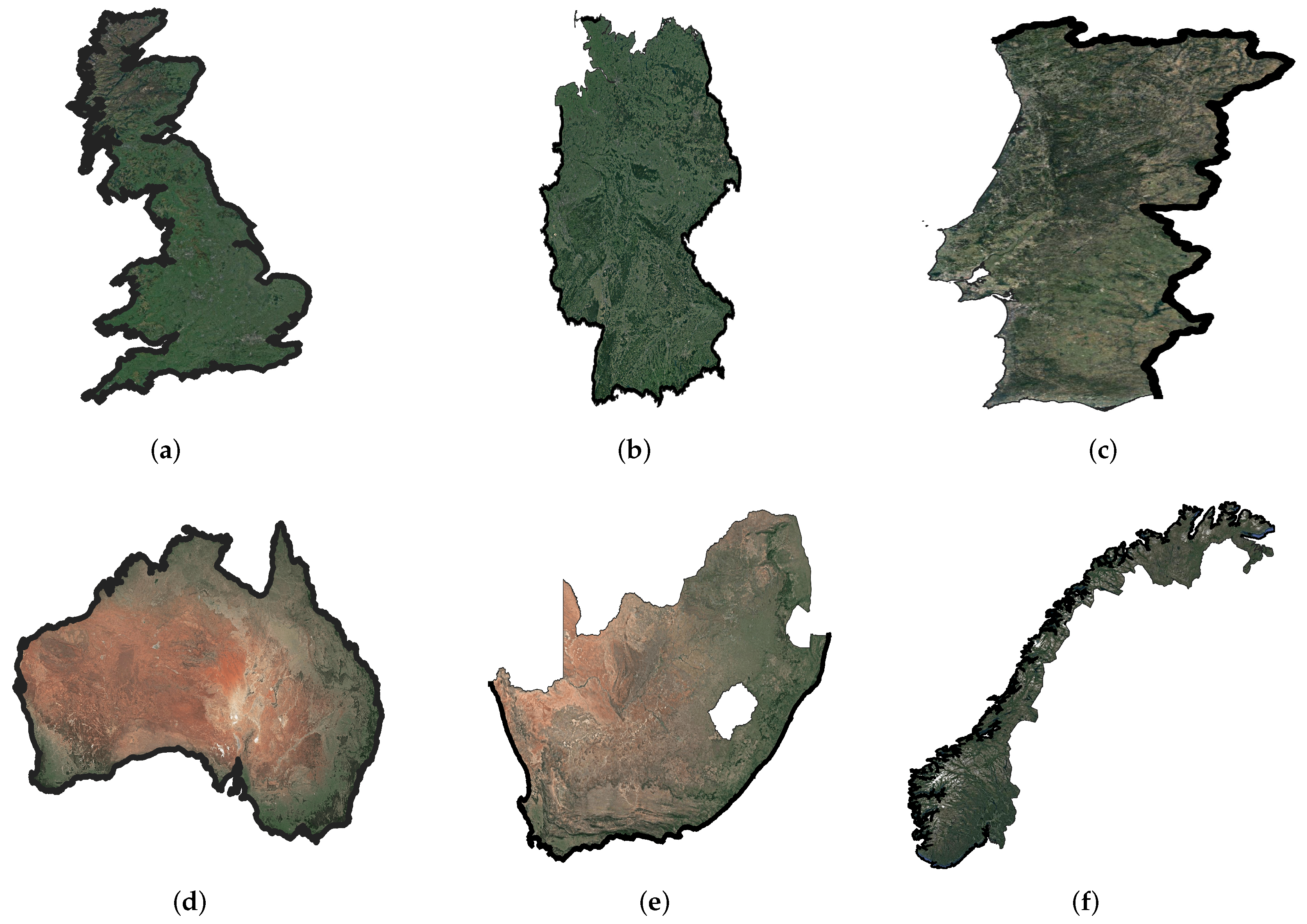
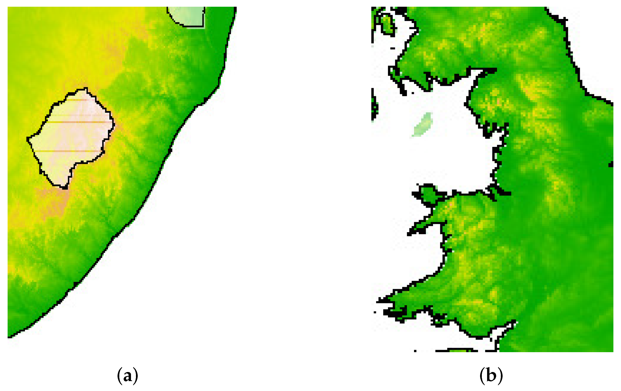
Coastlines (such as clouds, river networks) exhibit self-similarity over a range of scales, which is expected because the forces that shape coastlines, e.g., wind, tides, erosion, etc., operate in approximately the same way over a wide range of scales. Figure 4 shows some coastlines and borders (created in QGIS software, Pi-version) which have been focus of interest by several authors. For clarity, we have marked the border/coastline of interest with thick black color.

The fractal dimension D of a coastline measures the geometric irregularity and extent of coastlines and its value increases (but remain between 1 and 2) with increasing irregularity. The coastline with lower D value are more smoother. Different methods have been proposed in the literature to estimate the fractal dimension of coastlines, including the divider method, the box-counting method, the stochastic noise method, etc., (see [10,11,18,19] and reference therein).

Richardson was the first to observe and described the coastline paradox (which states that the length of a coastline depends directly on the length of the scale used for the measurement) between the length of coastlines and scale size [18]. Richardson noticed that the Spanish/Portuguese border was stated as 1214 km by Portugal 987 km by Spain, a difference of 227 km. This dispute could now be explained by the fact that the two countries measured their border using different measurement scales. This was the beginning of coastline paradox.

Richardson plotted $log\left(L\right)$ vs. $log\left(r\right)$, obtaining points approximately along straight lines with slopes given in

Table 2. Slopes obtained by Richardson (1961) and fractal dimension (D) calculated by Mandelbrot (1967).

S. No.	Coastline	Slope	Fractal Dimension (D)	Reference Figure
1	West coast of Britain	$-0.25$	$1.25$	Figure 4a
2	Land frontier of Germany	$-0.15$	$1.15$	Figure 4b
3	Land frontier of Portugal	$-0.14$	$1.14$	Figure 4c
4	Coastline of Australia	$-0.13$	$1.13$	Figure 4d
5	Coast of South Africa	$-0.02$	$1.02$	Figure 4e

. Richardson wrote that the slopes of the $log-log$ plots “may be expected to have some positive correlation with one’s immediate visual perception of the irregularity of the frontier”. The slope of the line was found $1-D$ (by Mandelbrot), which on solving for D, gives the values in Table 2.

For Great Britain, $1-D=-0.25$, so that the fractal dimension of Great Britain is $1.25$. For the coastline of South Africa $D=1.02$ and so on. Mandelbrot interpreted this value of D as fractal dimension in [11].

In general, a more irregular coastline will give rise to a steeper slope, which results in a large value of the fractal dimension as compared to a regular coastline that will have a comparatively small dimension. Indeed, as seen in the same-scale Google Maps images of Figure 5, the coast of South Africa is very smooth and the west coast of Britain is very rough. This was one of the first instances where physical objects were seen to have non-integer dimensions.

3.4. Box-Counting Dimension

A major difficulty in working with the divider method is that a coastline (or curve) may have multiple forward intersections at a particular stepsize, so how to cover those and there are always some leftover portions of the coastline (or curve) that have length less than the chosen scale. When the scale is is small, so is the error, but at large scales we will make greater errors.

To circumvent these difficulties another variant of fractal dimension known as the box-counting dimension $D_b$ can be used. $D_b$ is also an exponent in a power–law relation exactly as the similarity dimension $D_s$. This is one of the most popular and commonly dimension because of its implementation simplicity and it can be applied to any object in nature. It is a simplification of the Hausdorff dimension, and for many fractals the box-counting dimension is equal to the other fractal dimensions; however, there are objects for which it can differ from other fractal dimensions. For example, the box-counting dimension of the set of rational numbers is 1 whereas the Hausdorff dimension is 0 [8].

Different versions of the box-counting dimension are defined in the literature and we start with a particular case of Theorem 2, we have the box-counting theorem (Barnsley [5]).

Theorem 4

(The Box Counting Theorem). Let A be a closed and bounded subset of ${\mathbb{R}}^2\left({\mathbb{R}}^3\right)$. Cover ${\mathbb{R}}^2\left({\mathbb{R}}^3\right)$ by square boxes of side length $\frac{1}{2^n}$. Let $N_n\left(A\right)$ be the number of boxes that intersect A. Then the box counting dimension of A is given by

$$D_b\left(A\right)=\underset{n\to \infty }{lim}\left\{\frac{log\left(N_n\left(A\right)\right)}{log\left(2^n\right)}\right\}.$$

(11)

A novel theory that generalizes the classical box-counting dimension and fractal dimension to any space equipped with a fractal structure is given by Fernández-Martínez and Sánchez-Granero (2014), which include Theorem 4 as a particular case. The reader may also refer to the book by Frame et al. [9] for a summary and many examples of various types of fractal dimensions.

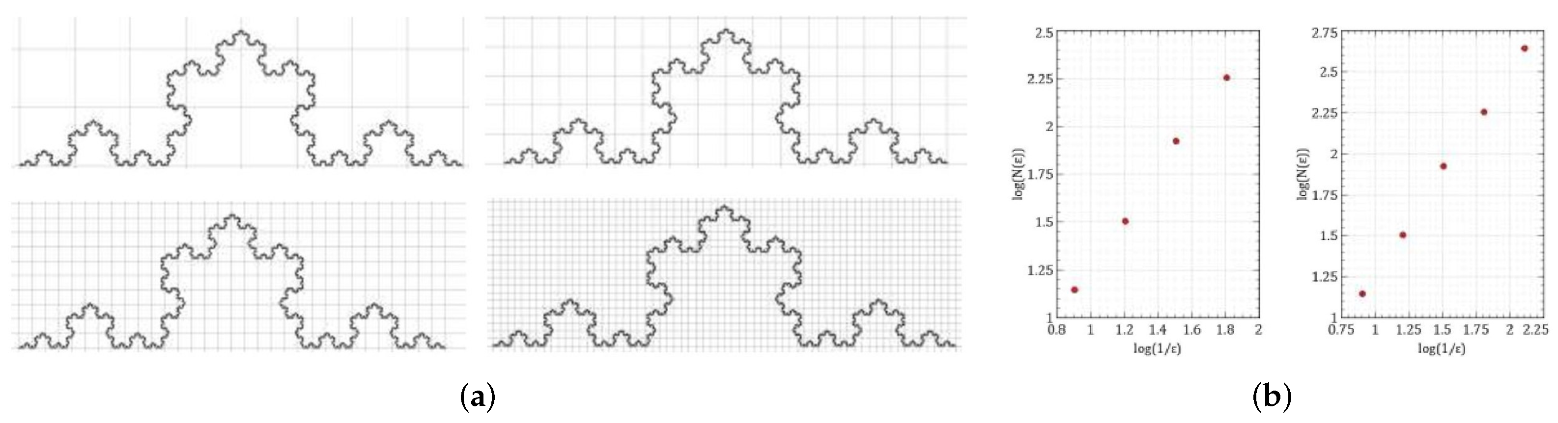
In Figure 6, the box counting method is applied to calculate the fractal dimension of the Koch curve with squares of four sizes and the box counting dimension turns out to be $D_b=1.2486$. Using five levels of box size (Figure 6b) gives $D_b\approx 1.2545$; however, since the Koch curve is self-similar we should expect $D_b$ to be exactly same as $D_s=1.26186$ (computed before). This can be achieved using one or two more levels of smaller boxes as they can detect more details.

Box-counting involves covering the object with the minimum number of boxes of side length $ϵ$ and finding how the number of boxes $N\left(ϵ\right)$ scales with $ϵ$. We now focus on box-counting dimension ($log-log$ approach) of rough or complex geometries (say) for example, a GoogleMap view of a coastline or a river. A step size $ϵ$ is chosen and a grid with boxes of size $ϵ\times ϵ$ is drawn on the given curve. The number of boxes $N\left(ϵ\right)$, which intersect the curve are counted for decreasing values of $ϵ$. A plot of $N\left(ϵ\right)$ vs. $ϵ$ on a double logarithmic scale is typically linear with slope $-D_b$. The number $D_b$ is called the box-counting dimension. The scaling hypothesis is that $N\left(ϵ\right)$ is related to $ϵ$ by a power law,

$$N\left(ϵ\right)=k·{\left(1/ϵ\right)}^{D_b}$$

(12)

which gives,

$$log\left(N\left(ϵ\right)\right)=D_{b}log\left(\left(1/ϵ\right)\right)+logk.$$

(13)

Thus, there are two ways for computing $D_b$, depending on the kind of information we have about $N\left(ϵ\right)$. For some objects (self-similar or not), we can find an exact formula for $N\left(ϵ\right)$. In this case, $D_b$ is computed using Theorem 4. For physical fractals and random mathematical fractals, an exact formula for $N\left(ϵ\right)$ may not be available. In such cases, $D_b$ can be computed by measuring the slope of the line in Equation (13). The later approach is used for computing fractal dimension of natural objects.

Recently, a multicore parallel processing algorithm has been proposed by Husain et al. and implemented to compute the fractal dimension of Australia [10] and India [20] using the box-counting method. This algorithm is the first to compute fractal dimension of coastlines in a parallel environment and can be used in computing fractal dimension of large coastlines (e.g., Canada, Indonesia, etc.) by exploiting the scalable, parallel structure of the algorithm. Applications of fractals dimensions have also been investigated by a number of researchers and we refer to the papers [10,21,22] and references therein for detailed analysis of various methods proposed for calculating fractal dimension in many other exciting fields of research.

3.5. Summary

We summarize this section with a brief note on important applications of fractal dimension. Several real world phenomenon exhibit statistical fractal properties and fractal dimension estimation has found applications in astronomy (e.g., in observing and analyzing turbulence in terrestrial bodies), acoustics (e.g., in automatic speech recognition using fractal dimension of speech sounds), earth sciences (e.g., in predicting compressive strength of volcanic welded bimrocks), diagnostic imaging (e.g., in characterizing cells and tissues, ophthalmology), electrochemistry (e.g., in the study of electrochemical reactions), image analysis, biology and medicine, neuroscience (e.g., in treatment of Alzheimer’s and brain related diseases), physics (e.g., in evaluating fractal dimension of profiles), and network analysis.

4. Fractals in Tessellation

A tessellation or tiling (also called rep tile) of the plane is the covering of the plane using one or more geometric shapes, called tiles, with no overlaps and no gaps. Tilings appear among the earliest decorations in many civilizations and cultures.

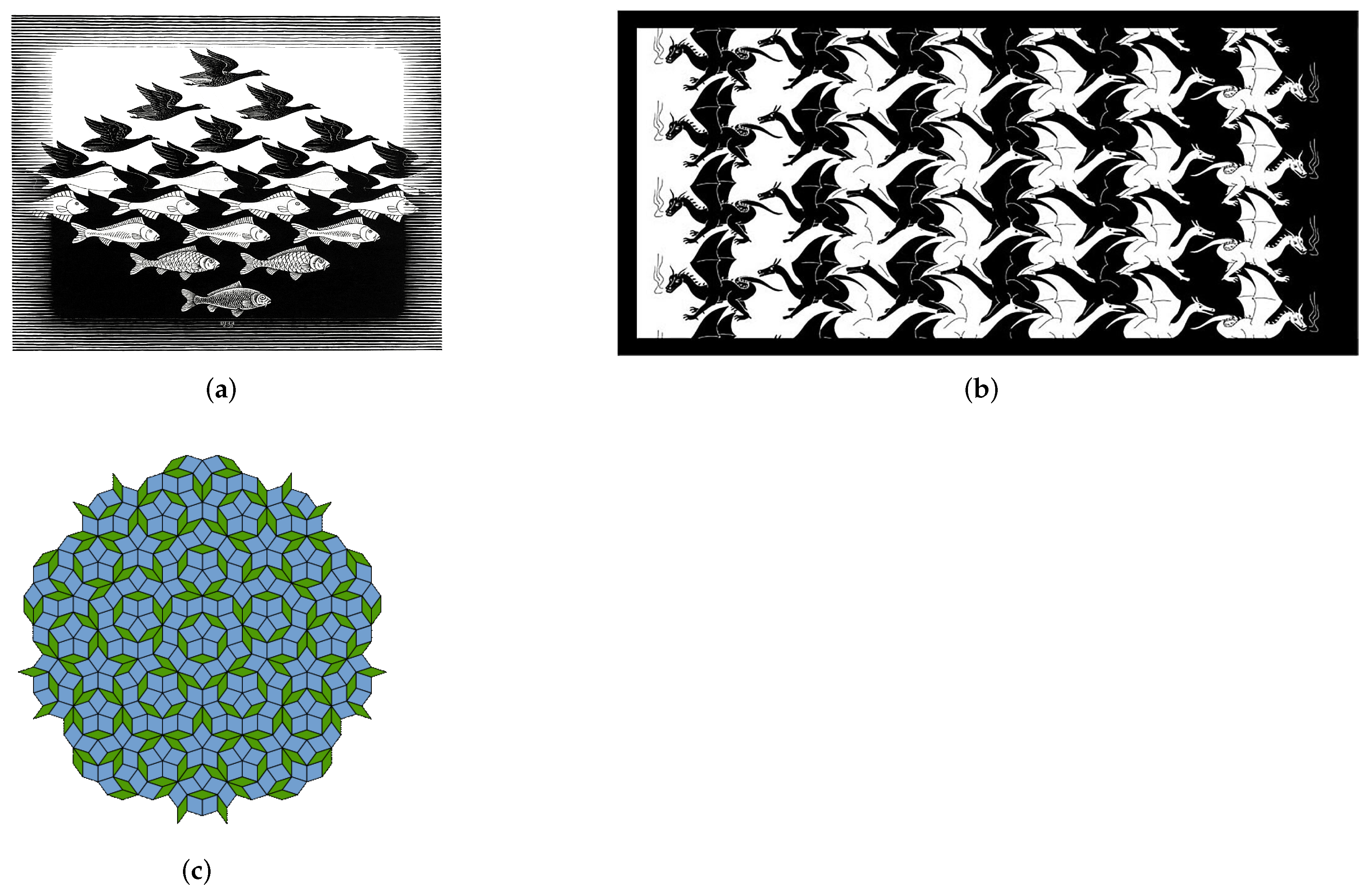
Notable tessellations artists M.C. Escher (also known as the King of Tessellations), Robert Fathauer (an electrical engineer) and Roger Penrose (a geometer, recreation mathematician, and the Physics Nobel prize winner (2020)) have fascinated people all over the world by their work on tessellations. A few examples of tessellations by these artists are shown in Figure 7. We also refer the reader to the classical text book by B. Grünbaum and G.C. Shephard [1] for an extensive study of tilings and patterns.

Tessellations can be broadly classified into fractal and non-fractal tessellations. Non-fractal tessellations are more closely related to the artistic world (for example, Figure 7a,b and designs in tile flooring, designs on furniture, etc.) whereas fractal tessellations are mathematical in nature and involve art as well (for example, Figure 7c, manmade fractals, etc.). Both the tessellations fill shapes using self-similarity. Major difference between the two types of tessellations is that non-fractal tessellations repeat geometric shapes that touch each other on a plane whereas fractal tessellations repeat shapes that have hundreds and thousands of different shapes of complexity. The space around the shapes sometimes (but not always) become shapes in the design. The space around shapes in non-fractal tessellations become repeating shapes themselves and play a major part in the design. Thus, a non-fractal tessellation is more closely linked to the artistic world, whereas a fractal tessellation is more mathematical in nature.

Rep tiles were introduced in 1963 as recreational objects by Gardner (1963) and Golomb (1964). In the 1980s they became interesting as models of quasicrystals [1], and as examples of self-similar fractals [5].

Fractal rep tiles are simply the rep tiles with fractal boundary. Computer generated drawings of tilings of the plane by self-similar fractal rep tiles appeared in the papers beginning 1980s and 1990s, for example the lattice tiling of the plane by copies of the twindragon. We refer to the works of several authors [23,24,25,26,27,28,29,30,31] for the study of fractal rep tiles.

We also refer to the recent works on fractal tilings by Bandt and Mekhontsev [32,33,34,35] for a comprehensive summary and current state of the art in the subject. The use of the inverses of integer matrices in the study of tilings is well-established, and can be found in particular in many of the references cited above.

Despite plenty of research on fractal tilings in 2D, very limited work is focused on the geometry of fractal rep tiles in 3D. In 3D, visualization is difficult and various topological properties of 3D fractal rep tiles such as interior points, boundaries, connectedness, simple connectedness, self-similarity, etc., cannot be answered simply looking at the pictures. Some of these properties in two dimensions are already discussed by many authors [28,29,31,36,37,38]. We refer to the pioneering work by Bandt [39] for the corresponding partial answers in 3D and directions for further research using the universal tool of neighbor graph.

4.1. Mathematics of Tiling

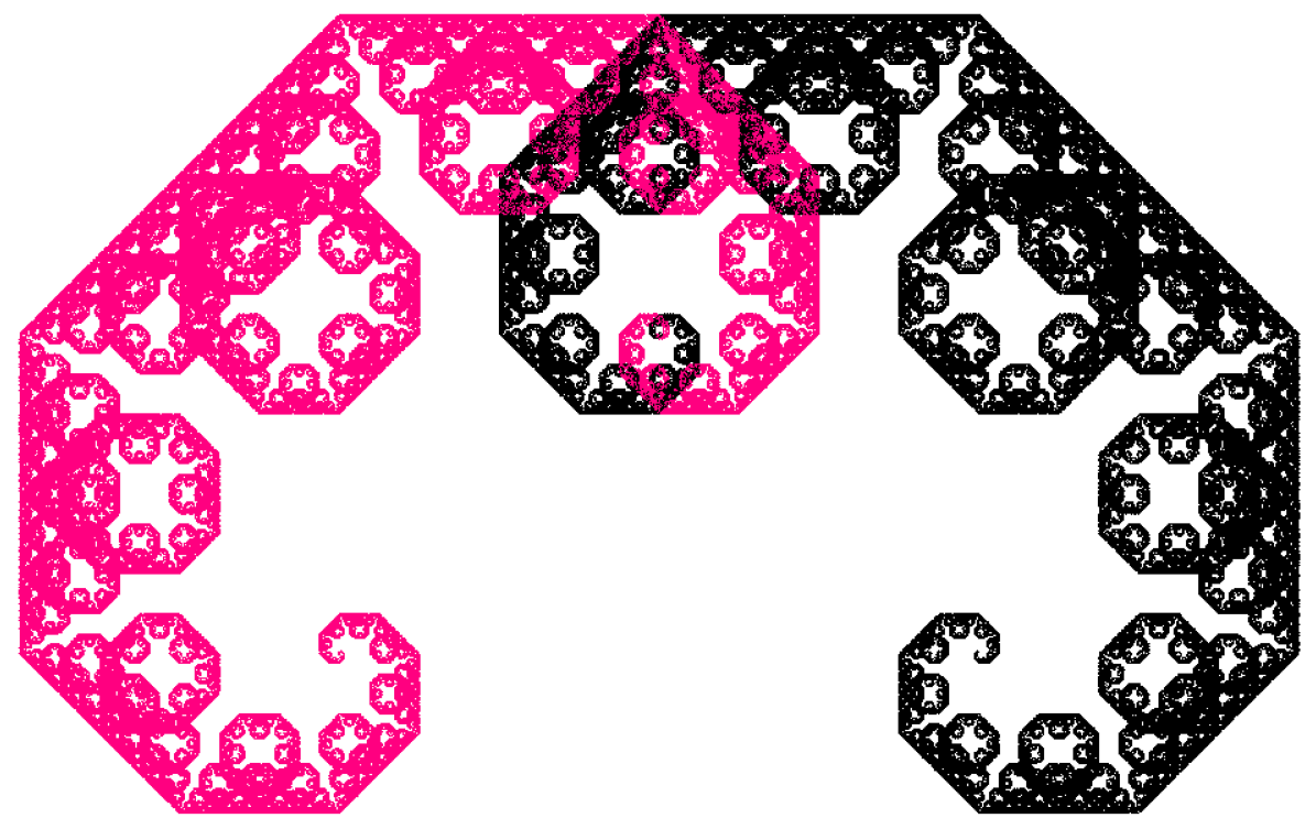
Paul Lévy tiled the plane with the classical fractal namely the Lévy dragon shown in Figure 8. This is indeed intriguing that the Euclidean plane can be tiled by this exotic curve having infinitely many holes, and from the picture, it is not obvious that it has any interior points.

Let us recall from Section 2, that by $\mathcal{H}\left(X\right)$ we mean the space of fractals containing non-empty compact subsets of X.

Definition 10.

A covering of a subset $A\in X$ is a set of open sets $\mathcal{C}=\{C_1,C_2,\dots ,C_n\}\in X$ whose union contains A., i.e.,

$$\begin{array}{c}\hfill {\displaystyle A\subset \bigcup _{i=1}^n{C}_i.}\end{array}$$

(14)

Definition 11.

A tiling of the plane is a countable family $A_i$ of compact sets that covers the plane with $int\left(A_i\right)\cap int\left(A_j\right)=\varnothing$ for $i\ne j$. Here, $int(·)$ denotes the interior of a set. Thus, the interior of any set in a tiling does not intersect the interior of any other set, i.e., tilings will have no overlap.

A chessboard is an elementary example of a self-similar tiling, which is composed of smaller tiles (called fractiles or rep tiles) of the same size, each having the same shape as the whole. Each tile in the chessboard is the scaled and translated image of the entire board.

Definition 12.

A closed set A in ${\mathbb{R}}^d(d=2,3)$ with nonempty interior is called an $m-$rep tile if there are sets $A_1,\dots ,A_m$ congruent to A, such that $int{A}_i\cap int{A}_j=\varnothing$ for $i\ne j$ and

$$g\left(A\right)=A_1\cup A_2\cup \dots A_m,$$

where g is a similarity mapping.

An important property of an IFS is the open set condition, briefly denoted as OSC, which controls the overlap of the sets $A_i$.

Definition 13.

Let $\{X,w_i:i=1,2,\dots ,m\}$ be an IFS. The IFS is said to satisfy open set condition, if there exists a non-empty open set $U\subset {\mathbb{R}}^n$ such that

$$\bigcup _{i=1}^m{w}_i\left(U\right)\subseteq U,w_i\left(U\right)\cap w_j\left(U\right)=\varnothing fori\ne j.$$

(15)

When the OSC holds and A has non-empty interior then A is a tile. Thus,

$${\mathbb{R}}^n=A_1\cup A_2\cup A_3\cup \dots$$

where each $A_i=h_i\left(A\right)$ is a copy of A by some affine map $h_j$, and the intersection $A_i\cap A_j$ of any two different copies has empty interior. The OSC has many equivalent formulations and is accepted as a natural separation condition for self-similar fractals [40].

For the Lévy curve in Figure 8, we have $m=2$, and the mappings are $w_1=g^{-1}{h}_1,w_2=g^{-1}{h}_2$ where

$$g\left(\mathbf{x}\right)=M\mathbf{x},M=\left[\begin{array}{cc}1& -1\\ 1& 1\end{array}\right],h_1\left(\mathbf{x}\right)=\mathbf{x}+\left[\begin{array}{c}0\\ 0\end{array}\right],h_2\left(\mathbf{x}\right)=\left[\begin{array}{cc}-1& 0\\ 0& 1\end{array}\right]\mathbf{x}+\left[\begin{array}{c}1\\ 1\end{array}\right],\mathbf{x}=\left[\begin{array}{c}{x}_1\\ x_2\end{array}\right].$$

The Lévy dragon in Figure 8 fulfills the OSC and is a $2-$rep tile but this was not so obvious even to its discoverer Paul Lévy. It was only after the year 2000 that the dimension of its boundary was calculated as $1.97$.

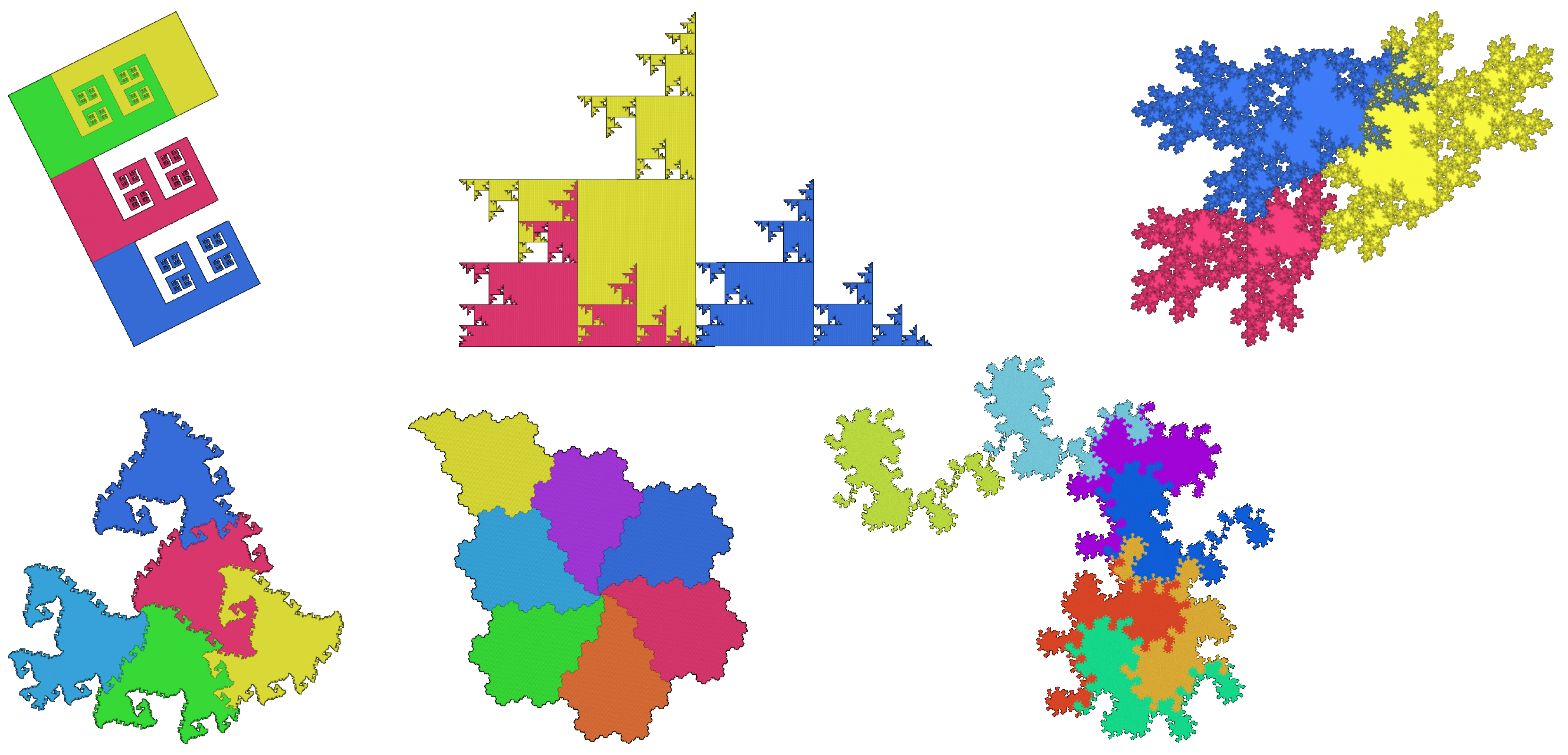
‘Rep’ stands for ‘replication’, and the sets are called tiles since they can tile the whole plane. For the plane, plenty of $m-$rep tiles are known for every m. Figure 9 shows some examples of $m-$rep tiles for different values of m [35,41].

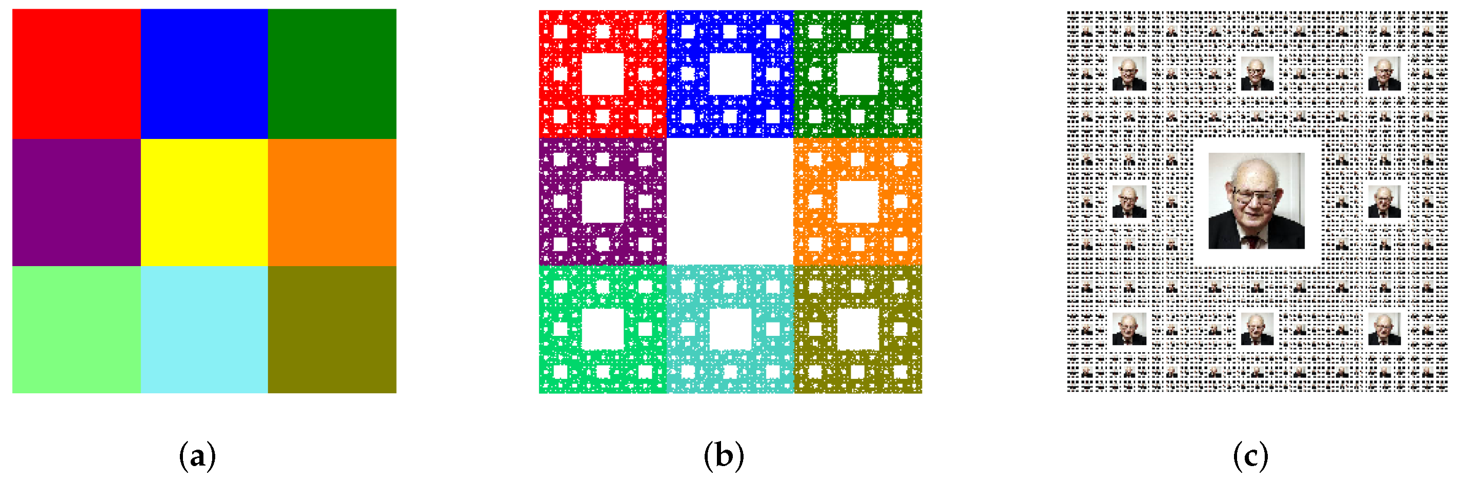
The standard carpet (box) tile is shown in Figure 10a. By removing the middle square from the box tile and repeating the same procedure recursively to the remaining eight subsquares we obtain the well known Sierpinski carpet in Figure 10b as the limiting set. Rather than removing the middle square, if we replace it with an image and iterate then we obtain the mathematical complement (inverse image) of the Sierpinski carpet. The Mandelbrot image carpet in Figure 10c is obtained by this procedure created in four iterations, resulting in $1+8+8^2+8^3+8^4=4681$ copies of the Mandelbrot image in the picture. Usually a circular or square logo or any other image, which fits in place of the removed square from the center of the Sierpinski Carpet will produce the best result for viewing.

Some more examples of well known as well as new fractal rep tiles are shown in Figure 11. All these rep tiles are obtained using the IFS construction kit package [42]. The interested reader may explore the IFS Kit for constructing exotic examples of fractal and rep tiles in ${\mathbb{R}}^2$ and the IFSTile package [41] for fractal and rep tiles in ${\mathbb{R}}^2$ and ${\mathbb{R}}^3$.

4.2. Fractal Rep Tiles in ${\mathbb{R}}^3$

The topological structure of fractal tilings in ${\mathbb{R}}^3$ can be very complex. Another challenge is that the OSC (a natural separation condition, which expresses geometric as well as measure-theoretic properties of tilings, see Definition 7), which controls the overlap of the $A_i$ may not hold for attractors that are made up of $A_i,1\le i\le m$ even if there is a one point intersection [40]. Moreover, it is not easy to generate self-similar tilings in ${\mathbb{R}}^3$ and visualization of 3D fractals is also difficult.

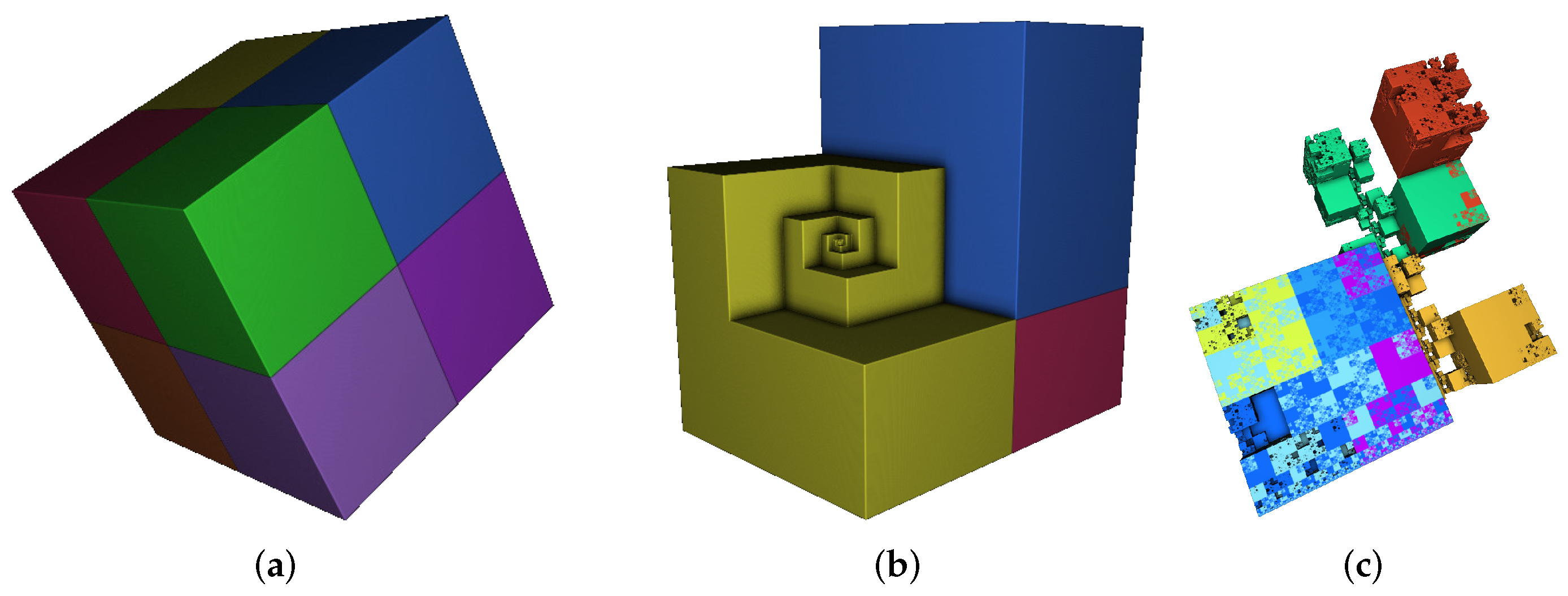
Unlike tilings of the plane ${\mathbb{R}}^2$, there are only few $m-$rep tiles known for $m<8$ in the 3-dimensional space. Even for $m=8$, not too many examples are known (see Figure 12 for some examples of polyhedral tiles). We refer to the papers [39,43,44] for important results and examples on the existence and non-existence of three-dimensional $m-$rep tiles and also to [45,46] for 3D tilings with large values of m. The rep tiles presented in these papers are produced using the similarity maps of the form $g\left(x\right)=mx$, and the IFS mappings have the form $f_j\left(x\right)=q_j\left(x\right)+r_j$ where $r_j$ denotes an integer translation and $q_j$ a symmetry map of the unit cube with center 0.

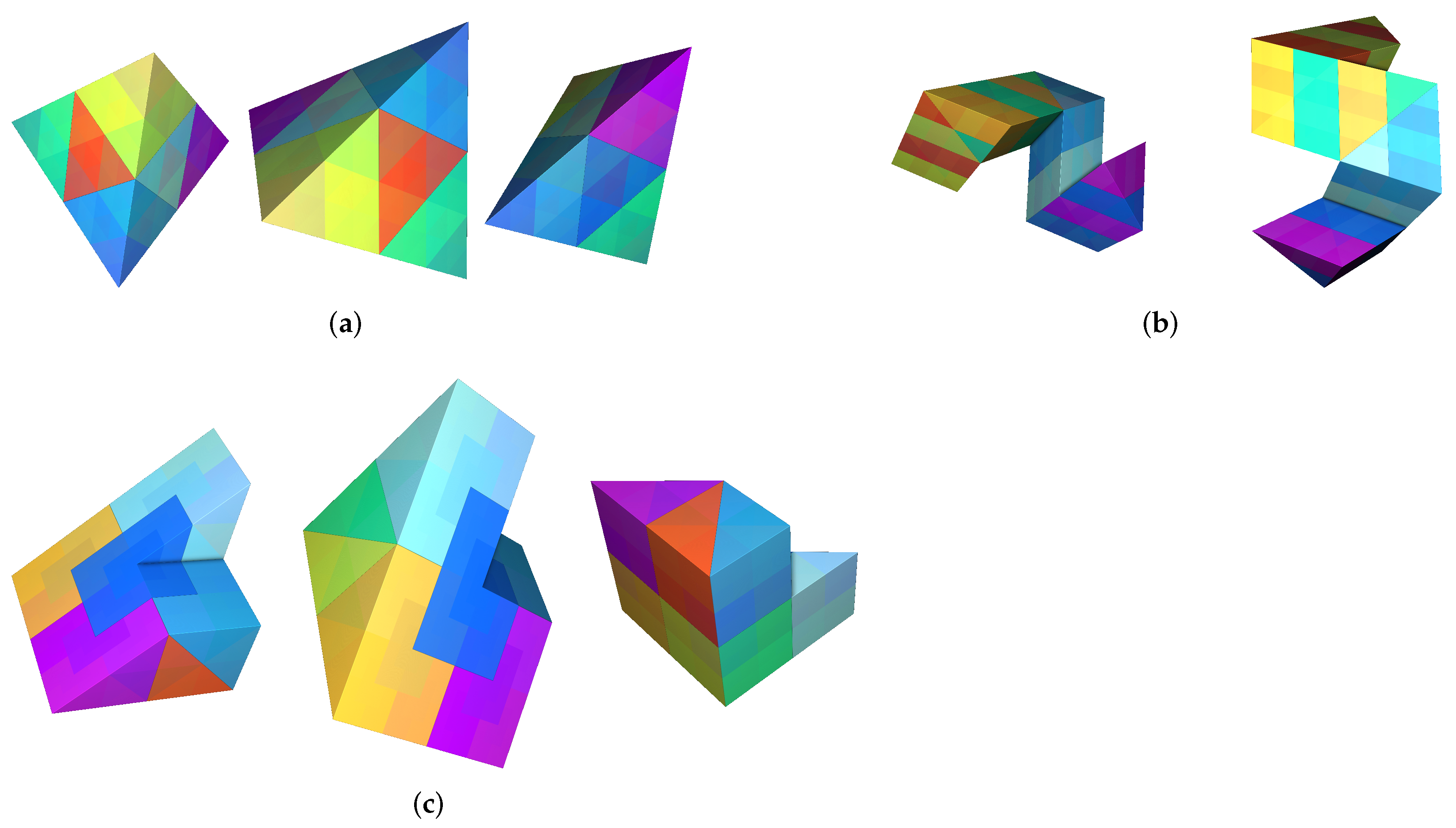
In three-dimensions, a tetrahedral $m-$rep tile can exist only for cubic numbers $m\ge 8$ [44]. For $m=8$, the cube is a standard rep tile, and the notched cube (‘chair’) tile in Figure 12 is another example. The regular tetrahedron or octahedron is not a $8-$rep tile. A special tetrahedra, which is an $8-$rep tile, was found by Hill in 1895 and the conjecture that there are no further $8-$rep tile tetrahedra [43,44] seems true till date.

Sometime ago, it was not known whether three dimensional $m-$rep tiles can have holes. In [45] an example with $m=24$ was given and in [46] a more sophisticated and interesting example with very large m is discussed. An interesting example of a new $8-$rep tile with a hole was found very recently by Bandt and Mekhontsev in [33] (see Figure 13).

A tile T is called a self-affine lattice tile if there is an affine expanding mapping g and a lattice L such that g preserves L and maps T to a union of tiles $T+k_i$ with $k_i\in L$. With respect to the standard basis vectors $e_i$, the map g has a matrix representation $g\left(x\right)=Mx$ where M is an integer matrix. We now state two important result of Bandt [39]. The first gives an algebraic criterion for a self-affine lattice tile and second implies that there are very few self-similar lattice tiles in ${\mathbb{R}}^3$.

A tile T is said to be conjugate to a self-similar tile if there is a linear map h so that $˜\tilde{T}=h\left(T\right)$ is a self-similar tile.

Proposition 1

(Proposition 2.2 [39]). A self-affine lattice tile with respect to $g\left(x\right)=Mx$ is conjugate to a self-similar tile if and only if all eigenvalues of M have the same modulus.

Theorem 5

(Theorem 2.3 [39]). If a self-affine lattice tile with respect to $g\left(x\right)=Mx$ in ${\mathbb{R}}^3$ is conjugate to a self-similar tile, then either $m=\left|det\right(M\left)\right|$ is a cubic number (in particular $m\ge 8$) or M is conjugate to the matrix $\left[\begin{array}{ccc}0& 0& \pm m\\ 1& 0& 0\\ 0& 1& 0\end{array}\right]$.

The geometries in 3D fractal tiles are caused by the self-affine fiber structure of the boundary, which makes the topology complicated. Apparently, the different eigenvalues of the generating matrix produce long and thin fibers, which can pierce the interior of neighboring tiles, or distort the boundary structure.

Bandt [39] developed algebraic tools which describe the geometry of a self-affine tile in arbitrary dimension, in a similar way as homotopy and homology groups describe the geometry of manifolds. The basic concept is the neighbor graph, which can be considered as a blueprint containing all information about the topology of a tile.

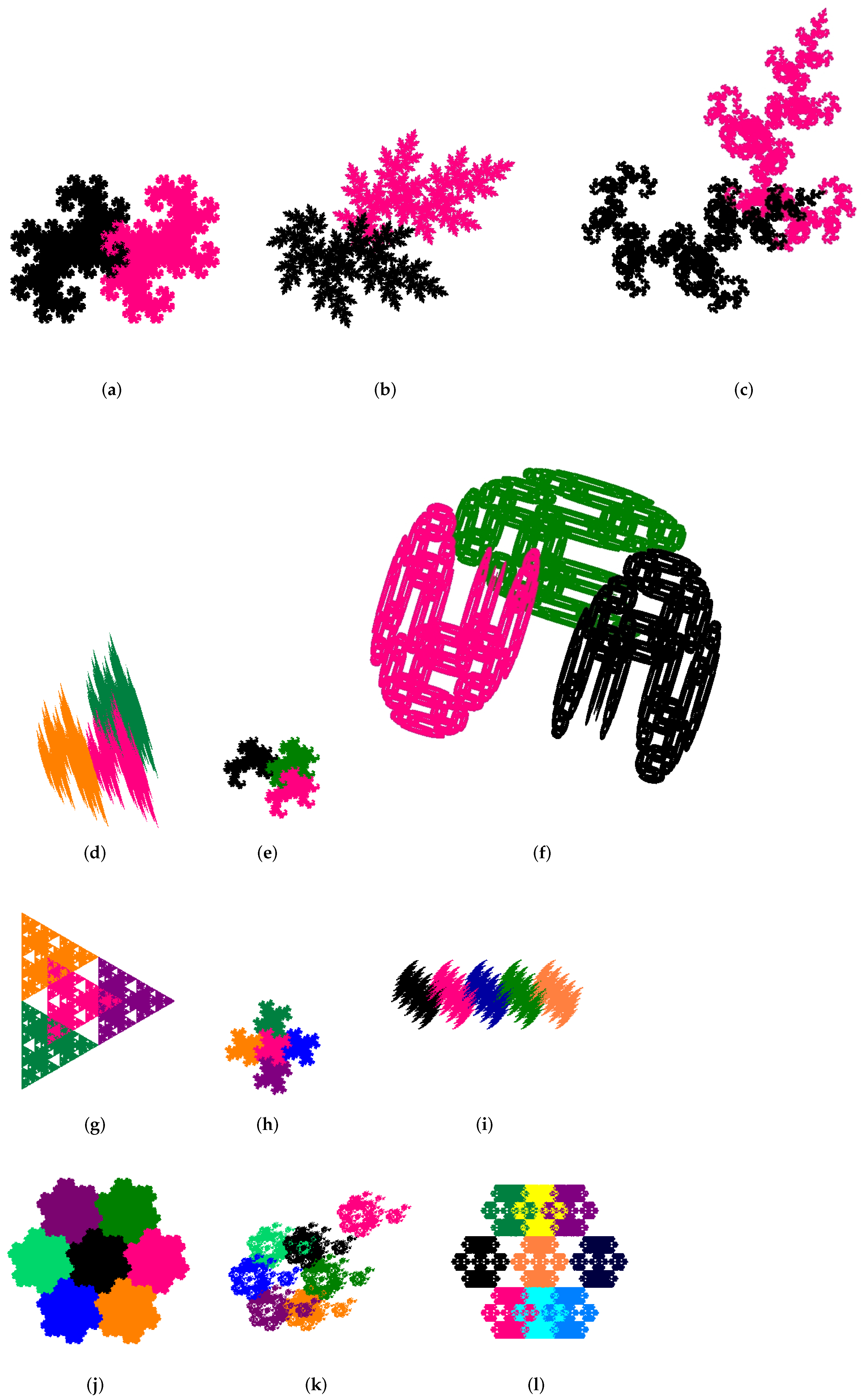
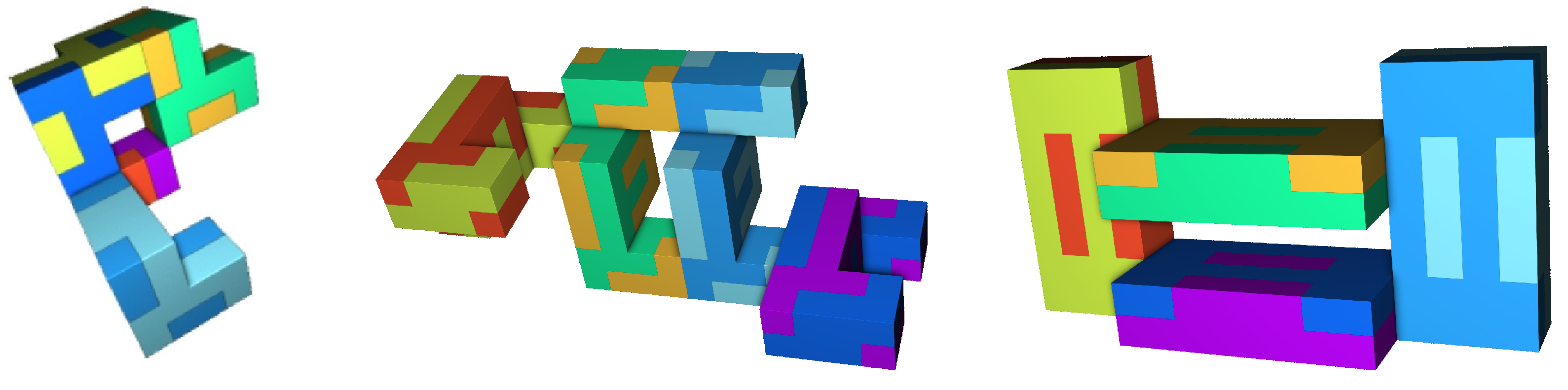
The recently developed software package IFSTile [41] is a good tool for computer-assisted mathematical analysis of three dimensional tilings and fractals. Figure 14 displays examples of non polycube $8-$rep tiles generated using IFSTile. the IFStile offers improved graphic and visualizations of fractal tilings with much greater functionalities. It can construct and search large families of self-similar tiles and fractals, and analyze them automatically in different ways. A lot of new examples with extraordinary properties can be found by the software. It can do rigorous and very fast calculations due to the use of integer arithmetics for rendering fractals. If the input data consist of real numbers then the package uses numerical approximation for rendering images. With IFStile package, structure and boundary of complex fractals and fractal rep tiles can now be computed within milliseconds specially in 3D case.

5. Fractals in Arts

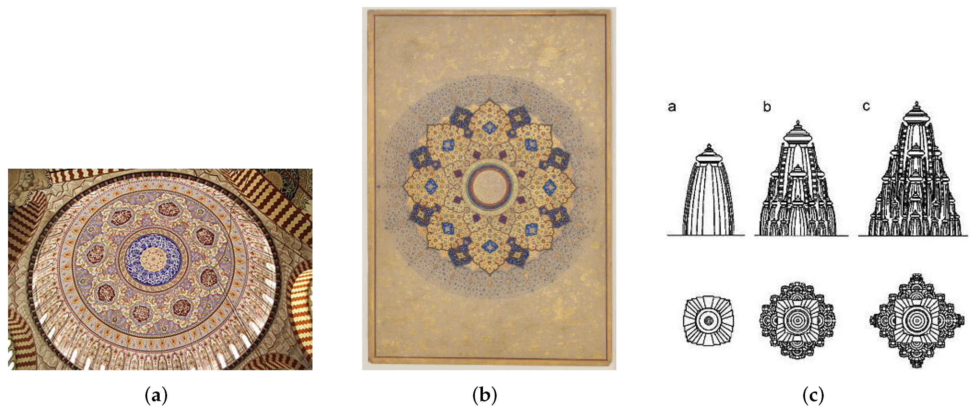
The mathematical beauty of fractals lies at the intersection of generative art and computer art. Fractal art is a genre of algorithmic art and digital art in which the results resemble the fractal objects or obey fractal properties. Fractal arts are also found in ancient times in manuscripts, hand-painted images, rugs, domes of mosques, and many more (see Figure 15 for some examples). Sculptures in temples built-in 15th–17th century have patterns which are reminiscent of fractal art so fractals were designed even before they were discovered. After the introduction of the Mandelbrot set in 1980s and the pioneering work by Mandelbrot in the classical book “The Fractal Geometry of Nature” [6], fractals have found applications in many areas and fractal arts is one of them.

Unlike other arts and paintings, the fractal arts are rarely designed by hands. They can be generated by many fractal generating computer software. Many artists modify the generated fractal images by adding non-fractal designs to make the image attractive. Though many new fractals are being discovered, yet Mandelbrot and Julia sets are considered as the benchmark icons in fractal art.

Fractals are generated by computer programs because of their complexity and numerous iterations to capture finer details. Popularity has been on the rise for fractal arts in the past few years. Many geometric patterns are being rapidly replaced by fractal arts, the prime reason being the aesthetic structure and self-similarity of fractals.

5.1. Fractal Art Galleries

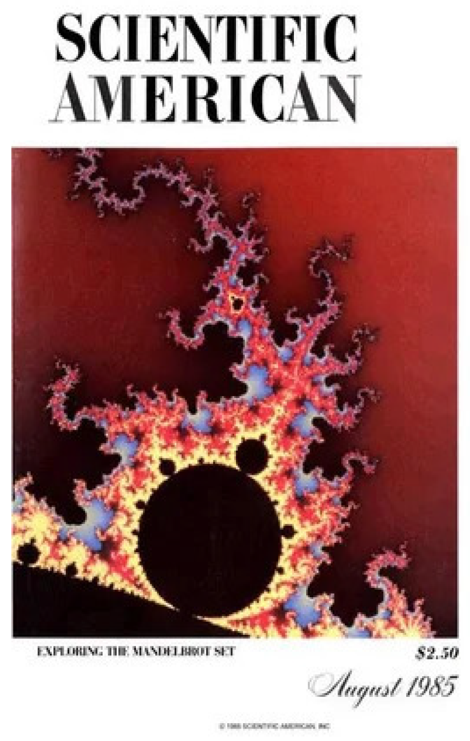
The first fractal image that appeared as an art work was probably on the cover page of Scientific American (August, 1985).

This image showed a landscape formed from the potential function on the domain outside the (usual) Mandelbrot set (see Figure 16); however, as the potential function grows fast near the boundary of the Mandelbrot set, it was necessary for the creator to let the landscape grow downwards, so that it looked as if the Mandelbrot set was a plateau atop a mountain with steep sides. The same technique was used a year after in some images in the book The Beauty of Fractals by Peitgen and Richter. They provided a formula to estimate the distance from a point outside the Mandelbrot set to the boundary of the Mandelbrot set (and a similar formula for the Julia sets). Landscapes can be formed from the distance function for a family of iterations of the form $z^2+a{z}^4+c$.

One of the first exhibitions to display fractal art was the “Map Art” (an exhibition of works from University of Bremen). Nowadays, fractal arts are being displayed in most of the international art galleries. Viewers of these galleries have showed interest in knowing the science behind fractals [47,48]. We also refer to the recent paper by Friedenberg et al. [49] for the aesthetic beauty and symmetry in exact and random fractals.

Artists generate fractal arts using fractal software which are processed further for enhancing the image quality and appearance. The fractal art images are usually printed using a DPI (Density Per Inch) ranging between 250–300 for capturing minute details of the image.

5.2. Fractal Art in Coloring Books

A coloring book is a book containing line arts that are intended to be filled with colors with no rules and regulations. The intention is to make them beautiful with their creative combinations of colors. Coloring books were introduced in 1880s by McLoughlin Brothers who also founded McLoughlin Bros. Inc., a New York based publishing firm and a pioneer in color printing technologies in children’s books. Figure 17 shows a few pages of the coloring book by Harrington [50].

Coloring books are used for many educational purposes, they are widely used in schooling for young children to enhance their fine motor skills and for improving their creativity level. These books are also used for studying graduate level anatomy topics for better visualization. Adult coloring books are different from children books and have intricate designs.

Designing complicated and detailed line art is not an easy task, however introduction of fractal art in coloring books made this easier. Since fractal arts are complex, heavily detailed and can be produced computationally with lesser human efforts therefore fractal art became a good fit into this field. In fractal coloring books the blank arts are the line arts of corresponding fractal arts. Fractal coloring books are very intuitively designed such that a blank line art is followed by colored image of that particular art and some details of the art are also mentioned so that a user can use them without difficulties.

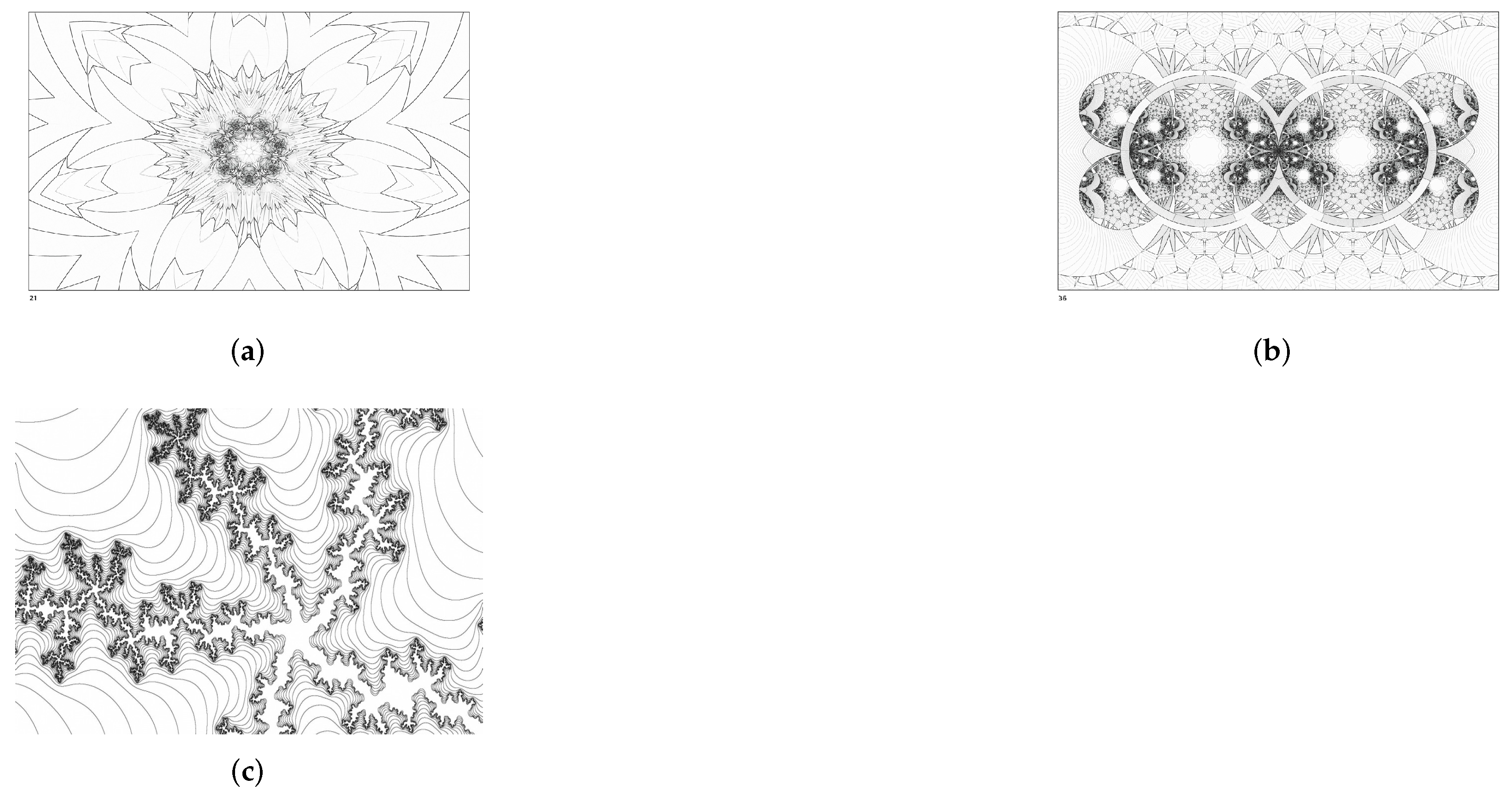
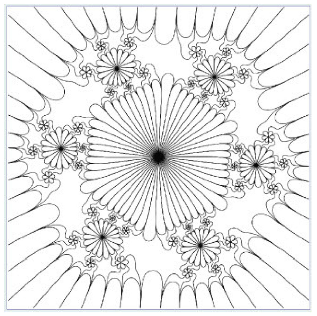
Figure 18 shows the shape of a complex-valued function from the coloring book by Barnes et al. [51]. It comes by composing the function

$$f\left(z\right)=z^3+\frac{-0.2+0.11i}{z^3}$$

with itself three times, computing the real part, and then plotting the level curves of heights 0, and 2. The book contains 18 such images and describes the mathematics in more detail.

5.3. Fractal Art in Ceramics

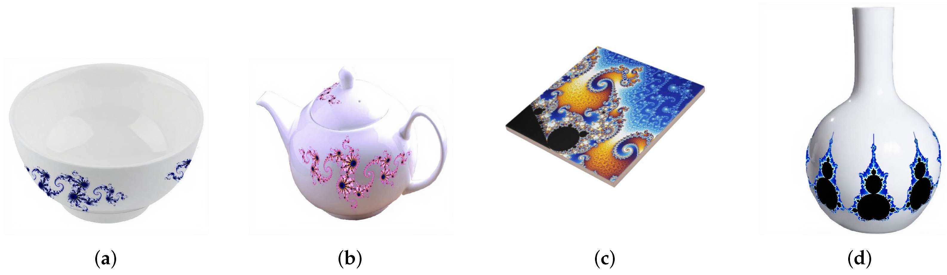
Ceramic products are widely used in our daily life. They serve us as teapots, tiles, bricks, flower vase, and many more. Painting these products with birds, flowers, and trees with landscapes make them attractive and provide customers a variety of choices.

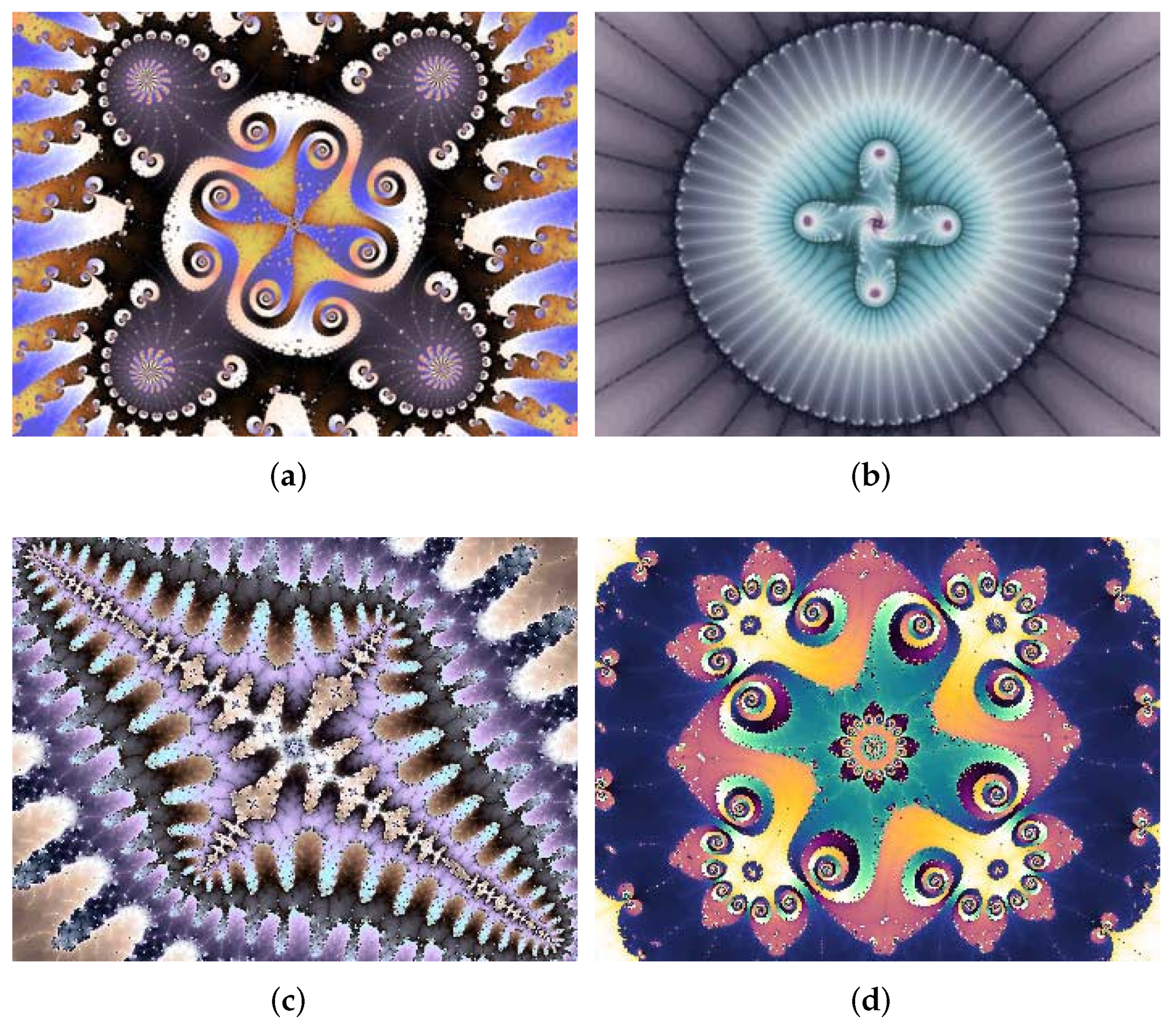
Fractals art can be used on ceramic products instead of the existing traditional designs owing to their aesthetic structures and symmetry properties.

These patterns convey a sense of natural beauty as many of the natural patterns are fractals and are different from traditional art. Fractal designs that are printed on ceramic products are selected very specifically depending on the utility of the product. For instance, the designs used on ceramic bowls are different from those of teapot designs since the environment and the frequency of usage of bowls is different from teapots (see Figure 19a,b). Similarly, flower vases are usually painted with fractals that are simple, symmetric, and resemble flower shapes (see Figure 19d).

Fractal arts are also used in painting tiles, which are now becoming popular. These fractal designed tiles are sold at much higher cost compared to the regular ones. Self-similar fractal patterns with vibrant colors and complex designs are preferred by buyers. Modern printing techniques help in printing the fractal designs on tiles with minute details to produce fractal designs at greater depths (see Figure 19c). The reader may refer to the papers by Lin [52] for applications of fractals in ceramic products.

5.4. Fractal Art in Screensavers

A screensaver is a computer program that blanks the screen or displays an image when computer is kept idle for a specified time. Originally, the screensavers were introduced to protect the monitor screens from burn-in (discoloration) and password protection. Typically, moving images, patterns, or animations are used as screensavers. Nowadays, the purpose of the modern screensavers has shifted to pleasure, entertainment, and advertisement rather than security and hardware protection. Microsoft introduced, Windows Spotlight in 2015 as a default screensaver in Windows 10 that displays beautiful pictures and advertisements from across the world with a customizable user interface.

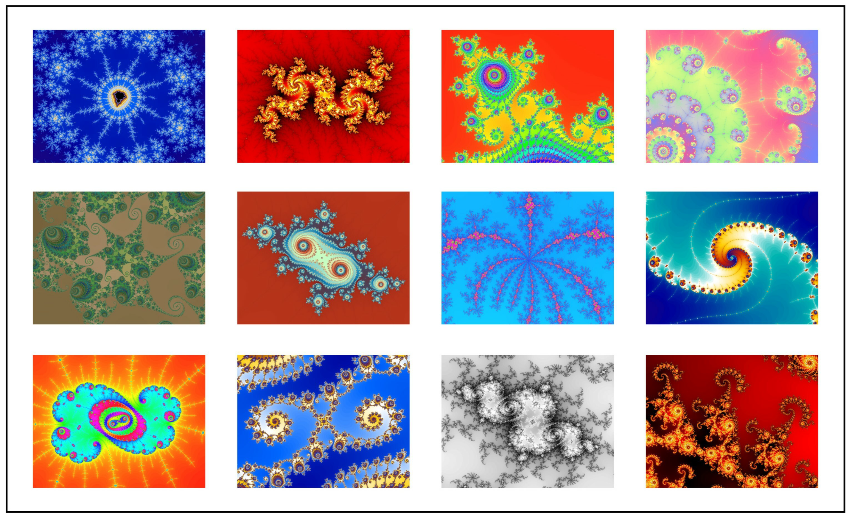
Use of fractal art in screensavers makes them more attractive, appealing and intense. Many still and animated fractal screensavers have been designed in which a particular fractal is formed and then explored or zoomed in for few seconds and then changes to new one or gets recycled as zooming deep requires higher computational powers. Figure 20 shows still images of an animated screensaver exploring the Mandelbrot set [53] and also look at Figure 21 for some examples of still screensavers.

Electric Sheep [54] is a distributed computing project for animating and evolving fractal flames, which are distributed to the networked computers, to display them as screen savers (see Figure 21d for an example of a fractal flame).

Fractal screensavers are one of the successful commercial applications of fractal arts. Heavy purchases are being made for fractal screensavers for commercial, personal use, and for gift purposes in today’s digital world.

5.5. Fractal Art in Calendars

“We made many pictures of it. The first one was very rough. But the very rough pictures were not the answer. Each rough picture asked a question. So we made another picture, another picture. And after a few weeks we had this very strong, overwhelming impression that this was a kind of big bear we had encountered!”

(B.B. Mandelbrot quoted about drawing Mandelbrot set by computers)

The Mandelbrot set is obtained by iterating the simple equation $f\left(z\right)=z^2+c$. The numbers in the Mandelbrot set equation are coordinates, defining the location of a point in the complex plane. When the Mandelbrot equation is given a number representing a point and that number is iterated through the equation then either the number becomes larger and bigger and escapes to infinity or it shrinks down to zero. Depending upon whatever is the case, the computer knows which point to plot and which point to leave. This iterative process yields a map, dividing this world into two distinct territories. Outside it are all the numbers that have the ‘freedom of infinity’. Inside it, numbers that are prisoners, ‘trapped and doomed to ultimate extinction’ yielding extraordinary, exciting, and infinite beauty of the Mandelbrot set.

Figure 22 shows a Mandelbrot calendar designed by David Eck, for January (top-left) through December (bottom-right) obtained by iterating the Mandelbrot set equation (for details, number of iterations, etc., the reader may refer to http://math.hws.edu/eck/mb21/, accessed on 20 October 2021).

5.6. Fractal Art in Exploring Infinity

The Mandelbrot set (see Figure 1) is the most famous fractal among all! Let us discover the infinite beauty of algebra by exploring the iconic Mandelbrot Set. There are several codes and software available to explore the details on the Mandelbrot set. We refer the reader to the Mandelbrot viewer [55] developed by David Eck for its simple interface and ease of use.

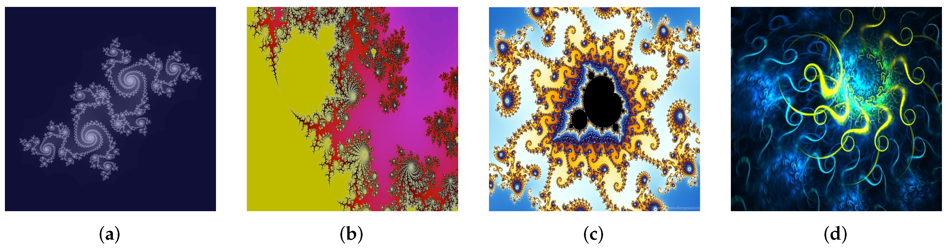
One of the most intriguing discoveries in the Mandelbrot set is that as you zoom into it, you will find an infinite number of tiny copies of the entire object and countless examples of self-similar patterns. No matter how much you magnify the set, a million times, a billion times (until the original set is bigger than the entire Universe!), you would still see new patterns, new images emerging. You will see shapes that resemble a cat, a cactus, a cockroach, elephant trunks, tentacles of octopus, sea horses, compound insect eyes, and so on. It shows us almost anything that we can see in the real world, particularly living things. There is indeed an infinite variety present in the Mandelbrot set just as is in nature.

Interestingly, unlike the self-similar IFS fractals, which show the same kind of details at all scales, the Mandelbrot set is not perfectly self-similar. The shapes of the objects from different parts of this fractal are dramatically different. Furthermore, the patterns can gain in complexity and beauty the deeper you explore and each of these replicas is as complicated as the original, and you could explore the details around the edge of a replica as well; of course, you can find even smaller replicas, around the replicas, and so on.

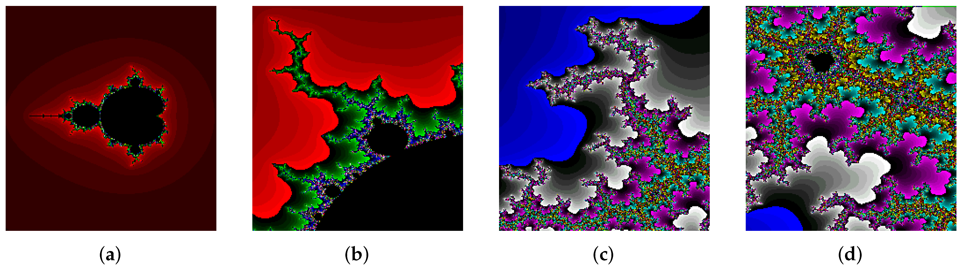
The four images in Figure 23 are all inconceivably tiny details from different areas deep within the Mandelbrot set with a magnification depth range of ${10}^{74}$–${10}^{245}$, and are far smaller than anything in the real universe and they are all connected!

Let us try to imagine the sizes of these mathematical objects. A reasonable estimate for the size of the universe is 100 billion light years, or roughly ${10}^{27}$ meters. At the other end of the range, the smallest theoretical scale (known as the Planck Length) is approximately ${10}^{-35}$ meters; therefore, the entire range of scale from the smallest to the largest in our universe is 27 − (−35) = 62 orders of magnitude. Clearly, the range of scale between the whole Mandelbrot set and the zoomed-in detail in Figure 23a (at the top right), which is magnified ${10}^{74}$ times, is ${10}^{12}$, or a trillion times bigger than the whole scale of our universe. Yet these incredibly tiny images are just a scratch on the surface of the infinite Mandelbrot set!

6. Fractals in Fashion Designing

Clothing coexists from the very beginning of human evolution and it is considered as one of the factors for human survival. Clothing styles have evolved with improvement in technology and available resources. People have shifted to textiles and have been using particular fabrics for particular purposes based on some factors such as occasion, locality, weather conditions, etc. Clothing has a huge demand in the market, which resulted in many fashion brands emerging in this field. The introduction of fractals in art grabbed the attention of researchers with its features that have never been seen before such as self-similarity, symmetry, pattern regularity, etc., and artists started using fractal art in cloth designing.

Textile designs are very important in the art world. The designs and fabrications have changed from culture to culture, artist to artist, expressing history and experiences throughout generations. With the development of algorithms and software for rendering fractals, fractal-designed textiles are expected to play a key role for new innovations and ideas in the field of design. Applications of fractals in compressing images by reducing data redundancies is a perfect platform for textile design (see Section 6). Among many algorithms for generating fractals, $L-$system generation algorithm and Julia set generation algorithms are primarily used for fractal garment pattern generation and textile designs.

Jhane Barnes, a well known textile artist, redefined fashion textiles using weaving and textile software. Her creative computer-generated fractal designs revolutionizing the world of textile designs. These fabricated textiles are created for men’s wear, women’s wear, carpet designs, and home decor. She was featured in a chapter of McDougal Littell’s textbook entitled ‘Sequences and Series: Fractals for fashions’.

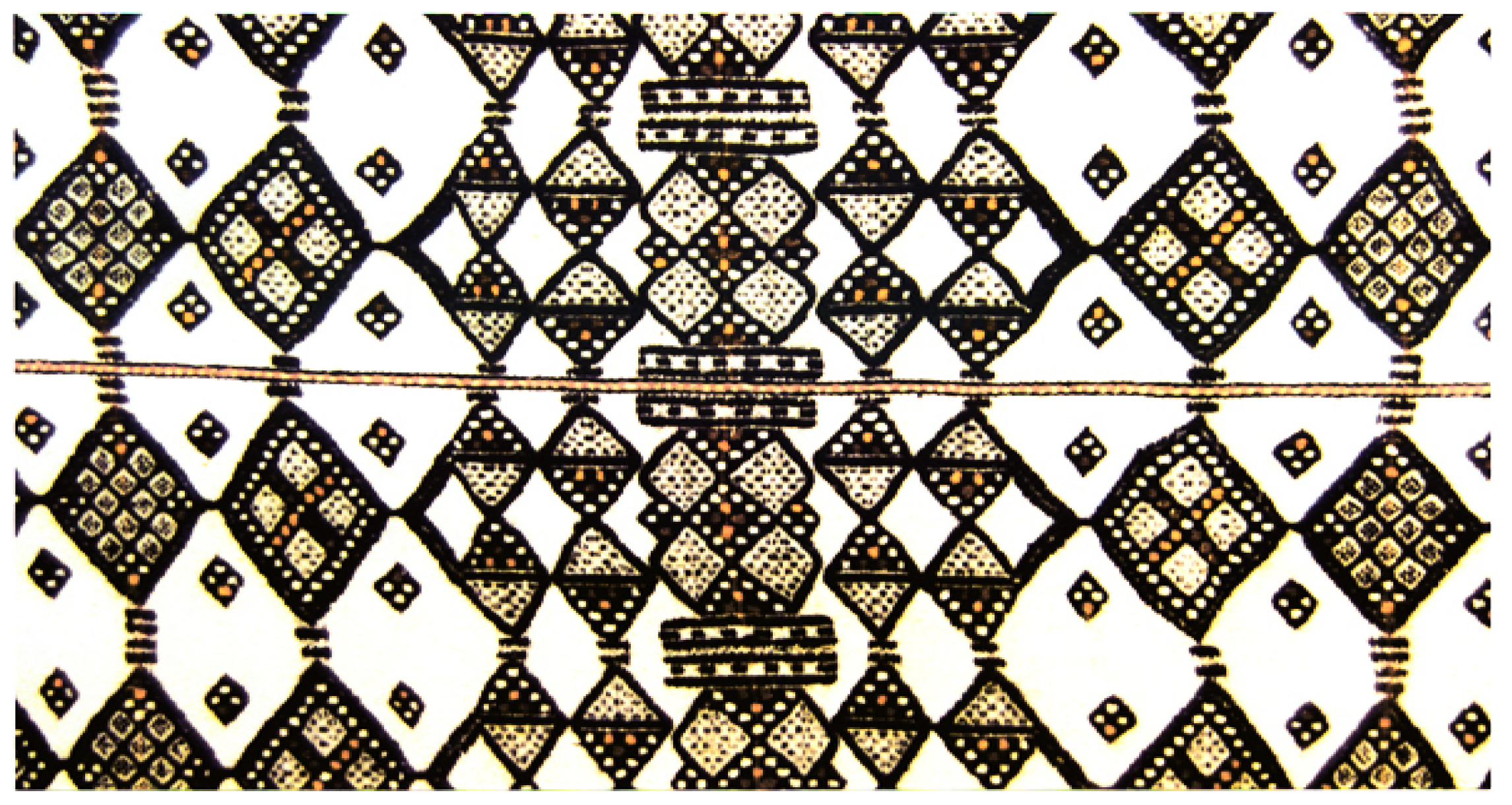
Figure 24 shows the iterative construction of a Fulani wedding blanket on the cover page of the book entitled “African Fractals: Modern Computing and Indigenous Design” by Dr. Ron Eglash (see Available from https://roneglash.org/eglash.dir/afractal/afbook.htm for more, accessed on 20 October 2021). The diamonds in the blanket become smaller as you move from either side towards the blanket’s center. Eglash wrote “The weavers who created it report that spiritual energy is woven into the pattern and that each successive iteration shows an increase in this energy”.

Geometrical design and flower design are common themes in clothing design. We briefly present standard fractal garment pattern generation algorithms along with examples and refer the reader to the recent work by Wang et al. [56] for a detailed journey through applications of fractals into garment designs.

6.1. $L-$System Garment Pattern Generation Algorithm

The $L-$system pattern generation method was first introduced as a method to describe plant morphology and growth process by Danish biologist Aristid Linden-Mayer in 1968 [57], which later developed into a method to simulate natural scenery in computer graphics. The working of the $L-$system is simple, it can be operated with very few characters whose function is predefined. The core idea of an $L-$system is string replacement where a string pattern is generated, which is expected as output and then the string is iterated through simple transformations and is converted into a long string generating a fractal art. In practice, the iteration number is usually kept in the range of 3 to 10.

The string of an $L-$system is also called turtle graph. A state of turtle is defined as $(x,y,\alpha )$ where $(x,y)$ is the position of the turtle in the $xy-$plane and $\alpha$ is the direction that the turtle face is facing.

The string generated after applying transformations to an initial string turns out to be a fractal. The parameters such as axiom (initial element), production formula (generator element), compression factor, iteration number, and angle increment $\delta$ are set by the designer as per requirement. We illustrate the fractal pattern generation using $L-$system with an example [56].

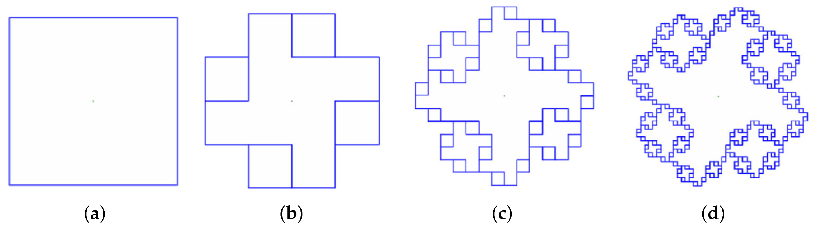
Example 6.

Assume that the initial angle is $0^{\circ }$, angle increment $\delta ={90}^{\circ }$, axiom $w:f+f+f+f$, generating formula $p:f\to ff-f-f-f-f+f$, and the compression factor is $\frac{1}{3}$. Here, f means move the turtle forward one step along a straight line. This will change the state of the turtle from $(x,y,\alpha )$ to $(x^{\prime },y^{\prime },\alpha )$, where $x^{\prime }=x+\delta ·cos\alpha$, $y^{\prime }=y+\delta ·sin\alpha$, ($\delta =$angle increment in α). + means, rotate the turtle by angle δ in counterclockwise direction. By this command, the turtle’s state will change from $(x,y,\alpha )$ to $(x,y,\alpha +\delta )$ and − means, rotate the turtle by angle δ clockwise. This will change turtle state from $(x,y,\alpha )$ to $(x,y,\alpha -\delta )$.

The initial element is shown in Figure 25a and Figure 25b–d are generated with the number of iterations $n=1,2$, and 3, respectively.

The patterns generated by $L-$system are linear and the graph generated by the $L-$system can not only simulate the growth of flowers, plants, and trees, but it can also generate various geometric figures with fine structures. Combining with computer graphics technology, a series of geometric patterns can be designed. $L-$system codes are written in many latest technologies such as MATLAB, Python, etc., to generate these patterns. For the flow chart of the $L-$system pattern generation we refer the reader to [56].

6.2. Garment Pattern Generation through Complex Dynamical System (Julia Sets)

The computer aided pattern technology combined with complex dynamical system theory can be used to generate fractal art graphics. Designing patterns via complex dynamical systems is indeed the process of generating Julia sets using the escape-time algorithm.

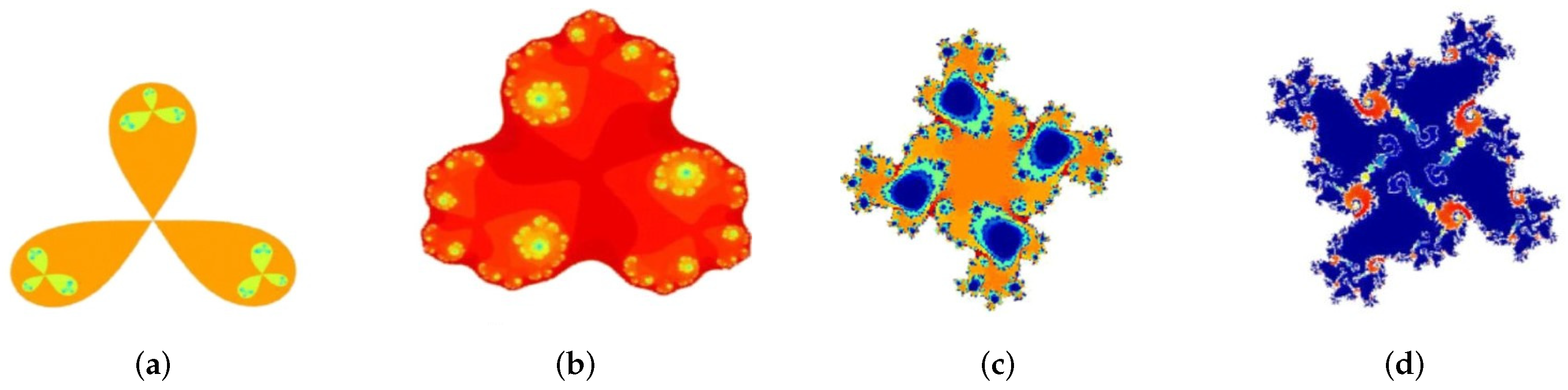
Julia sets are generated using escape time algorithm by iterating the equation $z=z^n+c$ and the shape of the generated Julia sets can be controlled using the parameters c and n. The triangular and the quadruple pattern are two common types of garment patterns, which are generated using the Julia set pattern generation method. Figure 26a,b displays two triangular patterns generated using the Julia set pattern algorithm with the function $z=z^3+c$. Figure 26c,d shows two Quadruple four-corner patterns designed using Julia’s plot program. In these patterns the value of n is either 4 or 6. The value of the parameter c is indicated below each pattern.

A few basic patterns can be integrated together to amplify the beauty of the pattern. Two such examples are shown in Figure 27. Figure 27a shows a garment pattern, which is a combination of basic patterns generated by $L-$system and Figure 27b displays another pattern formed by combination of basic patterns from Julia set algorithm.

After integrating these two patterns, the pattern as a whole is also considered as a basic pattern (see Figure 27c). While designing a garment, a pattern is limited to a particular size and then repeatedly filled throughout the garment in different orientations based on beauty principles of clothing designs. The new basic pattern in Figure 27c is used for filling particular dimensions of the fabric as shown in Figure 27d.

6.3. Fractal Designs on Silk Scarves and Garments

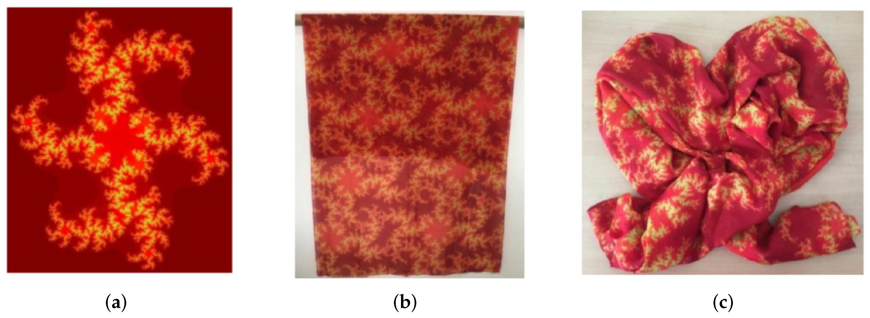
Silk scarves are important clothing accessories, which are equipped with unique cultural characteristics, influenced by aesthetic taste and customs and the patterns on the silk scarves are the soul of scarves. The traditional silk scarves designs consist of patterns based on natural elements such as flowers, plants, sceneries (landscapes), etc. Fractal based designs for silk scarves are motivated by the intrinsic self-similarity and symmetry present in fractals, which provides a stable and official look to the designs.

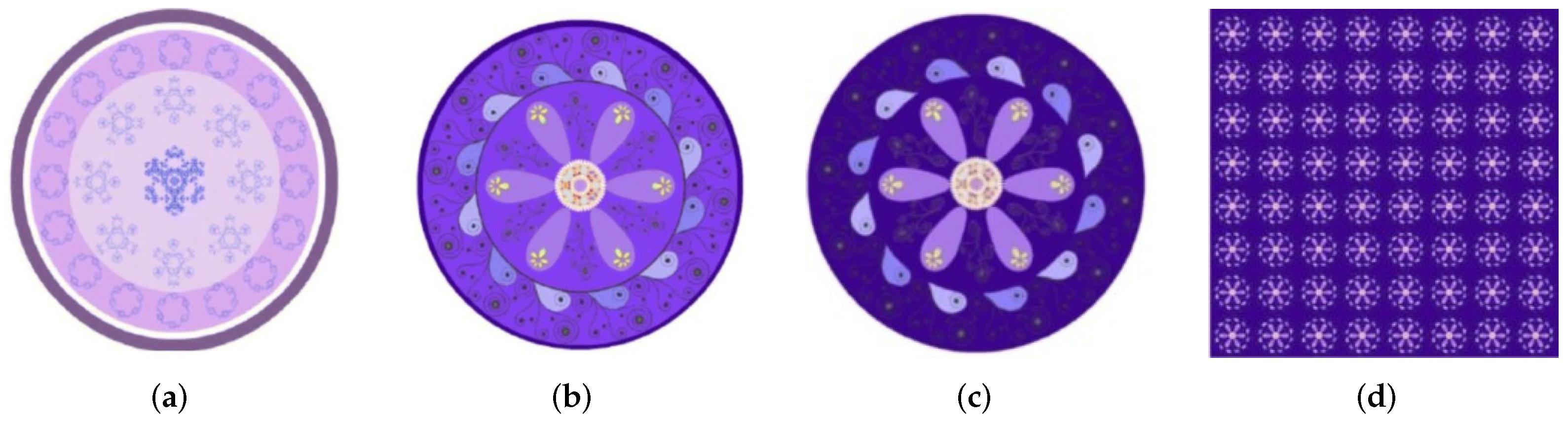
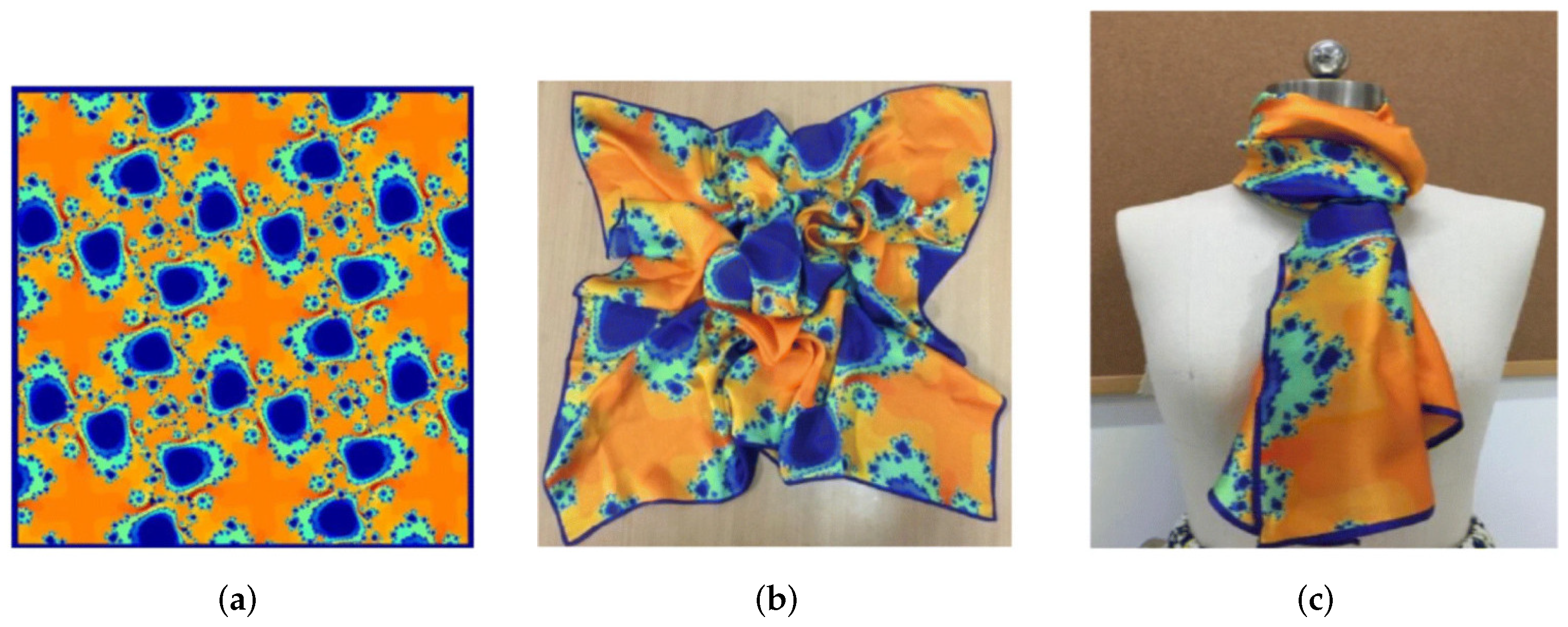
A computer generated square shaped silk scarf is presented in Figure 28 using the basic pattern diagram from the Julia set in Figure 27c. The individual patterns are arranged as scattered squares to obtain the silk scarf pattern (see Figure 28a). The contrast and suitable color configuration produces strong, lively, bright, and eye-catching feeling.

Finally, the silk scarf pattern is made through digital printing, and the real object diagram and the wearing effect diagram are obtained, which are shown in Figure 28b,c, respectively. Figure 29a shows another basic pattern for fabric design generated from the Julia set algorithm. The fabric pattern is digitally printed in Figure 29b,c, which is obtained through continuous arrangement of the basic pattern.

6.4. Summary

Fractal garment patterns can be generated using computer assisted pattern technology combined with the dynamical system theory by changing parameters in the escape time algorithm and using $L-$systems. As a new design resource, fractal clothing is attracting attention in the field of design. The fractal pattern generation theory can be applied to construct appealing designs for garments, scarves, T-shirts, and other fashion costumes. We refer to the papers [58,59,60,61] for further reading into fractal garment pattern designs and their applications in fashion.

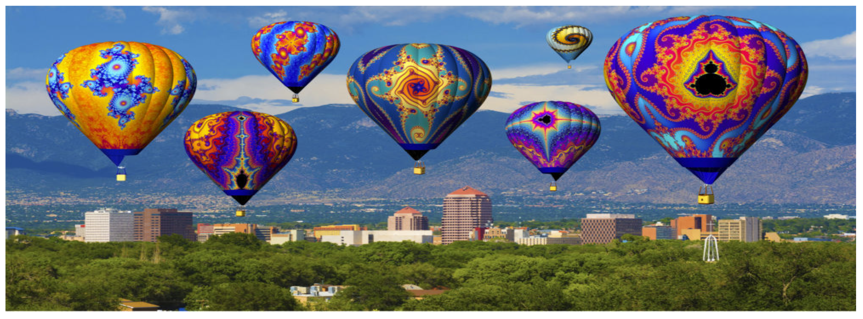
7. Fractals in Hot Air Balloons

The Fractal Foundation [62] announced the first ever digitally printed flying fractals in the form of fractal art balloons in 2018. These are the first ever balloons of their kind, fully digitally printed (using advanced dye sublimation printing technology) mathematical artworks. The images on the balloons are tiny details of the Mandelbrot Set, magnified billions of times.

The fractal images consist of hundreds of billions of pixels, which can be seen from either millimeters or miles away! They are manufactured by Kubicek Balloons in the Czech Republic, and are approved by the FAA as standard certified aircraft (see Figure 30).

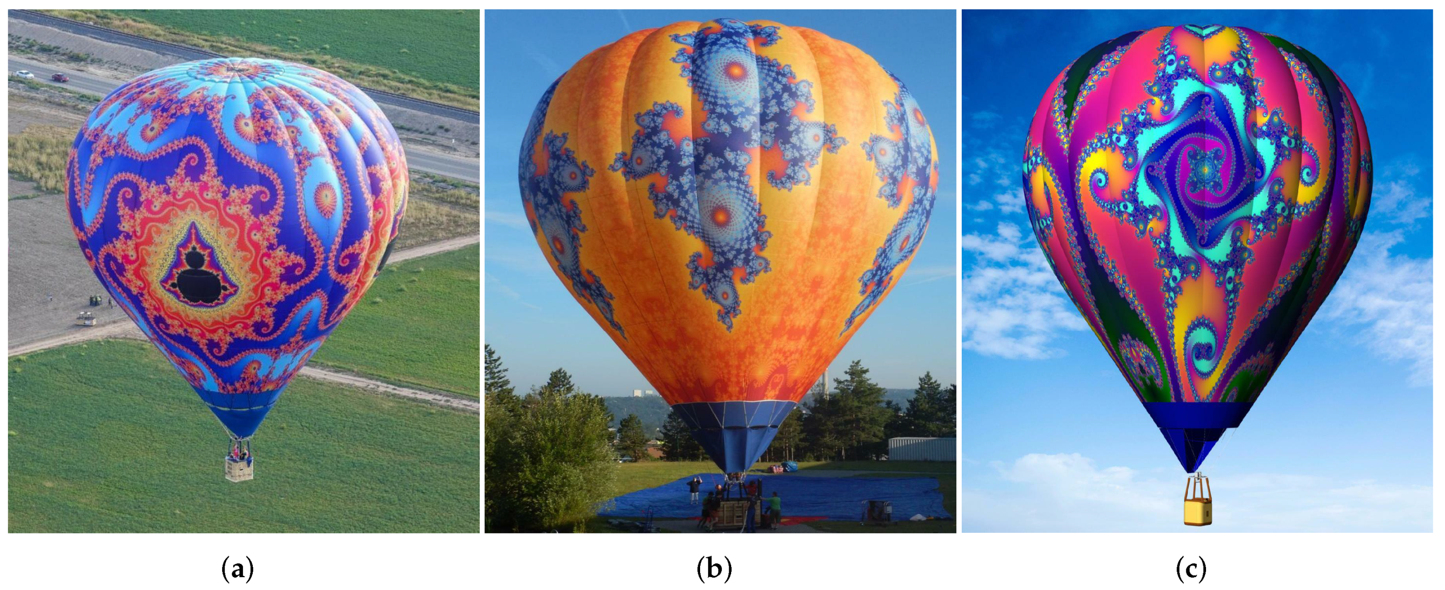
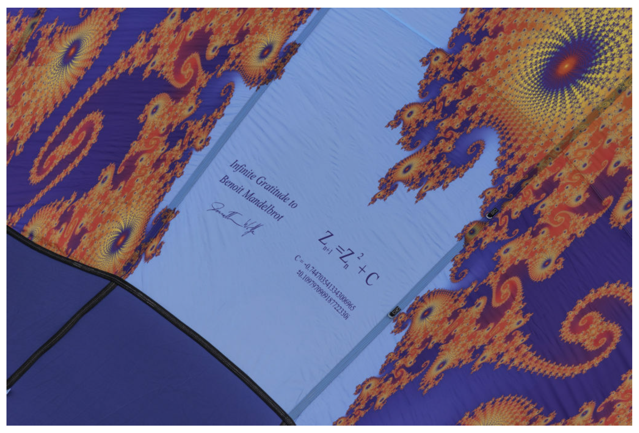
“Infinitude” (Figure 31a) is based in Albuquerque, New Mexico, and “Fibonacci” (Figure 31b) is based in Pennsylvania. Both balloons bring lots of inspiration among audiences towards the beauty of math and science. A dedication to Mandelbrot, the formula $f\left(z\right)=z^2+c$, and the coordinates that generate the image are shown at the mouth of “Infinitude” balloon. The dedication reads “Infinite Gratitude to Benoît Mandelbrot”. “Infinite Gratitude” was then renamed to “Infinitude”—which became the name of the balloon (see Figure 32).

The fractal is zoomed in 7 billion times from the original Mandelbrot set. The entire image contains over 100 billion pixels, making it one of the highest resolution fractals ever made.

“Fibonacci” was named in honor of “Leonardo Bonacci” (13th century Italian mathematician) who first brought the Hindu–Arabic numeral system to Europe, including the concept of Zero, which makes modern arithmetic and algebra possible. The famous Fibonacci sequence approaches the golden ratio $\Phi =\frac{1+\sqrt{5}}{2}$, and is found in many natural fractal patterns (e.g., sunflowers) and which is reflected in the central design motif of the balloon. “Fibonacci” in Figure 31b is the largest, highest resolution fractal ever printed, which contains over 340 BILLION pixels! An unnamed future balloon is shown in Figure 31c.

8. Fractals in Econophysics

The term econophysics was coined by the scientist H. Eugene Stanley from Boston University (H.E. Stanley [63]). Econophysics is a newly developing field of research, which is based on probabilistic and statistical physics to understand and solve economic problems in stock and other markets, especially those with uncertainties, stochastic processes, and non-linear dynamics. The first econophysics work that gained huge popularity was the paper by Mantegna and Stanley [64], which essentially developed the idea of Benoît Mandelbrot concerning the Lévy flight [65]. Ever since, experts are familiar with the proposition that movements of prices of most financial markets over time and price scales look self-similar. An observer cannot identify from the shape of the charts if the data describe weekly, daily, or hourly fluctuations. In the modern terminology of today, the indicated self-similarity signifies that financial time series are fractals. Fractal dimension (D), Hurst exponent (H), and sample entropy (S) are the parameters that help to analyze the complexity of the time–series signals arising in financial markets. The Hurst exponent (or more appropriately, the self-similarity index) is used to analyze self-similarity patterns for financial time series. It allows researchers exploring memory in cryptocurrencies, identifying bubbles, and even forecasting the behavior of markets, to name a few. For a self-similar time series, the Hurst exponent H, which is a measure of persistence (long-term memory) of a time series is related to the fractal dimension by the relation $D=2-H,1<D<2$, [66]. The Hurst exponent vary between 0 and 1, with higher values indicating a smoother trend, less volatility, and less roughness. For more general time series or multi-dimensional processes, the Hurst exponent and fractal dimension can be chosen independently, as the Hurst exponent represents structure over asymptotically longer periods, while fractal dimension represents structure over asymptotically shorter periods [67]. Similar to fractal dimension, sample entropy is also a measure of complexity and it is related to the Hurst exponent via two parameters namely the tolerance r and embedding dimension m, which control, respectively, the level of similarity between samples (data points) and the length of each template within a sample.

The book by M. Fernández-Martínez et al. [16] provides a novel and robust theory of fractal dimension for fractal structures with applications to artificial intelligence, and econophysics. The book contains new algorithms to calculate the Hurst exponent of (financial) time series. By means of several theoretical results it is shown that the Hurst exponent is related to a new fractal dimension for curves that count for fractal patterns in the image set of a curve (resp., a time series) instead of the graph of the curve. The review paper [68] summarizes the financial models of econophysics arising from fractal market analysis that are primarily based on the Hurst exponent and highlights some of the empirical applications within the study of the financial market. For further reading on fractal analysis of time series in econophysics using fractal dimension and Hurst exponent we refer to [69,70].

9. Fractals in Military Applications

Antenna is a main contributing source to the overall radar cross-section (RCS) in military purposes. The RCS reduction is crucial for aircraft, missiles, ships, and other military vehicles because military vehicles with smaller RCS can evade easy radar detection, whether it be from land-based installations, guided weapons, or other vehicles. The development of fractal shaped antenna arrays with miniaturization, ultra-wideband (UWB), high-gain, and low-scattering characteristics have attracted increasing attention in recent years in modern communications systems for military applications. These fractal shaped, small size antennas can operate at multiple frequencies for small satellite communication terminals, and other wireless applications for use by military. Fractal antenna’s compact design provides superior wideband performance and being compact they can be mounted or embedded in a variety of locations without conveying their frequency range. Fractal antennas can be used for vehicle, marine, airborne, fixed, or personnel-worn applications. With extreme wideband frequency range, fractal antennas are uniquely suited to enable leading performance and interoperability between legacy and new radio architectures. A primary example is the MHA, a wideband colinear antenna developed by Fractal Antenna Systems with excellent gain and omnidirectional pattern over the UHF and microwave range, all in an antenna that is only 42 inches long. A microstrip hexagonal fractal antenna for military applications was proposed in [71]. For a brief introduction to fractal antennas we refer to the Section 18.4 of Falconer’s book [8].

Fractals are also being used by some armies (e.g., German military troops) to design their camouflage clothes and equipment. How to generate fractals for such purposes and what are the advantages of using fractals in this regard are some of the questions that are still in developmental stages.

10. Book Recommendations and Fractal Generating Software

Plenty of textbooks and monographs are available on fractals and their applications and we provide a few for further reading. The classical books of Mandelbrot [3,6,19] contain a great deal of information and basics about fractals. The monograph [2] is a collection of articles by researchers and collaborators of Mandelbrot. For graduate level courses in deterministic fractal geometry and its mathematical foundations we refer to the popular books by Barnsley [5], Falconer [8], Peitgen et al. [72], and Edgar [13]. The book by Gulick [73] focuses on chaos and fractals and diverse applications of chaotic dynamics and fractal geometry within mathematics and in many other disciplines. For concepts and applications of fractals in geosciences, we refer to [74]. A beautiful collection of computer generated fractals can be found in [75] with a link to the software for the images, and for further exploration. For a unified list of almost all the works on fractal geometry by Mandelbrot and other researchers we refer to [4].

There are several computer software and resources that are available for for rendering fractals and tilings. Fractint is one of the oldest fractal program written in DOS format, which was later updated to Winfract. Other advanced fractal rendering software include IFSTile, IFS Builder 3D, IFS Construction Kit, Fractracer, Chaoscope, Ultra Fractal, Fractal Explorer, Mandelbulb 3D (MB3D), FractalWorks, FracLac, etc. For creating interactive, real time zoom on fractals, we refer to XaoS. Most of these software use the random iteration and deterministic algorithm to generate beautiful, symmetric fractals.

11. Conclusions

An eclectic survey encompassing the mathematics and characterization of fractals (using IFS, attractors, fractal dimension, etc.), along with applications in a number of exciting fields including emerging ones has been presented. The article explores both natural and manufactured fractals from mathematical and technical aspects. Aesthetic and artistic beauty of fractals is further investigated into arts, fashion designing, and in tessellations.

In the forthcoming second part of this survey, we shall consider engineering, industrial, and commercial applications of fractals in many fields ranging from fractal landscape generation, design of fractal shaped antennas, fractal image compression, fracture mechanics, and some future applications as well.

Describing fractal geometry in the classic book “Fractals Everywhere”, Michael Barnsley wrote, “Fractal geometry will make you see everything differently. There is a danger in reading further. You risk loss of your childhood vision of clouds, forests, galaxies, leaves, feathers, flowers, rocks, mountains, torrents of water, carpets, bricks, and much else besides”.