Abstract
In this article, we develop a numerical method based on the operational matrices of shifted Vieta–Lucas polynomials (VLPs) for solving Caputo fractional-order differential equations (FDEs). We derive a new operational matrix of the fractional-order derivatives in the Caputo sense, which is then used with spectral tau and spectral collocation methods to reduce the FDEs to a system of algebraic equations. Several numerical examples are given to show the accuracy of this method. These examples show that the obtained results have good agreement with the analytical solutions in both linear and non-linear FDEs. In addition to this, the numerical results obtained by using our method are compared with the numerical results obtained otherwise in the literature.
1. Introduction
Fractional calculus has been playing a very important role in scientific computations. Scientists are able to describe and model many physical phenomena with fractional-order differential equations. As a result, fractional-order differential operators are widely used to solve systems by developing more accurate models [1,2,3,4]. The nonlocal property of the fractional-order operators makes them more efficient for modeling the various problems of physics, fluid dynamics and their related disciplines [1,5,6,7,8,9]. For example, consider a thin rigid plate of mass and area R immersed in a Newtonian fluid of infinite extent and connected by a massless spring of stiffness K to a fixed point. A force is applied to the plate. Assume that the spring has no effect on the fluid and that the area of the plate is large enough to produce the fluid adjacent to the plate, whereas stresses can be defined by the following relation:
where x is the distance of a point in the fluid from the spring to the submerged plate. By some assumptions discussed in [10], the dynamics of the system are given by
where . Equation (2), with some assumptions considered in [10], takes the following form of a Bagley–Torvik-type problem solved in (Section 6, Example 1):
The existence and uniqueness results of fractional-order differential equations (FDEs) have been investigated extensively in the literature. Some of them are presented as follows: Fazli and Nieto [11] investigated the existence and uniqueness of the solution of FDEs of Bagley–Torvik type by considering the existence of coupled lower and upper solutions. Pang et al. [12] investigated the existence and uniqueness of the solution of the generalized FDEs with initial conditions by proposing a novel max-metric containing a Caputo derivative. Abbas [13] studied the existence and uniqueness of the solution of FDEs by using Banach’s contraction principle together with Krasnoselskii fixed point theorem. For more works on existence and uniqueness results, we refer the reader to [14,15,16,17].
As most FDEs do not have closed-form solutions, different numerical techniques, including the finite difference method, variational iteration method and spectral methods, are preferably used. Among them, spectral methods have received considerable attention from the fractional community for solving FDEs, both ordinary and partial. Spectral methods are classified into three types, known as the collocation, tau and Galerkin methods. The basic idea of the spectral methods is to write the solution as a linear combination of basis vectors of global polynomials, typically Legendre, Jacobi and Chebyshev. The speed of convergence is considered the best advantage of the spectral methods, as the rate of convergence is exponential in these methods, which gives a high level of accuracy. Many efficient spectral techniques are obtained in the literature using the various global polynomials [18,19,20,21].
The construction of the operational matrices of fractional derivative operators defined with singular or nonsingular kernels has played a key role in the development of spectral methods. Many researchers have worked on the construction of the operational matrices of fractional derivatives using different types of global polynomials. For example, Benattia et al. [22] introduced the operational matrix of the fractional derivatives to develop a numerical method that is based on the Chebyshev wavelet for solving FDEs. Saadatmandi et al. [23] derived an operational matrix of derivatives of fractional order using the fractional-order Chebyshev functions. They also extended the results of [23] for solving the coupled system of FDEs with variable coefficients [24]. Additionally, Bharway et al. [25] introduced a new shifted Chebyshev operational matrix of fractional integration for solving linear FDEs. Moreover, Talib et al. [26] developed a new operational matrix based on the orthogonal shifted Legendre polynomials to numerically solve the fractional partial differential equations. Meanwhile, Rahimkhani et al. [27] introduced a Bernoulli wavelet operational matrix of fractional integration for obtaining the approximate solution of a fractional delay differential equation. Kazem et al. [18] derived an operational matrix that generalized the results presented in [19]. Recently, Dehastani et al. [28] calculated modified operational matrices of integration and pseudo-operational of fractional derivatives for the Lucas wavelet functions to compute the numerical solution of fractional Fredholm–Volterra integro-differential equations. Moreover, Dehastani et al. [29,30] also derived operational matrices of fractional-order derivatives and integration for fractional-order Bessel functions and fractional-order hybrid Bessel functions. In the derived numerical techniques, the operational matrices are applied to reduce the FDEs to a system of algebraic equations.
Dehestani et al. [31] also presented a novel collocation method based on the Genocchi wavelet for the numerical solution of FDEs and time-fractional partial differential equations with delay.
Motivated by the aforementioned works, we extend the study of the spectral methods by constructing a numerical algorithm that is based on the fractional-order derivative operational matrix of VLPs in Caputo sense, together with the spectral tau method and spectral collocation method. The basis vectors of VLPs are used to approximate the solution of the problems. The derivative terms are approximated by using the fractional-order derivative operational matrix of VLPs. It is important to mention that the proposed algorithm is computer-oriented and is capable of reducing the FDEs to a system of algebraic equations, which greatly simplifies the problems. Subsequently, we use the operational matrices approach together with the spectral tau method in the case of linear FDEs, and the operational matrices approach together with the spectral collocation method in the case of nonlinear FDEs. Our proposed numerical algorithm produces highly efficient numerical results as obtained otherwise in the literature [32,33,34].
The novel aspects of our proposed study are the development of the new fractional-order derivative operational matrix of VLPs in Caputo sense and the construction of the numerical algorithm that is based on this newly developed operational matrix. To the best of our knowledge, this is the first result where the numerical algorithm is presented by using the operational matrix of VLPs. Moreover, the proposed numerical algorithm is fit to solve both linear and nonlinear FDEs with initial conditions. In addition, our proposed method has advantages over other methods, such as the Homotopy perturbation method, because, in our case, the perturbation, linearization or discretization are not necessary to be implemented.
The structure of this paper is set in the following way. In Section 2, we discuss the VLPs along with their properties. In Section 3, the Vieta–Lucas operational matrix of fractional-order derivatives is derived. In Section 4, the numerical method is developed by using the operational matrices of VLPs. In Section 5, the error bound is determined. In Section 6, the accuracy and the stability of the proposed method are analyzed by taking some numerical examples. In Section 6, we conclude and give the summary of this paper.
2. Preliminaries
In this section, we summarize some definitions, properties and results of fractional calculus that are essential to construct the numerical algorithm to solve the linear and nonlinear FDEs.
Definition 1.
The Riemann–Liouville fractional integral operator of order , of a function υ, is defined as:
Definition 2.
The Caputo operator of the fractional derivative is defined as follows:
where
Hence, the Caputo operator follows:
2.1. Vieta–Lucas Polynomials
Vieta–Lucas polynomials belong to the class of orthogonal polynomials and can be created by using the recurrence relation [35]. Consider ; then, the Vieta–Lucas polynomials of degree in the variable z can be defined as
The VLPs can be created by using the following recurrence relation:
Moreover, can be expressed using the following power series formula:
where is the ceiling function.
Moreover, the orthogonality of can be expressed as:
where is the weight function.
2.2. Shifted VLPs
As a new class of orthogonal polynomials, the shifted VLPs, of degree n, defined on the closed interval , can be obtained as follows:
Moreover, are created by the following formula:
with the starting values
Moreover, analytically, can be expressed as:
Let the function be Lebesgue-square-integrable on the interval , which can be expressed in terms of as follows:
where the undetermined coefficients, , can be determined through the following expression:
or
where
For approximation, we can take the first terms of the series; therefore, can be expanded in the form
where the shifted VLP coefficient vector C and the shifted VLP vector are given by
3. Operational Matrices of Differentiation
Theorem 1.
Let be the shifted VLP vector defined in (18) and also suppose that ; then,
where is the operational matrix of the fractional derivative of order α in the Caputo sense and is defined as follows:
and is given by
4. Application of Operational Matrices Method
In this section, we apply the Vieta–Lucas operational matrix method to find the analytical-approximate solution of linear and nonlinear FDEs.
4.1. Linear FDEs
Consider the linear FDE
with initial conditions
where , for , are real constant coefficients and also , and
The unknown function and the source term can be approximated as:
where is known, and is an unknown to be determined.
Using the spectral tau method [36], a system of linear equations is generated by applying
4.2. Nonlinear FDEs
Consider the nonlinear fractional-order differential equation
with boundary conditions
where and are linear combinations of . Now, using Theorem 1 and Equation (33), the terms of Equation (40) can be approximated as
Similarly, the terms of Equation (41) can be approximated as
5. Error Estimate
Lemma 1.
([37]) The following assumptions for the function , such that , must hold true:
- 1.
- The function is positive, decreasing and continuous for .
- 2.
- is convergent, and .
Then,
Theorem 2.
If , , is introduced in Equation (15), and , then we have
Proof.
It is evident that the shifted VLPs are orthogonal on the interval with respect to the weight function, . Hence, these polynomials form a complete orthogonal set, where represents the space of functions defined as . Thus, the error in space is determined as
Now, by applying the orthogonality property of shifted VLPs to Equation (48), we have
Now, by using the substitution in Equation (15), the coefficients, , can be determined as
Equation (50) can also be expressed as
Using , and the properties of trigonometric functions, we may express Equation (51) as
Now, by using the Lemma 1, we have
Finally, we have
□
6. Illustrative Examples
In this section, we give some numerical examples to show the accuracy of our proposed method.
Example 1.
Consider the following fractional Bagley–Torvik equation
subject to the initial conditions with integer order
The source term is as follows:
The exact solution of the problem in Example 1 is:
Now, we apply the technique that is described in Section 4.1 by choosing the first three terms of VLPs. We may write the approximation solution as
Now, we have Vieta–Lucas polynomials
and
The Vieta–Lucas operational matrices can be expressed as
The residuals can be evaluated as
where Now, using initial conditions, we have:
Moreover, using the inner product of the residual with the Vieta–Lucas polynomials, we obtain a system of equations. If we take one equation from this system and two equations from Equation (65), then, by simultaneously solving these equations, we obtain hence
which is the exact solution.
Remark 1.

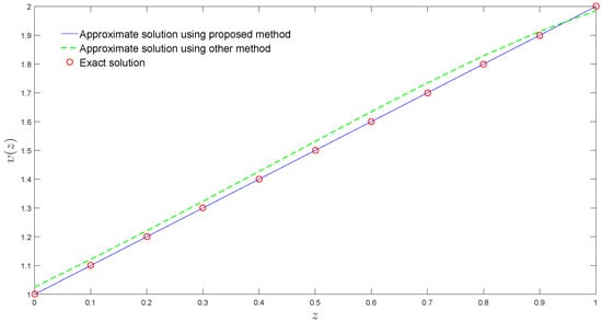
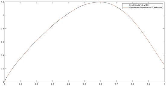
The numerical results computed using our method are compared with the method of [33] by choosing various n. We observe that our proposed method produces efficient numerical results as compared to the numerical results obtained by using the method of [33] (see Table 1 and Table 2 and Figure 1). Moreover, for a small value of , the exact solution and the approximate solution computed by using our method coincide (see Table 1 and Figure 1).
Table 1.
Comparison of approximate solution of Example 1.
Table 2.
Comparison of absolute errors of Example 1.
Figure 1.
Approximate solutions of Example 1 computed by our method at is compared with the method of [33] computed at .
Remark 2.
The numerical results of Example 1 computed at by using our method are compared with the results obtained by using the methods of [32,34] at . We observe that, for a small value of , the approximate solution obtained using our method coincides with the exact solution of Example 1 (see Table 3 and Table 4). However, the exact solution and the approximate solution computed by using the methods of [32,34] coincide at . This shows that our proposed method is numerically more efficient.
Table 3.
Comparison of approximate solution of Example 1.
Table 4.
Comparison of approximate solution of Example 1.
Example 2.
Consider the following linear initial value problem [38]:
The exact solution of the problem is [39].
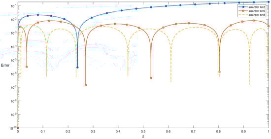
To solve the problem, we use the technique described in Section 4.1. The absolute error for and is shown in Table 5. An error plot is also shown in Figure 2 for these values.
Table 5.
Absolute error for and n = 2, 5 and 8 in Example 2.
Figure 2.
Error plots of Example 2 at different scale levels.
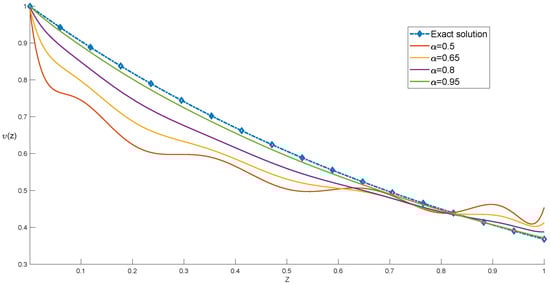
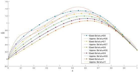
We can see in Table 5 that a good approximation has been achieved by using some initial terms of VLPs. Moreover, the numerical results for when and and 1 are plotted in Figure 3. The exact solution for is . It can be noted that the numerical solution converges to the analytical solution when α approaches 1. We also analyze the nonlocal behavior of the fractional derivative by computing the results at various non-integer values of α, which highlights the advantage of using the fractional derivatives, as the next state of the system depends not only upon its current state by also upon all of its historical states.
Figure 3.
Exact and approximate solutions of Example 2 are compared at different scale levels.
Example 3.
Consider the following initial value problem [10]:
subject to the initial condition with integer order
The source term is given as
The exact solution at is given below:
We test the behavior of our proposed method by solving Example (3) at various values of n. In Table 6, we list the and errors for different values of n. We compare the numerical results obtained by using our proposed method with the numerical results obtained in [10]. It can be observed that the errors computed by using our method are much smaller than those computed by using the method presented in [10]; see Table 6. This highlights the efficiency of our method for this problem. Note that the symbol means that the result for n is unavailable for the method [10].
Table 6.
Approximate results of Example 3 at various values of n.
Example 4.
Consider the following nonlinear initial value problem [40]:
The exact solution of the problem is [39].
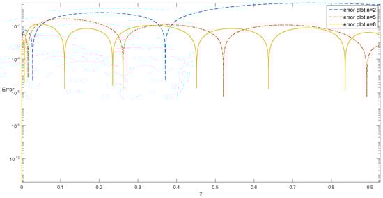
We have solved the problem using the technique described in Section 4.2. The absolute error for and is shown in Table 5. An error plot is also shown in Figure 4 and Figure 5 for these values. We can see in Table 7 that a good approximation has been achieved. Numerical results for when and and 1 are plotted in Figure 6, along with the exact solutions at the given values of α. It can be noted that, as α approaches 1, the solution of the FDEs approaches that of the integer-order differential equations. We also analyze the nonlocal behavior of the fractional derivative by computing the results at various non-integer values of α, which highlights the advantage of using the fractional derivatives, as the next state of the system depends not only upon its current state but also upon all of its historical states (Table 8).
Figure 4.
Error plots of Example 4 at different scale levels.
Figure 5.
Exact and approximate solutions of Example 4 are compared at n = 20.
Table 7.
Absolute error for and n = 2, 5 and 8 in Example 4.
Figure 6.
Exact and approximate solutions of Example 4 are compared at different scale levels.
Table 8.
Approximate results of Example 4 at various values of .
Example 5.
Consider the following nonlinear initial value problem:
We solved this problem by using the same technique as described in Section 4.2 with .
The exact solution of the problem is , whereas the source term is .
The operational matrices can be expressed as
where
Now, using the initial condition, we obtain three equations:
Meanwhile, using the technique in Section 4.2, we obtain the following equation:
Now, we collocate Equation (74) at the first root of and we obtain .
Example 6.
Consider the following non-homogenous multi-order fractional problem:
subject to the following initial conditions
The source term is as below:
The exact solution corresponding to , is given below:
We can observe in Example 6 that a good approximation of the function has been achieved while using as a scale level. The absolute error Table 9 at different scale levels is given below. (see Figure 7).
Table 9.
Absolute error for n = 2, 5 and 8 in Example 6.
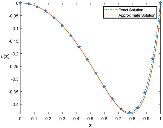
Figure 7.
Graphs of exact solution and approximate solution of Example 6 with .
Moreover, a comparison between the exact solution and approximate solution at different scale levels for the values of z is given in Table 10.
Table 10.
Comparison of exact solution with approximate solution (AS) at m = 2, 5 and 8 in Example 6.
7. Conclusions
In the present study, we introduce a new fractional-order derivative operational matrix of VLPs in Caputo sense. The newly derived operational matrix is used to develop a computer-oriented numerical algorithm to solve the linear and nonlinear FDEs that include the Caputo fractional-order derivative. The proposed numerical algorithm has the advantage of transforming the problems into a system of algebraic equations that are easy to solve using any computational software. To the best of our knowledge, this is the first result where the numerical algorithm is presented using the operational matrix of VLPs and the solution of the problems is approximated using its basis vectors.
We tested the accuracy and efficiency of the algorithm by solving various linear and nonlinear FDEs with initial conditions. We found that with an increase in the values of n, the approximate solutions were in good agreement with the exact solutions. We also demonstrated the high efficiency of the method by determining the amount of absolute error and observed that as we increased n, this amount was decreased significantly. In addition to this, the numerical efficiency was also demonstrated by comparing the results obtained by using our method with results obtained otherwise in the literature [10,32,33,34]. We observed that our method produced more efficient results.
Author Contributions
Conceptualization, I.T. and T.A.; Formal analysis, Z.A.N., I.T. and M.A.A.; Funding acquisition, T.A. and M.A.A.; Investigation, Z.A.N. and T.A.; Methodology, Z.A.N. and I.T.; Resources, T.A.; Software, Z.A.N. and I.T.; Supervision, I.T. and T.A.; Validation, I.T., T.A. and M.A.A.; Visualization, Z.A.N.; Writing—original draft, Z.A.N.; Writing—review and editing, I.T., T.A. and M.A.A. All authors contributed equally to this article. All authors read and approved the final manuscript.
Funding
This research received no external funding.
Institutional Review Board Statement
Not applicable.
Informed Consent Statement
Not applicable.
Acknowledgments
Prince Nourah bint Abdulrahman University Researchers supporting project number (PNURSP2022R14), Princess Nourah bint Abdulrahman University, Riyadh, Saudi Arabia. The author T. Abdeljawad would like to thank Prince Sultan University for paying the APC and for the support through the TAS research lab.
Conflicts of Interest
The authors declare no conflict of interest.
References
- Diethelm, K. The Analysis of Fractional Differential Equations: An Application-Oriented Exposition Using Differential Operators of Caputo Type; Springer Science & Business Media: New York, NY, USA, 2010. [Google Scholar]
- Eckert, M.; Kupper, M.; Hohmann, S. Functional fractional calculus for system identification of battery cells. AT-Automatisierungstechnik 2014, 62, 272–281. [Google Scholar] [CrossRef]
- Kilbas, A.A.; Srivastava, H.M.; Trujillo, J.J. Theory and Applications of Fractional Differential Equations; Elsevier: Amsterdam, The Netherlands, 2006; Volume 204. [Google Scholar]
- Miller, K.S.; Ross, B. An Introduction to the Fractional Calculus and Fractional Differential Equations; Wiley: Hoboken, NJ, USA, 1993. [Google Scholar]
- Alam, M.; Talib, I.; Bazighifan, O.; Chalishajar, D.; Almarri, B. An analytical technique implemented in the fractional Clannish Random Walker’s Parabolic equation with nonlinear physical phenomena. Mathematics 2021, 9, 801. [Google Scholar] [CrossRef]
- Oldham, K.B.; Spanier, J. The Fractional Calculus; Academic Press: New York, NY, USA, 1974. [Google Scholar]
- Zhang, H.; Jiang, X.; Yang, X. A time-space spectral method for the time-space fractional Fokker-Planck equation and its inverse problem. Appl. Math. Comput. 2018, 320, 302–318. [Google Scholar] [CrossRef]
- Zhang, H.; Jiang, X.; Zeng, F.; Karniadakis, G.E. A stabilized semi-implicit Fourier spectral method for nonlinear space-fractional reaction-diffusion equations. J. Comput. Phys. 2020, 405, 109141. [Google Scholar] [CrossRef] [Green Version]
- Zheng, X.; Wang, H. Optimal-order error estimates of finite element approximations to variable-order time-fractional diffusion equations without regularity assumptions of the true solutions. IMA J. Numer. Anal. 2021, 41, 1522–1545. [Google Scholar] [CrossRef]
- Talaei, Y.; Asgari, M. An operational matrix based on Chelyshkov polynomials for solving multi-order fractional differential equations. Neural Comput. Appl. 2018, 30, 1369–1376. [Google Scholar] [CrossRef]
- Fazli, H.; Nieto, J.J. An investigation of fractional Bagley-Torvik equation. Open Math. 2019, 17, 499–512. [Google Scholar] [CrossRef]
- Pang, D.; Jiang, W.; Du, J.; Niazi, A. Analytical solution of the generalized Bagley-Torvik equation. Adv. Differ. Equ. 2019, 2019, 1–13. [Google Scholar] [CrossRef]
- Abbas, M.I. Existence and uniqueness results for fractional order differential equations with Riemann-Liouville fractional integral boundary conditions. Abstr. Appl. Anal. 2015, 2015, 1–7. [Google Scholar]
- Deng, J.; Ma, L. Existence and uniqueness of solutions of initial value problems for nonlinear fractional differential equations. Appl. Math. Lett. 2010, 23, 676–680. [Google Scholar] [CrossRef] [Green Version]
- Khan, R.A.; Rehman, M.; Henderson, J. Existence and uniqueness of solution for nonlinear fractional differential equations with integral boundary conditions. Fract. Differ. Calc. 2011, 1, 29–43. [Google Scholar] [CrossRef] [Green Version]
- Liu, X.; Jia, M.; Wu, B. Existence and uniqueness of solution for fractional differential equations with integral boundary conditions. Electron. J. Qual. Differ. Equ. 2009, 2009, 69. [Google Scholar] [CrossRef]
- Zhou, Y. Existence and uniqueness of solutions for a system of fractional differential equations. Fract. Calc. Appl. Anal. 2009, 12, 195–204. [Google Scholar]
- Kazem, S.; Abbasbandy, S.; Kumar, S. Fractional-order Legendre functions for solving fractional-order differential equations. Appl. Math. Model. 2013, 37, 5498–5510. [Google Scholar] [CrossRef]
- Saadatmandi, A.; Dehghan, M. A new operational matrix for solving fractional-order differential equations. Comput. Math. Appl. 2010, 59, 1326–1336. [Google Scholar] [CrossRef] [Green Version]
- Song, L.; Wang, W. A new improved Adomian decomposition method and its application to fractional differential equations. Appl. Math. Model. 2013, 37, 1590–1598. [Google Scholar] [CrossRef]
- Talib, I.; Alam, M.; Baleanu, D.; Zaidi, D.; Marriyam, A. A new integral operational matrix with applications to multi-order fractional differential equations. AIMS Math. 2021, 6, 8742–8771. [Google Scholar] [CrossRef]
- Benattia, M.E.; Belghaba, K. Numerical Solution for Solving Fractional Differential Equations using Shifted Chebyshev Wavelet. Gen. Lett. Math. 2017, 3, 101–110. [Google Scholar]
- Darani, M.A.; Saadatmandi, A. The operational matrix of fractional derivative of the fractional-order Chebyshev functions and its applications. Comput. Methods Differ. Equ. 2017, 5, 67–87. [Google Scholar]
- Khalil, H.; Khan, R.A.; Al-Smadi, M.H.; Freihat, A.A.; Shawagfeh, N. New Operational Matrix for Shifted Legendre Polynomials and Fractional Differential Equations with Variable Coeffcients; Punjab University Journal of Mathematics: Lahore, Pakistan, 2020; Volume 47. [Google Scholar]
- Bhrawy, A.H.; Alofi, A.S. The operational matrix of fractional integration for shifted Chebyshev polynomials. Appl. Math. Lett. 2013, 26, 25–31. [Google Scholar] [CrossRef] [Green Version]
- Talib, I.; Tunc, C.; Noor, Z.A. New operational matrices of orthogonal Legendre polynomials and their operational. J. Taibah Univ. Sci. 2019, 13, 377–389. [Google Scholar] [CrossRef] [Green Version]
- Rahimkhani, P.; Ordokhani, Y.; Babolian, E. A new operational matrix based on Bernoulli wavelets for solving fractional delay differential equations. Numer. Algorithms 2017, 74, 223–245. [Google Scholar] [CrossRef]
- Dehestani, H.; Ordokhani, Y.; Razzaghi, M. Combination of Lucas wavelets with Legendre-Gauss quadrature for fractional Fredholm-Volterra integro-differential equations. J. Comput. Appl. Math. 2021, 382, 113070. [Google Scholar] [CrossRef]
- Dehestani, H.; Ordokhani, Y.; Razzaghi, M. Fractional-order Bessel functions with various applications. Appl. Math. 2019, 64, 637–662. [Google Scholar] [CrossRef]
- Dehestani, H.; Ordokhani, Y.; Razzaghi, M. Numerical technique for solving fractional generalized pantograph-delay differential equations by using fractional-order hybrid bessel functions. Int. J. Appl. Comput. Math. 2020, 6, 1–27. [Google Scholar] [CrossRef]
- Dehestani, H.; Ordokhani, Y.; Razzaghi, M. On the applicability of Genocchi wavelet method for different kinds of fractional-order differential equations with delay. Numer. Linear Algebra Appl. 2019, 26, 2259. [Google Scholar] [CrossRef]
- Gulsu, M.; Ozturk, Y.; Ayse, A. Numerical solution of the fractional Bagley-Torvik equation arising in fluid mechanics. Int. J. Comput. Math. 2017, 94, 173–184. [Google Scholar] [CrossRef]
- Raja, M.; Khan, J.A.; Qureshi, I. Solution of fractional order system of Bagley-Torvik equation using evolutionary computational intelligence. Math. Probl. Eng. 2011, 2011, 675075. [Google Scholar] [CrossRef] [Green Version]
- Yuzbasi, S. Numerical solution of the Bagley-Torvik equation by the Bessel collocation method. Math. Methods Appl. Sci. 2013, 36, 300–312. [Google Scholar] [CrossRef]
- Agarwal, P.; El-Sayed, A.A. Vieta-Lucas polynomials for solving a fractional-order mathematical physics model. Adv. Differ. Equ. 2020, 2020, 1–18. [Google Scholar] [CrossRef]
- Canuto, C.; Hussaini, M.Y.; Quarteroni, A.; Zang, T.A. Spectral Methods: Fundamentals in Single Domains; Springer Science & Business Media: New York, NY, USA, 2007. [Google Scholar]
- Stewart, J. Single Variable Essential Calculus: Early Transcendentals; Cengage Learning: Belmont, CA, USA, 2012. [Google Scholar]
- Hashim, I.; Abdulaziz, O.; Momani, S. Homotopy analysis method for fractional IVPs. Commun. Nonlinear Sci. Numer. Simul. 2009, 14, 674–684. [Google Scholar] [CrossRef]
- Diethelm, K.; Ford, N.J.; Freed, A.D. A predictor-corrector approach for the numerical solution of fractional differential equations. Nonlinear Dyn. 2002, 29, 3–22. [Google Scholar] [CrossRef]
- Kumar, P.; Agrawal, O.P. An approximate method for numerical solution of fractional differential equations. Signal Process. 2006, 86, 2602–2610. [Google Scholar] [CrossRef]
Publisher’s Note: MDPI stays neutral with regard to jurisdictional claims in published maps and institutional affiliations. |
© 2022 by the authors. Licensee MDPI, Basel, Switzerland. This article is an open access article distributed under the terms and conditions of the Creative Commons Attribution (CC BY) license (https://creativecommons.org/licenses/by/4.0/).