Author Contributions
Conceptualization, M.Y., Q.U.N.A. and S.K.; methodology, Q.U.N.A. and R.G.; validation, R.G. and S.K.; formal analysis, M.Y., Q.U.N.A. and S.K.; investigation, S.K; writing—original draft preparation, Q.U.N.A.; writing—review and editing, M.Y., R.G. and S.K.; supervision, R.G. and M.Y.; project administration, R.G.; funding acquisition, R.G. All authors have read and agreed to the published version of the manuscript.
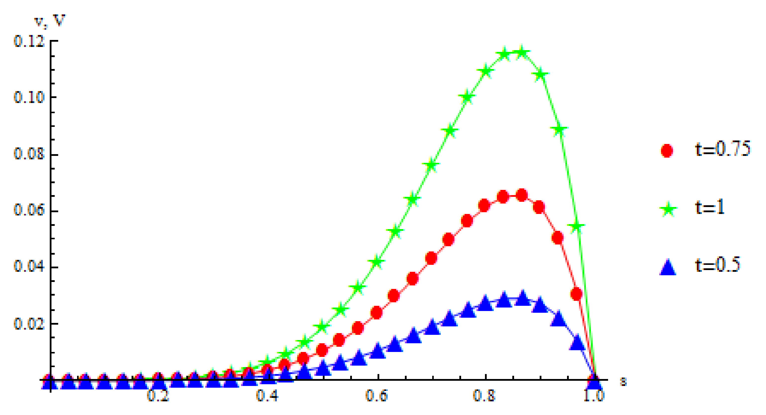
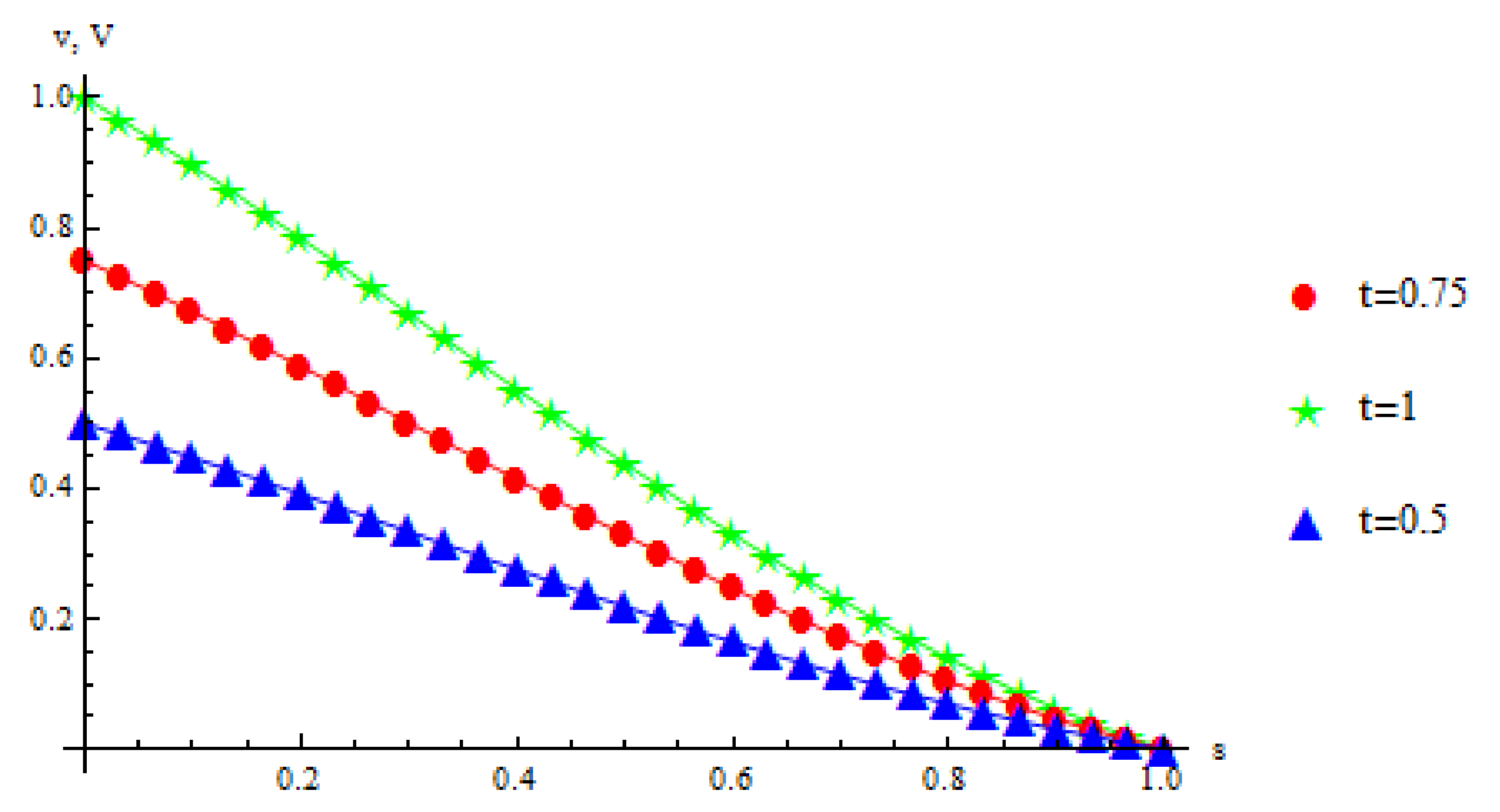
Figure 1.
The exact and approximate (triangles, stars, circles) solutions using cubic B-spline-based scheme for Example 1 at various times when .
Figure 1.
The exact and approximate (triangles, stars, circles) solutions using cubic B-spline-based scheme for Example 1 at various times when .
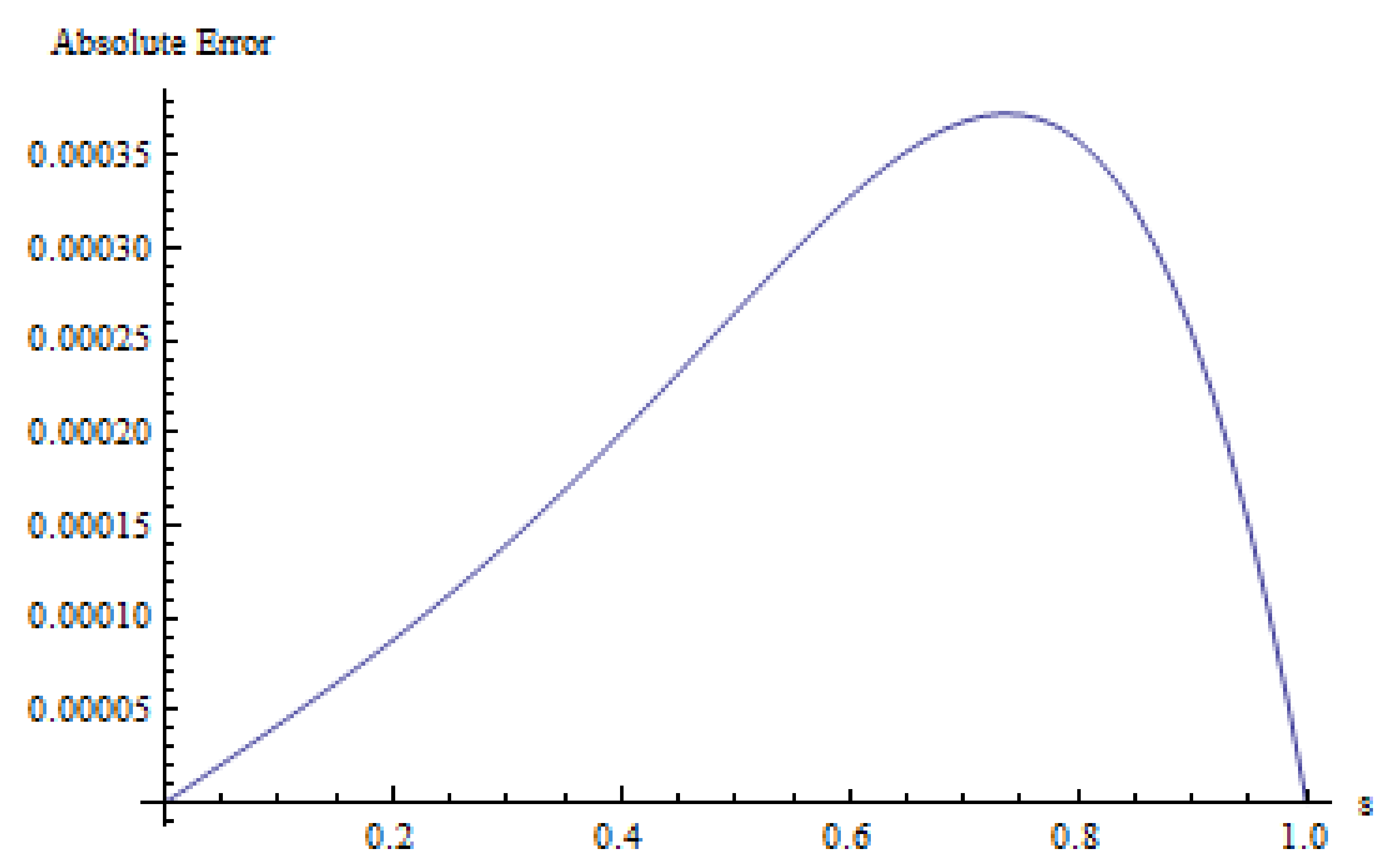
Figure 2.
The 2D error profile using cubic B-spline-based scheme for Example 1 when , , , .
Figure 2.
The 2D error profile using cubic B-spline-based scheme for Example 1 when , , , .
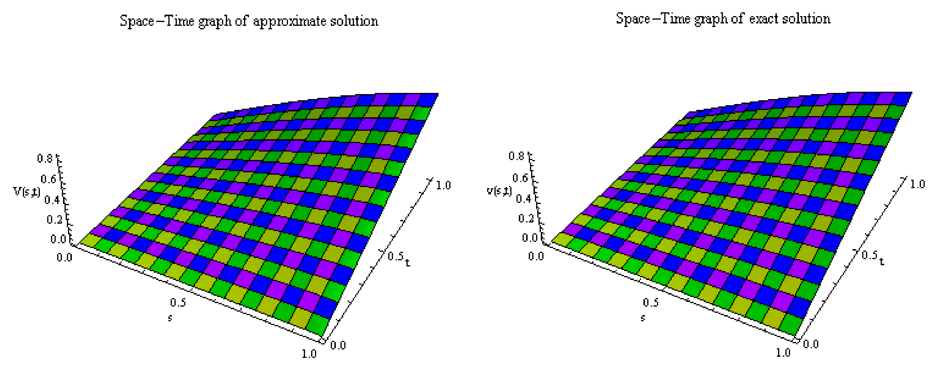
Figure 3.
The approximate (left) and exact (right) solutions using cubic B-spline-based scheme for Example 1 when , , , .
Figure 3.
The approximate (left) and exact (right) solutions using cubic B-spline-based scheme for Example 1 when , , , .
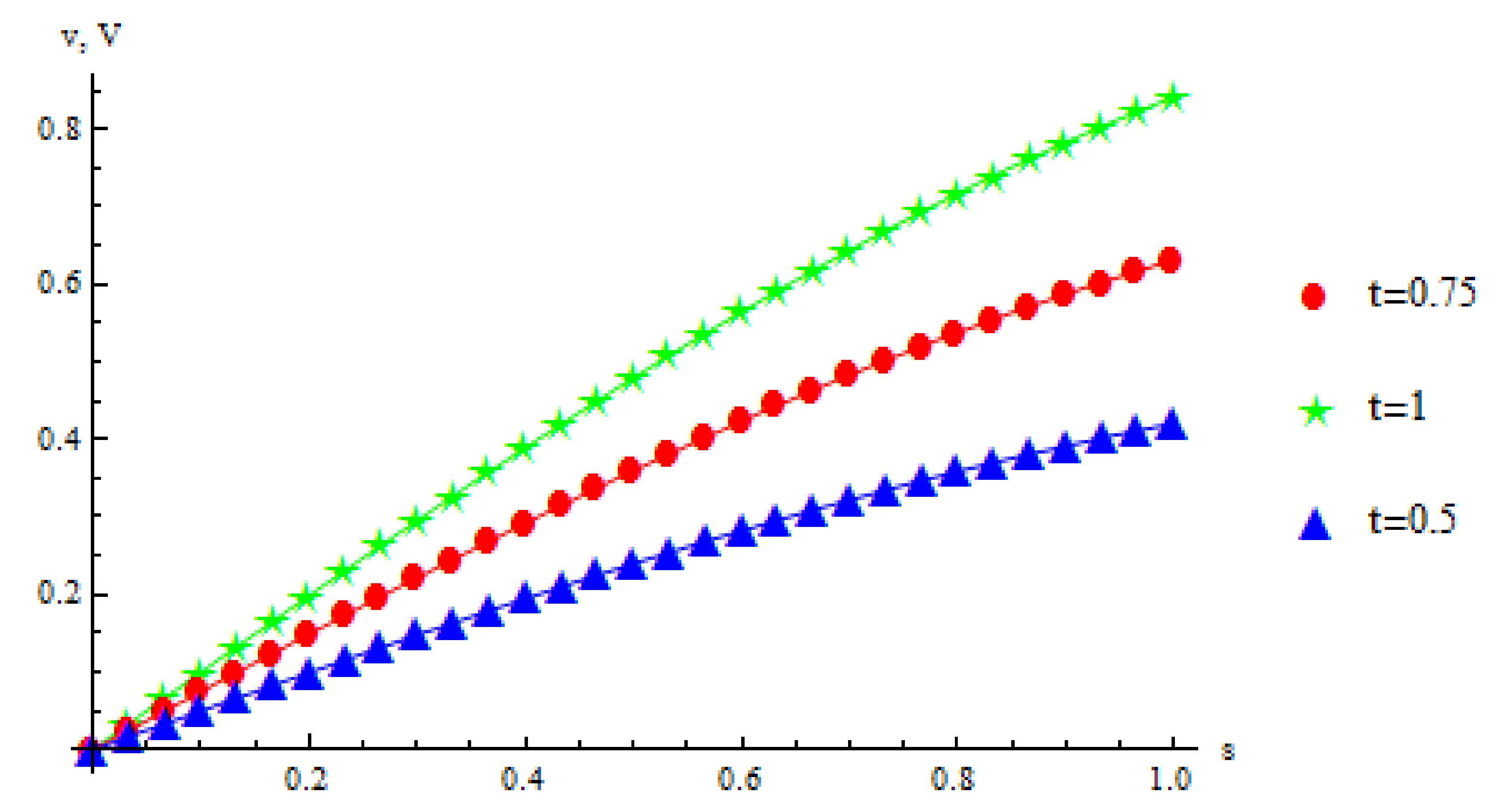
Figure 4.
The exact and approximate (triangles, stars, circles) solutions using cubic B-spline-based scheme for Example 2 at various times when .
Figure 4.
The exact and approximate (triangles, stars, circles) solutions using cubic B-spline-based scheme for Example 2 at various times when .
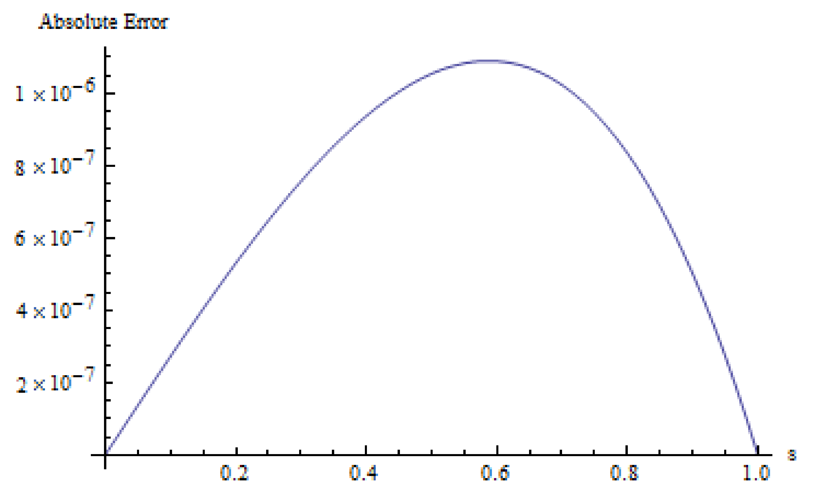
Figure 5.
The 2D error profile using cubic B-spline-based scheme for Example 2 when , , , .
Figure 5.
The 2D error profile using cubic B-spline-based scheme for Example 2 when , , , .
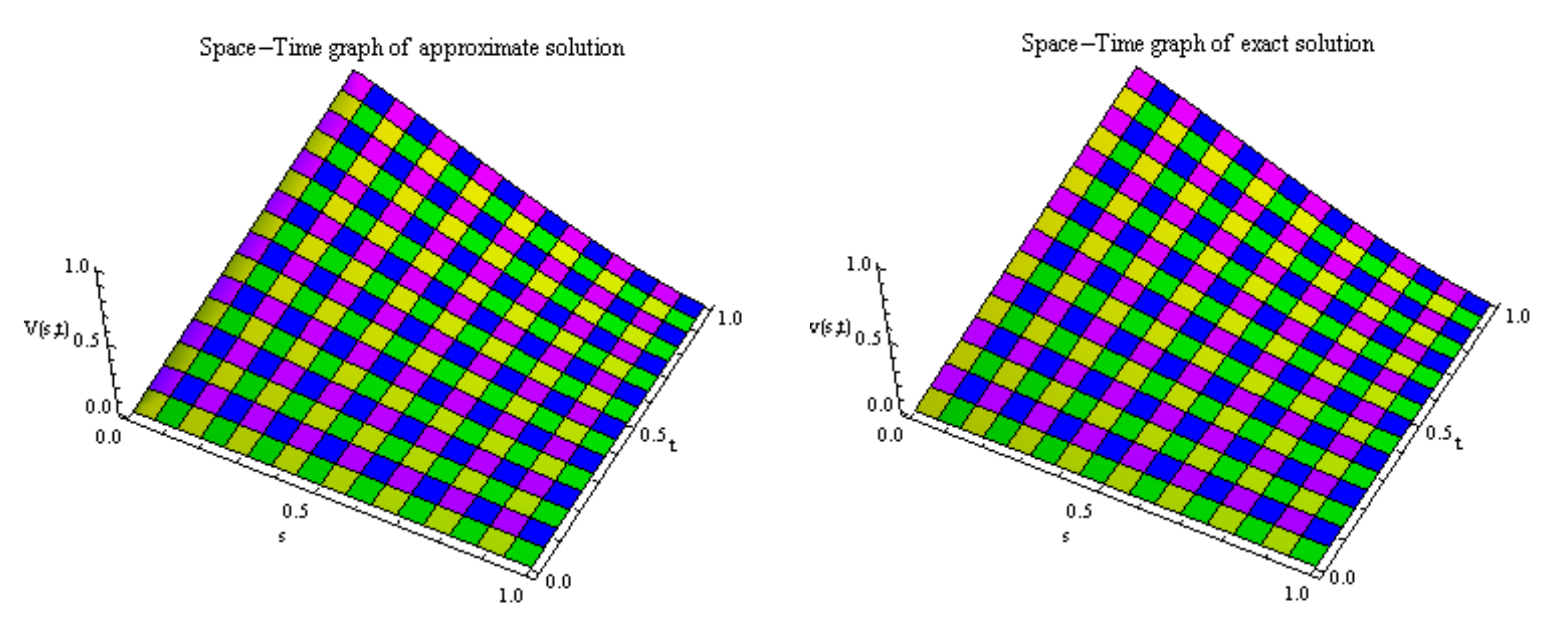
Figure 6.
The approximate (left) and exact (right) solutions using cubic B-spline-based scheme for Example 2 when , , , .
Figure 6.
The approximate (left) and exact (right) solutions using cubic B-spline-based scheme for Example 2 when , , , .
Figure 7.
The exact and approximate (triangles, stars, circles) solutions using cubic B-spline-based scheme for Example 3 at various times when .
Figure 7.
The exact and approximate (triangles, stars, circles) solutions using cubic B-spline-based scheme for Example 3 at various times when .
Figure 8.
The 2D error profile using cubic B-spline-based scheme when for Example 2 when , , , .
Figure 8.
The 2D error profile using cubic B-spline-based scheme when for Example 2 when , , , .
Figure 9.
The approximate (left) and exact (right) solutions using cubic B-spline-based scheme for Example 3 when , , , .
Figure 9.
The approximate (left) and exact (right) solutions using cubic B-spline-based scheme for Example 3 when , , , .
Table 1.
Comparison of errors using various B-splines when for Example 1.
Table 1.
Comparison of errors using various B-splines when for Example 1.
| M | CuBS | TCuBS | ECuBS |
|---|
| | Norm | Norm | Norm | Norm | Norm | Norm |
|---|
| 20 | | | | | | |
| 40 | | | | | | |
| 80 | | | | | | |
| 160 | | | | | | |
Table 2.
Comparison of errors using various B-splines with for Example 1.
Table 2.
Comparison of errors using various B-splines with for Example 1.
| M | CuBS | TCuBS | ECuBS |
|---|
| | Norm | Norm | Norm | Norm | Norm | Norm |
|---|
| 20 | | | | | | |
| 40 | | | | | | |
| 80 | | | | | | |
| 160 | | | | | | |
Table 3.
Comparison of errors using various B-splines with for Example 1.
Table 3.
Comparison of errors using various B-splines with for Example 1.
| M | CuBS | TCuBS | ECuBS |
|---|
| | Norm | Norm | Norm | Norm | Norm | Norm |
|---|
| 20 | | | | | | |
| 40 | | | | | | |
| 80 | | | | | | |
| 160 | | | | | | |
Table 4.
Comparison of errors using various B-splines with for Example 2.
Table 4.
Comparison of errors using various B-splines with for Example 2.
| M | CuBS | TCuBS | ECuBS |
|---|
| | Norm | Norm | Norm | Norm | Norm | Norm |
|---|
| 20 | | | | | | |
| 40 | | | | | | |
| 80 | | | | | | |
| 160 | | | | | | |
Table 5.
Comparison of errors using various B-splines with for Example 2.
Table 5.
Comparison of errors using various B-splines with for Example 2.
| M | CuBS | TCuBS | ECuBS |
|---|
| | Norm | Norm | Norm | Norm | Norm | Norm |
|---|
| 20 | | | | | | |
| 40 | | | | | | |
| 80 | | | | | | |
| 160 | | | | | | |
Table 6.
Comparison of errors using various B-splines with for Example 2.
Table 6.
Comparison of errors using various B-splines with for Example 2.
| M | CuBS | TCuBS | ECuBS |
|---|
| | Norm | Norm | Norm | Norm | Norm | Norm |
|---|
| 20 | | | | | | |
| 40 | | | | | | |
| 80 | | | | | | |
| 160 | | | | | | |
Table 7.
Comparison of errors using various B-splines with for Example 3.
Table 7.
Comparison of errors using various B-splines with for Example 3.
| M | CuBS | TCuBS | ECuBS |
|---|
| | Norm | Norm | Norm | Norm | Norm | Norm |
|---|
| 20 | | | | | | |
| 40 | | | | | | |
| 80 | | | | | | |
| 160 | | | | | | |
Table 8.
Comparison of errors using various B-splines with for Example 3.
Table 8.
Comparison of errors using various B-splines with for Example 3.
| M | CuBS | TCuBS | ECuBS |
|---|
| | Norm | Norm | Norm | Norm | Norm | Norm |
|---|
| 20 | | | | | | |
| 40 | | | | | | |
| 80 | | | | | | |
| 160 | | | | | | |
Table 9.
Comparison of errors using various B-splines with for Example 3.
Table 9.
Comparison of errors using various B-splines with for Example 3.
| M | CuBS | TCuBS | ECuBS |
|---|
| | Norm | Norm | Norm | Norm | Norm | Norm |
|---|
| 20 | | | | | | |
| 40 | | | | | | |
| 80 | | | | | | |
| 160 | | | | | | |


