On Variable-Order Fractional Discrete Neural Networks: Solvability and Stability

Abstract

Few papers have been published to date regarding the stability of neural networks described by fractional difference operators. This paper makes a contribution to the topic by presenting a variable-order fractional discrete neural network model and by proving its Ulam–Hyers stability. In particular, two novel theorems are illustrated, one regarding the existence of the solution for the proposed variable-order network and the other regarding its Ulam–Hyers stability. Finally, numerical simulations of three-dimensional and two-dimensional variable-order fractional neural networks were carried out to highlight the effectiveness of the conceived theoretical approach.

1. Introduction

Fractional calculus deals with non-integer-order differential equations or non-integer-order difference equations [1]. It is worth noting that, while the first known reference of fractional derivatives can be found in the correspondence of G. W. Leibniz and Marquis de l’Hospital in 1695, fractional difference operators were introduced only in 1974 [2]. Consequently, non-integer-order discrete-time systems have received less attention in the literature with respect to non-integer-order continuous-time systems [1].

Referring to fractional continuous/discrete systems, some manuscripts in the literature have investigated their stability properties [3,4,5,6,7,8,9]. For example, in [3], an extension of the Mikhailov stability criterion to fractional discrete systems described by the nabla Grünwald–Letnikov operator was introduced. The stability methods in [3] are efficient from the computational point of view and can be applied to both commensurate and incommensurate systems. In [4], a novel definition of the Mittag–Leffler stability for discrete fractional systems was introduced. In particular, some useful criteria were developed in order to ensure the stability of nabla discrete fractional systems for both the Caputo definition and the Riemann–Liouville definition. In [5], the stability and synchronization for some fractional-order difference equations were investigated. In [9], the fractional delay discrete systems were studied using a discrete delayed Mittag–Leffler matrix function. Moreover, a criterion on the finite-time stability of fractional delay difference equations with constant coefficients was derived.

It is worth noting that very few papers have been published in the literature regarding the Ulam–Hyers stability in fractional discrete systems [10,11,12]. For example, in [10], the Ulam–Hyers stability of linear and non-linear nabla fractional Caputo difference equations on finite intervals was investigated. In [11], the Ulam–Hyers stability for Riemann–Liouville fractional nabla difference equations was studied. In [12], the Hyers–Ulam stability of an inverted pendulum modeled by a discrete fractional Duffing equation was investigated.

Among the different types of non-integer-order discrete-time dynamical systems, an important class is represented by neural networks described by non-integer-order difference operators [13,14,15,16,17,18,19,20,21]. Even though the stability of fractional discrete neural networks is a prerequisite for their successful applications [13], few papers have been published to date on the topic. For example, in [14], the global Mittag–Leffler stability and the finite-time stability of fractional discrete neural networks (in the complex field) were studied for two different types of activation functions. In [15], a fractional discrete quaternion-valued memristive neural network was introduced. Then, a sufficient condition to ensure the quasi-stability of the network equilibrium point was illustrated. In [16], Lyapunov’s direct method was utilized to ensure the stability of fractional discrete complex-valued neural networks, whereas in [17], the stability and synchronization of non-integer-order discrete neural networks with time delays were studied. In [18], the fixed-point theorem was exploited to derive some stability conditions for fractional difference equations. Then, the obtained stability results were applied to fractional discrete neural networks with and without delay. In [19], the exponential stability of non-integer-order discrete quaternion-valued neural networks was investigated. In particular, the Lyapunov–Krasovskii functional and matrix inequality were utilized to prove the exponential stability of the network equilibrium point. In [20], the Arzela–Ascoli theorem was exploited to ensure the finite-time stability of fractional discrete complex-valued neural networks. Finally, referring to variable-order fractional discrete neural networks (i.e., networks where the fractional order changes over discrete time), an attempt to study their stability was carried out in [21]. However, the results in [21] were related to the Mittag–Leffler stability. No result is available in the literature regarding the Ulam–Hyers stability of fractional discrete neural networks, including those with a variable order.

Based on the absence in the literature mentioned above, this paper makes a contribution to the topic of the stability of fractional discrete neural networks by presenting a variable-order model based on the Caputo h-difference operator and by proving its Ulam–Hyers stability. In particular, two novel theorems are illustrated, one regarding the existence of the solution for the proposed variable-order network and the other regarding its Ulam–Hyers stability. The paper is organized as follows. In Section 2, the background on fractional discrete calculus is provided. In Section 3, the equations of the proposed variable-order fractional discrete neural network are introduced. In Section 4, a novel theorem is presented, with the aim to prove the existence of the solution for the considered neural network model. In Section 5, the Ulam–Hyers stability of the proposed variable-order fractional discrete neural network is proven by means of a novel theorem. Finally, in Section 6, numerical simulations of three-dimensional and two-dimensional variable-order fractional neural networks are carried out to highlight the effectiveness of the conceived theoretical approach.

2. Background on Fractional Discrete Calculus

The following definitions for discrete fractional calculus are introduced.

Definition 1

(Fractional sum [22]). Let $x:{\left(h\mathbb{N}\right)}_a\to \mathbb{R}\mathrm{and}0<v$ be given. a is a starting point. The $v-$th order h-sum is given by:

$${}_h{\Delta }_a^{-v}x\left(t\right)={\displaystyle \frac{h}{\Gamma \left(v_{}\right)}}\sum _{s=\frac{a}{h}}^{\frac{t}{h}-v_{}}{(t-\sigma \left(sh\right))}_h^{v_{}-1}x\left(sh\right),\sigma \left(sh\right)=(s+1)h,t\in {\left(h\mathbb{N}\right)}_{a+vh}$$

where the h-falling factorial function is defined as:

$$t_h^{\left(v\right)}=h^v{\displaystyle \frac{\Gamma (\frac{t}{h}+1)}{\Gamma (\frac{t}{h}+1-v)}},t,v\in \mathbb{R}$$

while ${\left(h\mathbb{N}\right)}_{a+(1-v)h}=\{a+(1-v)h,a+(2-v)h,\dots \}$.

Definition 2

(Caputo delta difference [22]). For $x\left(t\right)$ defined on ${\left(h\mathbb{N}\right)}_a$ and $0<\alpha$, the Caputo-like difference is defined by:

$${}_h^C{\Delta }_a^{\alpha }x\left(t\right)={\Delta }_a^{-(m-\alpha )}{\Delta }_h^{m}x\left(t\right),t\in {\left(h\mathbb{N}\right)}_{a+(m-\alpha )h}$$

where ${\Delta }_{h}x\left(t\right)={\displaystyle \frac{x(t+h)-x\left(t\right)}{h}}$ and $m=\left[\alpha \right]+1$.

If the fractional order α is a positive integer m, then we have the following definition:

$${}_h^C{\Delta }_a^{\alpha }x\left(t\right)={\Delta }_h^{m}x\left(t\right),t\in {\left(h\mathbb{N}\right)}_a.$$

Lemma 1

([22]). In what follows, some useful proprieties used in this paper are reported:

• Discrete Leibniz integral law:

  $${}_h{\Delta }_{a+(1-v)h}^{-v}{}_h^C{\Delta }_a^{v}x\left(t\right)=x\left(t\right)-x\left(a\right),0<v\le 1,t\in {\left(h\mathbb{N}\right)}_{a+h};$$
• Fractional Caputo difference of a constant c:

  $${}_h^C{\Delta }_a^{v}c=0,0<v\le 1;$$
• Delta difference of the h–falling factorial function:

  $${\Delta }_s{(t-sh)}_h^{\left(v\right)}=-v{(t-\sigma \left(sh\right))}_h^{(v-1)}.$$

Lemma 2

(Arzela–Ascoli’s theorem [23]). A bounded, uniformly Cauchy subset Ω of Banach space E is relatively compact.

Lemma 3

(Krasnoselskii fixed-point theorem [23]). Let Ω be a nonempty, closed, convex, and bounded subset of Banach space E. Suppose that S, T are two operators, such that:

(i)

S is a contraction;

(ii)

For any $x,y\in \mathsf{\Omega },Sx+Ty\in \mathsf{\Omega }$;

(iii)

T is continuous, and $B\left(\mathsf{\Omega }\right)$ is relatively compact.

Then, for $x\in \mathsf{\Omega }$, the operator equation $Sx+Tx=x$ has a solution.

3. Variable-Order Fractional Discrete Neural Network

Discrete-time fractional-order neural networks are well suited to modeling the dynamics of fractional-order discrete non-linear systems. In reality, because they have modeling capabilities to a required precision, they are considered a contender for a generic, parametric, non-linear model of a large class of discrete non-linear systems with a fractional order. In this paper, we explore a type of variable-order fractional discrete neural network described by:

$${}_h^C{\Delta }_{t_{kl}}^{v_k}x\left(t\right)=-Ax(t+v_{k}h)+Bf(t;x(t+v_{k}h)),$$

(1)

where (1) can be reduced as:

$$\left\{\begin{array}{c}{}_h^C{\Delta }_{t_0}^{v_0}x\left(t\right)=-Ax(t+v_{0}h)+Bf(t;x(t+v_{0}h)),t\in \{t_0+(1-v_0)h,\dots ,t_l-v_{0}h\}\hfill \\ {}_h^C{\Delta }_{t_l}^{v_1}x\left(t\right)=-Ax(t+v_{1}h)+Bf(t;x(t+v_{1}h)),t\in \{t_l+(1-v_1)h,\dots ,t_{2l}-v_{1}h\}\hfill \\ \dots \hfill \\ {}_h^C{\Delta }_{t_{kl}}^{v_k}x\left(t\right)=-Ax(t+v_{k}h)+Bf(t;x(t+v_{k}h)),t\in \{t_{kl}+(1-v_k)h,\dots ,t_{(k+1)l}-v_{k}h\}\hfill \end{array}\right.$$

(2)

in which $t\in {\left(h\mathbb{N}\right)}_{t_{kl}+(1-v_k)h},0<v_k\le 1,k=0,\dots ,m-1,m$ is the number of intervals, ${}_h^C{\Delta }_{t_{kl}}^{v_k}$ denotes the variable-order fractional Caputo h-difference operator of order $v_k$, $x\left(t\right)={(x_1\left(t\right),\dots ,x_p\left(t\right))}^T\in {\mathbb{R}}^p$ is the state of the unit at time t, p is the dimension, $A=diag(-a_1,\dots ,-a_p)$, where $a_i>0$ represents the matrix with which the neurons will reset their potentials to the resting state when disconnected from the network, while $B\in {\mathbb{R}}_{p\times p}$ corresponds to the connection weights, and finally, $f(t,x\left(t\right))\in C({\left(h\mathbb{N}\right)}_{t_{kl}+(1-v_k)h},{\mathbb{R}}^p)$ is the activation function.

Lemma 4.

A function $x\left(t\right)$ is called the solution of (1) if $x\left(t\right)$ satisfies:

$$x\left(t\right)=\left\{\begin{array}{c}x\left(t_0\right)+{\displaystyle \frac{h}{\Gamma \left(v_0\right)}}\sum _{s=\frac{t_0}{h}+1-v_0}^{\frac{t}{h}-v_0}{(t-\sigma \left(sh\right))}_h^{v_0-1}[-Ax\left(sh\right)+Bf(sh,x\left(sh\right))],t\in \{t_0+h,\dots ,t_l\}\hfill \\ x\left(t_0\right)+\sum _{n=1}^{m-1}{\displaystyle \frac{h}{\Gamma \left(v_{n-1}\right)}}\sum _{s=\frac{t_{(n-1)l}}{h}+1-v_{n-1}}^{\frac{t_{nl}}{h}-v_{n-1}}{(t_{nl}-\sigma \left(sh\right))}_h^{v_{n-1}-1}[-Ax\left(sh\right)+Bf(sh,x\left(sh\right))]\hfill \\ +{\displaystyle \frac{h}{\Gamma \left(v_{m-1}\right)}}\sum _{s=\frac{t_{(m-1)l}}{h}+1-v_{m-1}}^{\frac{t}{h}-v_{m-1}}{(t-\sigma \left(sh\right))}_h^{v_{m-1}-1}[-Ax\left(sh\right)+Bf(sh,x\left(sh\right))],t\in \{t_{(m-1)l}+h,\dots ,t_{ml}\}.\hfill \end{array}\right.$$

(3)

Proof. 

Actually, the system (2) is equivalent to:

$$\left\{\begin{array}{c}x\left(t\right)=x\left(t_0\right)+{}_h{\Delta }_{t_0+(1-v_0)h}^{-v_0}[-Ax\left(t\right)+Bf(t,x\left(t\right))],t\in \{t_0+h,\dots ,t_l\}\hfill \\ x\left(t\right)=x\left(t_l\right)+{}_h{\Delta }_{t_l+(1-v_1)h}^{-v_1}[-Ax\left(t\right)+Bf(t,x\left(t\right))],t\in \{t_l+h,\dots ,t_{2l}\}\hfill \\ \dots \hfill \\ x\left(t\right)=x\left(t_{(m-1)l}\right)+{}_h{\Delta }_{t_{(m-1)l}+(1-v_{m-1})h}^{-v_{(m-1)}}[-Ax\left(t\right)+Bf(t,x\left(t\right))],t\in \{t_{(m-1)l}+h,\dots ,t_{ml}\}.\hfill \end{array}\right.$$

As for $k=0,t\in \{t_0+(1-v_0)h,\dots ,t_l-v_{0}h\}$, we obtain that the solution of (1) can be expressed as:

$$x\left(t\right)=x\left(t_0\right)+{}_h{\Delta }_{t_0+(1-v_0)h}^{-v_0}[-Ax\left(t\right)+Bf(t,x\left(t\right))].$$

We can further obtain:

$$x\left(t\right)=x\left(t_0\right)+{\displaystyle \frac{h}{\Gamma \left(v_0\right)}}\sum _{s=\frac{t_0}{h}+1-v_0}^{\frac{t}{h}-v_0}{(t-\sigma \left(sh\right))}_h^{v_0-1}[-Ax\left(sh\right)+Bf(sh,x\left(sh\right))],$$

and we can have $x\left(t_l\right)=x\left(t_0\right)+{\displaystyle \frac{h}{\Gamma \left(v_0\right)}}{\sum }_{s=\frac{t_0}{h}+1-v_0}^{\frac{t_l}{h}-v_0}{(t_l-\sigma \left(sh\right))}_h^{v_0-1}[-Ax\left(sh\right)+Bf(sh,x\left(sh\right))]$ as an initial condition of:

$${}_h^C{\Delta }_{t_l}^{v_1}x\left(t\right)=-Ax(t+v_{1}h)+Bf(t;x(t+v_{1}h)),t\in \{t_l+(1-v_1)h,\dots ,t_{2l}-v_{1}h\}.$$

Using the same approach, we can obtain the expression of $x\left(t\right)$ for any $t\in \{t_l+(1-v_1)h,\dots ,t_{2l}-v_{1}h\}$. In other words, we can have:

$$\begin{array}{cc}\hfill x\left(t\right)& =x\left(t_l\right)+{\displaystyle \frac{h}{\Gamma \left(v_1\right)}}\sum _{s=\frac{t_0}{h}+1-v_1}^{\frac{t}{h}-v_1}{(t-\sigma \left(sh\right))}_h^{v_1-1}[-Ax\left(sh\right)+Bf(sh,x\left(sh\right))]\hfill \\ \hfill & =x\left(t_0\right)+{\displaystyle \frac{h}{\Gamma \left(v_0\right)}}\sum _{s=\frac{t_0}{h}+1-v_0}^{\frac{t_l}{h}-v_0}{(t_l-\sigma \left(sh\right))}_h^{v_0-1}[-Ax\left(sh\right)+Bf(sh,x\left(sh\right))]\hfill \\ \hfill & +{\displaystyle \frac{h}{\Gamma \left(v_1\right)}}\sum _{s=\frac{t_l}{h}+1-v_1}^{\frac{t}{h}-v_1}{(t-\sigma \left(sh\right))}_h^{v_1-1}[-Ax\left(sh\right)+Bf(sh,x\left(sh\right))].\hfill \end{array}$$

Now, for any $t\in \{t_{kl}+(1-v_k)h,\dots ,t_{(k+1)l-v_{k}h}\},k=2,3,\dots ,m-1$, we can similarly derive $x\left(t\right)$ as follows:

$$x\left(t\right)=\left\{\begin{array}{c}x\left(t_0\right)+{\displaystyle \frac{h}{\Gamma \left(v_0\right)}}\sum _{s=\frac{t_0}{h}+1-v_0}^{\frac{t}{h}-v_0}{(t-\sigma \left(sh\right))}_h^{v_0-1}[-Ax\left(sh\right)+Bf(sh,x\left(sh\right))],t\in \{t_0+h,\dots ,t_l\}\hfill \\ x\left(t_0\right)+\sum _{n=1}^{m-1}{\displaystyle \frac{h}{\Gamma \left(v_{n-1}\right)}}\sum _{s=\frac{t_{(n-1)l}}{h}+1-v_{n-1}}^{\frac{t_{nl}}{h}-v_{n-1}}{(t_{nl}-\sigma (sh,sh))}_h^{v_{n-1}-1}[-Ax\left(sh\right)+Bf(sh,x\left(sh\right))]\hfill \\ +{\displaystyle \frac{h}{\Gamma \left(v_{m-1}\right)}}\sum _{s=\frac{t_{(m-1)l}}{h}+1-v_{m-1}}^{\frac{t}{h}-v_{m-1}}{(t-\sigma \left(sh\right))}_h^{v_{m-1}-1}[-Ax\left(sh\right)+Bf(sh,x\left(sh\right))],t\in \{t_{(m-1)l}+h,\dots ,t_{ml}\}\hfill \end{array}\right.$$

and hence, the proof is completed. □

4. Existence of the Solution

The following operator can now be defined:

$$\begin{array}{cc}\hfill Px\left(t\right)& =x\left(t_0\right)+\sum _{n=1}^{m-1}{\displaystyle \frac{h}{\Gamma \left(v_{n-1}\right)}}\sum _{s=\frac{t_{(n-1)l}}{h}+1-v_{n-1}}^{\frac{t_{nl}}{h}-v_{n-1}}{(t_{nl}-\sigma \left(sh\right))}_h^{v_{n-1}-1}[-Ax\left(sh\right)+Bf(sh,x\left(sh\right))]\hfill \\ \hfill & +{\displaystyle \frac{h}{\Gamma \left(v_{m-1}\right)}}\sum _{s=\frac{t_{(m-1)l}}{h}+1-v_{m-1}}^{\frac{t}{h}-v_{m-1}}{(t-\sigma \left(sh\right))}_h^{v_{m-1}-1}[-Ax\left(sh\right)+Bf\left(x(sh,sh)\right)],t\in {\left(h\mathbb{N}\right)}_{a+h}.\hfill \end{array}$$

It is easily concluded that x is a solution of (1) iff x is a fixed point of the operator P. We adopt Kransnoselkii’s fixed-point Theorem 3 to establish existence results. For any $t\in {\left(h\mathbb{N}\right)}_{a+h}$, we can define the following two operators:

$$Tx\left(t\right)=\sum _{n=1}^{m-1}{\displaystyle \frac{h}{\Gamma \left(v_{n-1}\right)}}\sum _{s=\frac{t_{(n-1)l}}{h}+1-v_{n-1}}^{\frac{t_{nl}}{h}-v_{n-1}}{(t_{nl}-\sigma \left(sh\right))}_h^{v_{n-1}-1}[-Ax\left(sh\right)+Bf(sh,x\left(sh\right))]$$

and:

$$Sx\left(t\right)=x\left(t_0\right)+{\displaystyle \frac{h}{\Gamma \left(v_{m-1}\right)}}\sum _{s=\frac{t_{(m-1)l}}{h}+1-v_{m-1}}^{\frac{t}{h}-v_{m-1}}{(t-\sigma \left(sh\right))}_h^{v_{m-1}-1}[-Ax\left(sh\right)+Bf(sh,x\left(sh\right))].$$

Now, we introduce the following assumptions:

$\left(A_1\right)$

For all $t\in {\left(h\mathbb{N}\right)}_{t_{(m-1)l}+(1-v_{m-1})h},$$f(t,x)$ represents a continuous function with respect to x, and there exists a constant $L\in {\mathbb{R}}^{+}$ such that:

$$\parallel f(t,x)-f(t,y)\parallel \le L\parallel x-y\parallel ;$$

$\left(A_2\right)$

There exists a constant $M\in {\mathbb{R}}^{+}$ such that $M<1$, where:

$$M=[M_A+L{M}_B]\left(\sum _{n=1}^{m-1}{\displaystyle \frac{{(t_{nl}+(v_{n-1}-1)h+t_{(n-1)l})}_h^{\left(v_{n-1}\right)}}{\Gamma (1+v_{n-1})}}+\underset{t\in \{t_{(m-1)l}+h,\dots ,t_{ml}\}}{sup}{\displaystyle \frac{{(t+(v_{m-1}-1)h+t_{(m-1)l})}_h^{\left(v_{m-1}\right)}}{\Gamma (1+v_{m-1})}}\right)$$

and:

$$M_A={\parallel A\parallel }_{\infty },M_B={\parallel B\parallel }_{\infty }.$$

Now, a novel theorem is illustrated, which proves the existence of the solution of the variable-order fractional discrete neural network (1).

Theorem 1.

Assume $\left(A_1\right)$ and $\left(A_2\right)$ hold. For any $x\in {\mathbb{R}}^p$, if there exists positive κ such that $\parallel x\left(t_0\right)\parallel \le \kappa$, then the system (1) has at least one bounded solution in $Omega=\{x\in {\mathbb{R}}^p:\parallel x\parallel \le r\}$ if the following condition holds:

$$r>{\displaystyle \frac{\kappa }{1-M}}.$$

Proof. 

Let $x:{\left(h\mathbb{N}\right)}_a\to {\mathbb{R}}^P,$$\left|x\right(t\left)\right|$ denote the norm $l_{\infty }$ of the vector $x\left(t\right),$$\left|x\right(t\left)\right|=$${max}_{i=1,\dots p}\left|x_i\left(t\right)\right|$, and let the supremum norm $\parallel x\left(t\right)\parallel ={sup}_{t\in {\left(h\mathbb{N}\right)}_a}\parallel x\left(t\right)\parallel$ be defined on the set $\mathsf{\Omega }.$ The matrix norm is used as ${\parallel B\parallel }_{\infty }={max}_{i=1,\dots ,p}{\sum }_{j=1}^p\left|b_{ij}\right|.$ It is obvious that $\mathsf{\Omega }$ is a nonempty, closed, bounded, and convex subset of ${\mathbb{R}}^p$. Hence, we have the following description:

$\mathbf{Step} 1\mathbf{.}$

We show that S maps $\mathsf{\Omega }$ into $\mathsf{\Omega }$. For any $x\in \mathsf{\Omega }$, we have:

$$\begin{array}{cc}\hfill \parallel Sx\left(t\right)\parallel & \le \parallel x\left(t_0\right)\parallel +{\displaystyle \frac{h}{\Gamma \left(v_{m-1}\right)}}\sum _{s=\frac{t_{(m-1)l}}{h}+1-v_{m-1}}^{\frac{t}{h}-v_{m-1}}{(t-\sigma \left(sh\right))}_h^{v_{m-1}-1}\parallel -Ax\left(sh\right)+Bf(sh,x\left(sh\right))\parallel \hfill \\ \hfill & \le \kappa +[M_A+L{M}_B]\underset{t\in \{t_{(m-1)l}+h,\dots ,t_{ml}\}}{sup}{\displaystyle \frac{{(t+(v_{m-1}-1)h+t_{(m-1)l})}_h^{\left(v_{m-1}\right)}}{\Gamma (1+v_{m-1})}}\parallel x\parallel \hfill \\ \hfill & \le \kappa +[M_A+L{M}_B]\underset{t\in \{t_{(m-1)l}+h,\dots ,t_{ml}\}}{sup}{\displaystyle \frac{{(t+(v_{m-1}-1)h+t_{(m-1)l})}_h^{\left(v_{m-1}\right)}}{\Gamma (1+v_{m-1})}}r\le r.\hfill \end{array}$$

This implies $S\mathsf{\Omega }\subset \mathsf{\Omega }$;

$\mathbf{Step} 2\mathbf{.}$

We need to prove that S is continuous. Let $\left\{x_n\right\}$ be a sequence of $\mathsf{\Omega }$ satisfying $x_n\to x$ as $n\to +\infty$. Then, we can obtain:

$$\begin{array}{cc}\hfill \parallel S{x}_n\left(t\right)-Sx\left(t\right)\parallel & \le \parallel x_n\left(t_0\right)-x\left(t_0\right)\parallel \hfill \\ \hfill & +\parallel {\displaystyle \frac{h}{\Gamma \left(v_{m-1}\right)}}\sum _{s=\frac{t_{(m-1)l}}{h}+1-v_{m-1}}^{\frac{t}{h}-v_{m-1}}{(t-\sigma \left(sh\right))}_h^{v_{m-1}-1}[-A(x_n\left(sh\right)-x\left(sh\right))\hfill \\ \hfill & +B(f(sh,x_n\left(sh\right))-f(sh,x\left(sh\right)))]\parallel \hfill \\ \hfill & \le \parallel x_n\left(t_0\right)-x\left(t_0\right)\parallel \hfill \\ \hfill & +[M_A+L{M}_B]\underset{t\in \{t_{(m-1)l}+h,\dots ,t_{ml}\}}{sup}{\displaystyle \frac{{(t+(v_{m-1}-1)h+t_{(m-1)l})}_h^{\left(v_{m-1}\right)}}{\Gamma (1+v_{m-1})}}\parallel x_n\left(t\right)-x\left(t\right)\parallel .\hfill \end{array}$$

Then, we can conclude that $\parallel S{x}_n\left(t\right)-Sx\left(t\right)\parallel \to 0$ when $n\to +\infty ,$ which implies that S is continuous;

$\mathbf{Step} 3\mathbf{.}$

We show that S is relatively compact. We choose $t_1,t_2\in \{t_{kl}+h,\dots ,t_{(k+1)l}\},k=1,2,\dots m-1$, and $t_1<t_2$. Then, we have:

$$\begin{array}{cc}\hfill \parallel Sx\left(t_1\right)-Sx\left(t_2\right)\parallel & \le {\displaystyle \frac{h}{\Gamma \left(v_{m-1}\right)}}\parallel \sum _{s=\frac{t_{(m-1)l}}{h}+1-v_{m-1}}^{\frac{t_1}{h}-v_{m-1}}{(t_1-\sigma \left(sh\right))}_h^{v_{m-1}-1}[-Ax\left(sh\right)+Bf(sh,x\left(sh\right))]\hfill \\ \hfill & -\sum _{s=\frac{t_{(m-1)l}}{h}+1-v_{m-1}}^{\frac{t_2}{h}-v_{m-1}}{(t_2-\sigma \left(sh\right))}_h^{v_{m-1}-1}[-Ax\left(sh\right)+Bf(sh,x\left(sh\right))]\parallel \hfill \\ \hfill & \le {\displaystyle \frac{h}{\Gamma \left(v_{m-1}\right)}}\parallel \sum _{s=\frac{t_{(m-1)l}}{h}+1-v_{m-1}}^{\frac{t_1}{h}-v_{m-1}}{(t_1-\sigma \left(sh\right))}_h^{v_{m-1}-1}[-Ax\left(sh\right)+Bf(sh,x\left(sh\right))]\hfill \\ \hfill & -\sum _{s=\frac{t_{(m-1)l}}{h}+1-v_{m-1}}^{\frac{t_1}{h}-v_{m-1}}{(t_2-\sigma \left(sh\right))}_h^{v_{m-1}-1}[-Ax\left(sh\right)+Bf(sh,x\left(sh\right))]\hfill \\ \hfill & -\sum _{s=\frac{t_1}{h}+1-v_{m-1}}^{\frac{t_2}{h}-v_{m-1}}{(t_2-\sigma \left(sh\right))}_h^{v_{m-1}-1}[-Ax\left(sh\right)+Bf(sh,x\left(sh\right))]\parallel \hfill \\ \hfill & \le {\displaystyle \frac{h}{\Gamma \left(v_{m-1}\right)}}\parallel \sum _{s=\frac{t_{(m-1)l}}{h}+1-v_{m-1}}^{\frac{t_1}{h}-v_{m-1}}\left({(t_1-\sigma \left(sh\right))}_h^{v_{m-1}-1}-{(t_2-\sigma \left(sh\right))}_h^{v_k-1}\right)[-Ax\left(sh\right)+Bf(sh,x\left(sh\right))]\hfill \\ \hfill & -\sum _{s=\frac{t_1}{h}+1-v_{m-1}}^{\frac{t_2}{h}-v_{m-1}}{(t_2-\sigma \left(sh\right))}_h^{v_{m-1}-1}[-Ax\left(sh\right)+Bf(sh,x\left(sh\right))]\parallel \hfill \\ \hfill & \le {\displaystyle \frac{h}{\Gamma \left(v_{m-1}\right)}}[M_A+L{M}_B](\sum _{s=\frac{t_{(m-1)l}}{h}+1-v_{m-1}}^{\frac{t_1}{h}-v_{m-1}}|{(t_1-\sigma \left(sh\right))}_h^{v_{m-1}-1}-{(t_2-\sigma \left(sh\right))}_h^{v_k-1}|\hfill \\ \hfill & +\sum _{s=\frac{t_1}{h}+1-v_{m-1}}^{\frac{t_2}{h}-v_{m-1}}{(t_2-\sigma \left(sh\right))}_h^{v_{m-1}-1})r\to 0,\mathrm{as}{t}_1\to t_2.\hfill \end{array}$$

This implies that $\{Sx:x\in \mathsf{\Omega }\}$ is a bounded and uniformly Cauchy subset $E,$ and together with Arzela–Ascoli’s lemma 2, we obtain that $S\mathsf{\Omega }$ is relatively compact;

$\mathbf{Step} 4\mathbf{.}$

We choose a fixed $y\in \mathsf{\Omega }$ and $x=Tx+Sy$ for all $k=0,1,2,\dots ,m-1$. Then, we have:

$$\begin{array}{cc}\hfill \parallel x\parallel & \le \parallel Tx\parallel +\parallel Sy\parallel \hfill \\ \hfill & \le \sum _{n=1}^{m-1}{\displaystyle \frac{h}{\Gamma \left(v_{n-1}\right)}}\sum _{s=\frac{t_{(n-1)l}}{h}+1-v_{n-1}}^{\frac{t_{nl}}{h}-v_{n-1}}{(t_{nl}-\sigma \left(sh\right))}_h^{v_{n-1}-1}\parallel -Ax\left(sh\right)+Bf(sh,x\left(sh\right))\parallel \hfill \\ \hfill & +\parallel y\left(t_0\right)\parallel +{\displaystyle \frac{h}{\Gamma \left(v_{m-1}\right)}}\sum _{s=\frac{t_{(m-1)l}}{h}+1-v_{m-1}}^{\frac{t}{h}-v_{m-1}}{(t-\sigma \left(sh\right))}_h^{v_{m-1}-1}\parallel -Ay\left(sh\right)+Bf(sh,y\left(sh\right))\parallel \hfill \end{array}$$

$$\begin{array}{cc}\hfill & \le [M_A+L{M}_B]r\sum _{n=1}^{m-1}{\displaystyle \frac{h}{\Gamma \left(v_{n-1}\right)}}\sum _{s=\frac{t_{(n-1)l}}{h}+1-v_{n-1}}^{\frac{t_{nl}}{h}-v_{n-1}}{(t_{nl}-\sigma \left(sh\right))}_h^{v_{n-1}-1}\hfill \\ \hfill & +\kappa +[M_A+L{M}_B]r{\displaystyle \frac{h}{\Gamma \left(v_{m-1}\right)}}\underset{t\in \{t_{(m-1)l}+h,\dots ,t_{ml}\}}{sup}{\displaystyle \frac{{(t+(v_{m-1}-1)h+t_{(m-1)l})}_h^{\left(v_{m-1}\right)}}{\Gamma (1+v_{m-1})}}\hfill \\ \hfill & \le \kappa +[M_A+L{M}_B](\sum _{n=1}^{m-1}{\displaystyle \frac{{(t_{nl}+(v_{n-1}-1)h+t_{(n-1)l})}_h^{\left(v_{n-1}\right)}}{\Gamma (1+v_{n-1})}}\hfill \\ \hfill & +\underset{t\in \{t_{(m-1)l}+h,\dots ,t_{ml}\}}{sup}{\displaystyle \frac{{(t+(v_{m-1}-1)h+t_{(m-1)l})}_h^{\left(v_{m-1}\right)}}{\Gamma (1+v_{m-1})}})r\le r.\hfill \end{array}$$

Therefore, $x\in \mathsf{\Omega }$. Finally, we prove that the operator T is the contraction mapping. For $x\left(t\right),y\left(t\right)\in \mathsf{\Omega },$ taking the norm of $Tx\left(t\right)-Ty\left(t\right)$ yields:

$$\begin{array}{cc}\hfill \parallel Tx\left(t\right)-Ty\left(t\right)\parallel = \parallel & \sum _{n=1}^{m-1}{\displaystyle \frac{h}{\Gamma \left(v_{n-1}\right)}}\sum _{s=\frac{t_{(n-1)l}}{h}+1-v_{k-n-1}}^{\frac{t_{nl}}{h}-v_{n-1}}{(t_{nl}-\sigma \left(sh\right))}_h^{v_{n-1}-1}[-A(x\left(sh\right)-y\left(sh\right))\hfill \\ \hfill & +B\left(f\right(sh,x\left(sh\right))-f(sh,y\left(sh\right)\left)\right)]\parallel \hfill \\ \hfill & \le [M_A+L{M}_B]\parallel x-y\parallel \sum _{n=1}^{m-1}{\displaystyle \frac{{(t_{nl}+(v_{n-1}-1)h+t_{(n-1)l})}_h^{\left(v_{n-1}\right)}}{\Gamma (1+v_{n-1})}}<\parallel x-y\parallel .\hfill \end{array}$$

According to $\left(A_2\right)$, it can be concluded that the operator T is a contraction mapping. From Lemma (3), $P=T+S$ has a fixed point in $\mathsf{\Omega }$, which is a solution of (1).

□

Remark 1.

The goal of Theorem 1 is to establish certain fixed-point outcomes that will be needed in this section. By constructing the set Ω and assuming that the initial condition is bounded, which is necessary, and establishing an essential condition that relies on the assumptions $\left(A_1\right)$ and $\left(A_2\right)$, we ensure the existence of at least one solution when the Kransnoselkii’s fixed-point theorem ia applied.

5. Ulam–Hyers Stability of a Variable-Order Fractional Discrete Neural Network

Definition 3

(Ulam–Hyers stability [10]). We say (1) is Ulam–Hyers stable if there exists $c>0$ such that for arbitrary $ϵ>0$, if $x\in {\mathbb{R}}^p$ satisfies:

$${\parallel }_h^C{\Delta }_{t_{kl}}^{v_k}x\left(t\right)+Ax(t+v_{k}h)-Bf(t;x(t+v_{k}h)\parallel \le ϵ,$$

(4)

for $t\in {\left(h\mathbb{N}\right)}_{t_{kl}+(1-v_k)h},0<v_k\le 1,k=0,\dots ,m-1$, then there exists a solution y of (1) satisfying:

$$\parallel x\left(t\right)-y\left(t\right)\parallel \le cϵ.$$

First, the following lemma is proven.

Lemma 5.

If x solves (4), then:

$$\begin{array}{cc}\hfill \parallel x\left(t\right) -& x\left(t_0\right)+\sum _{n=1}^{m-1}{\displaystyle \frac{h}{\Gamma \left(v_{n-1}\right)}}\sum _{s=\frac{t_{(n-1)l}}{h}+1-v_{n-1}}^{\frac{t_{nl}}{h}-v_{n-1}}{(t_{nl}-\sigma \left(sh\right))}_h^{v_{n-1}-1}[Ax\left(sh\right)-Bf(sh,x\left(sh\right))]\hfill \\ \hfill & +{\displaystyle \frac{h}{\Gamma \left(v_{m-1}\right)}}\sum _{s=\frac{t_{(m-1)l}}{h}+1-v_{m-1}}^{\frac{t}{h}-v_{m-1}}{(t-\sigma \left(sh\right))}_h^{v_{m-1}-1}[Ax\left(sh\right)-Bf(sh,x\left(sh\right))]\parallel \le dϵ,\hfill \end{array}$$

where:

$$d=\left(\sum _{n=1}^{m-1}{\displaystyle \frac{{(t_{nl}+(v_{n-1}-1)h+t_{(n-1)l})}_h^{\left(v_{n-1}\right)}}{\Gamma (1+v_{n-1})}}+\underset{t\in \{t_{(m-1)l}+h,\dots ,t_{ml}\}}{sup}{\displaystyle \frac{{(t+(v_{m-1}-1)h+t_{(m-1)l})}_h^{\left(v_{m-1}\right)}}{\Gamma (1+v_{m-1})}}\right).$$

Proof. 

If $x\left(t\right)$ satisfies (4), there exists a function $g\left(t\right)$ satisfying $\parallel g\left(t\right)\parallel \le ϵ$ such that:

$${}_h^C{\Delta }_{t_{kl}}^{v_k}x\left(t\right)+Ax(t+v_{k}h)-Bf(t;x(t+v_{k}h))=g\left(t\right),t\in \{t_{kl}+h,\dots ,t_{(k+1)l}\},k=0,1,2,\dots ,m-1,$$

which means:

$$\left\{\begin{array}{c}{}_h^C{\Delta }_{t_0}^{v_0}x\left(t\right)+Ax(t+v_{0}h)-Bf(t;x(t+v_{0}h))=g\left(t\right),t\in \{t_0+h,\dots ,t_l\},\hfill \\ {}_h^C{\Delta }_{t_l}^{v_1}x\left(t\right)+Ax(t+v_{1}h)-Bf(t;x(t+v_{1}h))=g\left(t\right),t\in \{t_l+h,\dots ,t_{2l}\},\hfill \\ \dots \hfill \\ {}_h^C{\Delta }_{t_{(m-1)l}}^{v_{m-1}}x\left(t\right)+Ax(t+v_{m-1}h)-Bf(t;x(t+v_{m-1}h))=g\left(t\right),t\in \{t_{(m-1)l}+h,\dots ,t_{ml}\}.\hfill \end{array}\right.$$

That is equivalent to:

$$\left\{\begin{array}{c}x\left(t\right)-x\left(t_0\right)+{\displaystyle \frac{h}{\Gamma \left(v_0\right)}}\sum _{s=\frac{t_0}{h}+1-v_0}^{\frac{t}{h}-v_0}{(t-\sigma \left(sh\right))}_h^{v_0-1}[Ax\left(sh\right)-Bf(sh,x\left(sh\right))]={\displaystyle \frac{h}{\Gamma \left(v_0\right)}}\sum _{s=\frac{t_0}{h}+1-v_0}^{\frac{t}{h}-v_0}{(t-\sigma \left(sh\right))}_h^{v_0-1}g\left(sh\right)\hfill \\ x\left(t\right)-x\left(t_l\right)+{\displaystyle \frac{h}{\Gamma \left(v_1\right)}}\sum _{s=\frac{t_l}{h}+1-v_1}^{\frac{t}{h}-v_1}{(t-\sigma \left(sh\right))}_h^{v_1-1}[Ax\left(sh\right)-Bf(sh,x\left(sh\right))]={\displaystyle \frac{h}{\Gamma \left(v_1\right)}}\sum _{s=\frac{t_1}{h}+1-v_1}^{\frac{t}{h}-v_1}{(t-\sigma \left(sh\right))}_h^{v_1-1}g\left(sh\right)\hfill \\ \dots \hfill \\ x\left(t\right)-x\left(t_{(m-1)l}\right)+{\displaystyle \frac{h}{\Gamma \left(v_{m-1}\right)}}\sum _{s=\frac{t_{(m-1)l}}{h}+1-v_{m-1}}^{\frac{t}{h}-v_{m-1}}{(t-\sigma \left(sh\right))}_h^{v_{m-1}-1}[Ax\left(sh\right)-Bf(sh,x\left(sh\right))]\hfill \\ ={\displaystyle \frac{h}{\Gamma \left(v_{m-1}\right)}}\sum _{s=\frac{t_{(m-1)l}}{h}+1-v_{m-1}}^{\frac{t}{h}-v_{m-1}}{(t-\sigma \left(sh\right))}_h^{v_{m-1}-1}g\left(sh\right)\hfill \end{array}\right..$$

Therefore, we have:

$$\left\{\begin{array}{c}x\left(t_l\right)=x\left(t_0\right)+{\displaystyle \frac{h}{\Gamma \left(v_0\right)}}\sum _{s=\frac{t_0}{h}+1-v_0}^{\frac{t_l}{h}-v_0}{(t_l-\sigma \left(sh\right))}_h^{v_0-1}[-Ax\left(sh\right)+Bf(sh,x\left(sh\right))]\hfill \\ +{\displaystyle \frac{h}{\Gamma \left(v_0\right)}}\sum _{s=\frac{t_0}{h}+1-v_0}^{\frac{t_l}{h}-v_0}{(t_l-\sigma \left(sh\right))}_h^{v_0-1}g\left(sh\right)\hfill \\ x\left(t_{2l}\right)=x\left(t_l\right)+{\displaystyle \frac{h}{\Gamma \left(v_1\right)}}\sum _{s=\frac{t_l}{h}+1-v_1}^{\frac{t_{2l}}{h}-v_1}{(t_{2l}-\sigma \left(sh\right))}_h^{v_1-1}[Ax\left(sh\right)-Bf(sh,x\left(sh\right))]\hfill \\ +{\displaystyle \frac{h}{\Gamma \left(v_1\right)}}\sum _{s=\frac{t_1}{h}+1-v_1}^{\frac{t_{2l}}{h}-v_1}{(t_{2l}-\sigma \left(sh\right))}_h^{v_1-1}g\left(sh\right)\hfill \\ \dots \hfill \\ x\left(t\right)-x\left(t_{(m-1)l}\right)+{\displaystyle \frac{h}{\Gamma \left(v_{m-1}\right)}}\sum _{s=\frac{t_{(m-1)l}}{h}+1-v_{m-1}}^{\frac{t}{h}-v_{m-1}}{(t-\sigma \left(sh\right))}_h^{v_{m-1}-1}[Ax\left(sh\right)-Bf(sh,x\left(sh\right))]\hfill \\ ={\displaystyle \frac{h}{\Gamma \left(v_{m-1}\right)}}\sum _{s=\frac{t_{(m-1)l}}{h}+1-v_{m-1}}^{\frac{t}{h}-v_{m-1}}{(t-\sigma \left(sh\right))}_h^{v_{m-1}-1}g\left(sh\right)\hfill \end{array}\right.,$$

which leads us to the following equality:

$$\begin{array}{cc}\hfill x\left(t\right) -& x\left(t_0\right)+\sum _{n=1}^{m-1}{\displaystyle \frac{h}{\Gamma \left(v_{n-1}\right)}}\sum _{s=\frac{t_{(n-1)l}}{h}+1-v_{n-1}}^{\frac{t_{nl}}{h}-v_{n-1}}{(t_{nl}-\sigma \left(sh\right))}_h^{v_{n-1}-1}[Ax\left(sh\right)-Bf(sh,x\left(sh\right))]\hfill \\ \hfill & +{\displaystyle \frac{h}{\Gamma \left(v_{m-1}\right)}}\sum _{s=\frac{t_{(m-1)l}}{h}+1-v_{m-1}}^{\frac{t}{h}-v_{m-1}}{(t-\sigma \left(sh\right))}_h^{v_{m-1}-1}[Ax\left(sh\right)-Bf(sh,x\left(sh\right))]\hfill \\ \hfill & =\sum _{n=1}^{m-1}{\displaystyle \frac{h}{\Gamma \left(v_{n-1}\right)}}\sum _{s=\frac{t_{(n-1)l}}{h}+1-v_{n-1}}^{\frac{t_{nl}}{h}-v_{n-1}}{(t_{nl}-\sigma \left(sh\right))}_h^{v_{n-1}-1}g\left(sh\right)+{\displaystyle \frac{h}{\Gamma \left(v_{m-1}\right)}}\sum _{s=\frac{t_{(m-1)l}}{h}+1-v_{m-1}}^{\frac{t}{h}-v_{m-1}}{(t-\sigma \left(sh\right))}_h^{v_{m-1}-1}g\left(sh\right).\hfill \end{array}$$

Now, by taking the norm of each side, one can have:

$$\begin{array}{cc}\hfill \parallel x\left(t\right) -& x\left(t_0\right)+\sum _{n=1}^{m-1}{\displaystyle \frac{h}{\Gamma \left(v_{n-1}\right)}}\sum _{s=\frac{t_{(n-1)l}}{h}+1-v_{n-1}}^{\frac{t_{nl}}{h}-v_{n-1}}{(t_{nl}-\sigma \left(sh\right))}_h^{v_{n-1}-1}[Ax\left(sh\right)-Bf(sh,x\left(sh\right))]\hfill \\ \hfill & +{\displaystyle \frac{h}{\Gamma \left(v_{m-1}\right)}}\sum _{s=\frac{t_{(m-1)l}}{h}+1-v_{m-1}}^{\frac{t}{h}-v_{m-1}}{(t-\sigma \left(sh\right))}_h^{v_{m-1}-1}[Ax\left(sh\right)-Bf(sh,x\left(sh\right))]\parallel \hfill \\ \hfill & = \parallel \sum _{n=1}^{m-1}{\displaystyle \frac{h}{\Gamma \left(v_{n-1}\right)}}\sum _{s=\frac{t_{(n-1)l}}{h}+1-v_{n-1}}^{\frac{t_{nl}}{h}-v_{n-1}}{(t_{nl}-\sigma \left(sh\right))}_h^{v_{n-1}-1}g\left(sh\right)+{\displaystyle \frac{h}{\Gamma \left(v_{m-1}\right)}}\sum _{s=\frac{t_{(m-1)l}}{h}+1-v_{m-1}}^{\frac{t}{h}-v_{m-1}}{(t-\sigma \left(sh\right))}_h^{v_{m-1}-1}g\left(sh\right)\parallel \hfill \\ \hfill & \le \left(\sum _{n=1}^{m-1}{\displaystyle \frac{{(t_{nl}+(v_{n-1}-1)h+t_{(n-1)l})}_h^{\left(v_{n-1}\right)}}{\Gamma (1+v_{n-1})}}+\underset{t\in \{t_{(m-1)l}+h,\dots ,t_{ml}\}}{sup}{\displaystyle \frac{{(t+(v_{m-1}-1)h+t_{(m-1)l})}_h^{\left(v_{m-1}\right)}}{\Gamma (1+v_{m-1})}}\right)\parallel g\parallel \hfill \\ \hfill & \le \left(\sum _{n=1}^{m-1}{\displaystyle \frac{{(t_{nl}+(v_{n-1}-1)h+t_{(n-1)l})}_h^{\left(v_{n-1}\right)}}{\Gamma (1+v_{n-1})}}+\underset{t\in \{t_{(m-1)l}+h,\dots ,t_{ml}\}}{sup}{\displaystyle \frac{{(t+(v_{m-1}-1)h+t_{(m-1)l})}_h^{\left(v_{m-1}\right)}}{\Gamma (1+v_{m-1})}}\right)ϵ,\hfill \end{array}$$

which completes the proof. □

Now, a novel theorem is illustrated, which proves the Ulam–Hyers stability of the variable-order fractional discrete neural network (1).

Theorem 2.

Under Assumptions $\left(A_1\right)$ and $\left(A_2\right)$, the system (1) is Ulam–Hyers stable.

Proof. 

It is clear that the solution y of (1) satisfies:

$$\begin{array}{cc}\hfill y\left(t\right)=& x\left(t_0\right)+\sum _{n=1}^{m-1}{\displaystyle \frac{h}{\Gamma \left(v_{n-1}\right)}}\sum _{s=\frac{t_{(n-1)l}}{h}+1-v_{n-1}}^{\frac{t_{nl}}{h}-v_{n-1}}{(t_{nl}-\sigma \left(sh\right))}_h^{v_{n-1}-1}[Ay\left(sh\right)-Bf(sh,y\left(sh\right))]\hfill \\ \hfill & +{\displaystyle \frac{h}{\Gamma \left(v_{m-1}\right)}}\sum _{s=\frac{t_{(m-1)l}}{h}+1-v_{m-1}}^{\frac{t}{h}-v_{m-1}}{(t-\sigma \left(sh\right))}_h^{v_{m-1}-1}[Ay\left(sh\right)-Bf(sh,y\left(sh\right))].\hfill \end{array}$$

Therefore, we can have:

$$\begin{array}{cc}\hfill \parallel x\left(t\right)-y\left(t\right)\parallel & = \parallel x\left(t\right)-x\left(t_0\right)-\sum _{n=1}^{m-1}{\displaystyle \frac{h}{\Gamma \left(v_{n-1}\right)}}\sum _{s=\frac{t_{(n-1)l}}{h}+1-v_{n-1}}^{\frac{t_{nl}}{h}-v_{n-1}}{(t_{nl}-\sigma \left(sh\right))}_h^{v_{n-1}-1}[-Ay\left(sh\right)+Bf(sh,y\left(sh\right))]\hfill \\ \hfill & -{\displaystyle \frac{h}{\Gamma \left(v_{m-1}\right)}}\sum _{s=\frac{t_{(m-1)l}}{h}+1-v_{m-1}}^{\frac{t}{h}-v_{m-1}}{(t-\sigma \left(sh\right))}_h^{v_{m-1}-1}[-Ay\left(sh\right)+Bf(sh,y\left(sh\right))]\parallel \hfill \\ \hfill & = \parallel x\left(t\right)-x\left(t_0\right)-\sum _{n=1}^{m-1}{\displaystyle \frac{h}{\Gamma \left(v_{n-1}\right)}}\sum _{s=\frac{t_{(n-1)l}}{h}+1-v_{n-1}}^{\frac{t_{nl}}{h}-v_{n-1}}{(t_{nl}-\sigma \left(sh\right))}_h^{v_{n-1}-1}[-Ay\left(sh\right)+Bf(sh,y\left(sh\right))]\hfill \\ \hfill & -{\displaystyle \frac{h}{\Gamma \left(v_{m-1}\right)}}\sum _{s=\frac{t_{(m-1)l}}{h}+1-v_{m-1}}^{\frac{t}{h}-v_{m-1}}{(t-\sigma \left(sh\right))}_h^{v_{m-1}-1}[-Ay\left(sh\right)+Bf(sh,y\left(sh\right))]\hfill \\ \hfill & -\sum _{n=1}^{m-1}{\displaystyle \frac{h}{\Gamma \left(v_{n-1}\right)}}\sum _{s=\frac{t_{(n-1)l}}{h}+1-v_{n-1}}^{\frac{t_{nl}}{h}-v_{n-1}}{(t_{nl}-\sigma \left(sh\right))}_h^{v_{n-1}-1}[-Ax\left(sh\right)+Bf(sh,x\left(sh\right))]\hfill \\ \hfill & -{\displaystyle \frac{h}{\Gamma \left(v_{m-1}\right)}}\sum _{s=\frac{t_{(m-1)l}}{h}+1-v_{m-1}}^{\frac{t}{h}-v_{m-1}}{(t-\sigma \left(sh\right))}_h^{v_{m-1}-1}[-Ax\left(sh\right)+Bf(sh,x\left(sh\right))]\hfill \\ \hfill & +\sum _{n=1}^{m-1}{\displaystyle \frac{h}{\Gamma \left(v_{n-1}\right)}}\sum _{s=\frac{t_{(n-1)l}}{h}+1-v_{n-1}}^{\frac{t_{nl}}{h}-v_{n-1}}{(t_{nl}-\sigma \left(sh\right))}_h^{v_{n-1}-1}[-Ax\left(sh\right)+Bf(sh,x\left(sh\right))]\hfill \\ \hfill & +{\displaystyle \frac{h}{\Gamma \left(v_{m-1}\right)}}\sum _{s=\frac{t_{(m-1)l}}{h}+1-v_{m-1}}^{\frac{t}{h}-v_{m-1}}{(t-\sigma \left(sh\right))}_h^{v_{m-1}-1}[-Ax\left(sh\right)+Bf(sh,x\left(sh\right))]\parallel \hfill \\ \hfill & \le \parallel x\left(t\right)-x\left(t_0\right)-\sum _{n=1}^{m-1}{\displaystyle \frac{h}{\Gamma \left(v_{n-1}\right)}}\sum _{s=\frac{t_{(n-1)l}}{h}+1-v_{n-1}}^{\frac{t_{nl}}{h}-v_{n-1}}{(t_{nl}-\sigma \left(sh\right))}_h^{v_{n-1}-1}[-Ax\left(sh\right)+Bf(sh,x\left(sh\right))]\hfill \\ \hfill & -{\displaystyle \frac{h}{\Gamma \left(v_{m-1}\right)}}\sum _{s=\frac{t_{(m-1)l}}{h}+1-v_{m-1}}^{\frac{t}{h}-v_{m-1}}{(t-\sigma \left(sh\right))}_h^{v_{m-1}-1}[-Ax\left(sh\right)+Bf(sh,x\left(sh\right))]\parallel \hfill \\ \hfill & + \parallel \sum _{n=1}^{m-1}{\displaystyle \frac{h}{\Gamma \left(v_{n-1}\right)}}\sum _{s=\frac{t_{(n-1)l}}{h}+1-v_{n-1}}^{\frac{t_{nl}}{h}-v_{n-1}}{(t_{nl}-\sigma \left(sh\right))}_h^{v_{n-1}-1}[-A(x\left(sh\right)-y\left(sh\right))+B(f(sh,x\left(sh\right))-f(sh,y\left(sh\right)))]\parallel \hfill \\ \hfill & + \parallel {\displaystyle \frac{h}{\Gamma \left(v_{m-1}\right)}}\sum _{s=\frac{t_{(m-1)l}}{h}+1-v_{m-1}}^{\frac{t}{h}-v_{m-1}}{(t-\sigma \left(sh\right))}_h^{v_{m-1}-1}[-A(x\left(sh\right)-y\left(sh\right))+B(f(sh,x\left(sh\right))-f(sh,y\left(sh\right)))]\parallel \hfill \\ \hfill & \le \left(\sum _{n=1}^{m-1}{\displaystyle \frac{{(t_{nl}+(v_{n-1}-1)h+t_{(n-1)l})}_h^{\left(v_{n-1}\right)}}{\Gamma (1+v_{n-1})}}+\underset{t\in \{t_{(m-1)l}+h,\dots ,t_{ml}\}}{sup}{\displaystyle \frac{{(t+(v_{m-1}-1)h+t_{(m-1)l})}_h^{\left(v_{m-1}\right)}}{\Gamma (1+v_{m-1})}}\right)ϵ\hfill \\ \hfill & +[M_A+L{M}_B]\{\sum _{n=1}^{m-1}{\displaystyle \frac{{(t_{nl}+(v_{n-1}-1)h+t_{(n-1)l})}_h^{\left(v_{n-1}\right)}}{\Gamma (1+v_{n-1})}}\hfill \\ \hfill & +\underset{t\in \{t_{(m-1)l}+h,\dots ,t_{ml}\}}{sup}{\displaystyle \frac{{(t+(v_{m-1}-1)h+t_{(m-1)l})}_h^{\left(v_{m-1}\right)}}{\Gamma (1+v_{m-1})}}\}\parallel x\left(t\right)-y\left(t\right)\parallel \hfill \\ \hfill & \le {\displaystyle \frac{d}{1-M}}ϵ\le cϵ,\hfill \end{array}$$

where

$$c={\displaystyle \frac{d}{1-M}}.$$

Thus, we consequently conclude that (1) is Ulam–Hyers stable. □

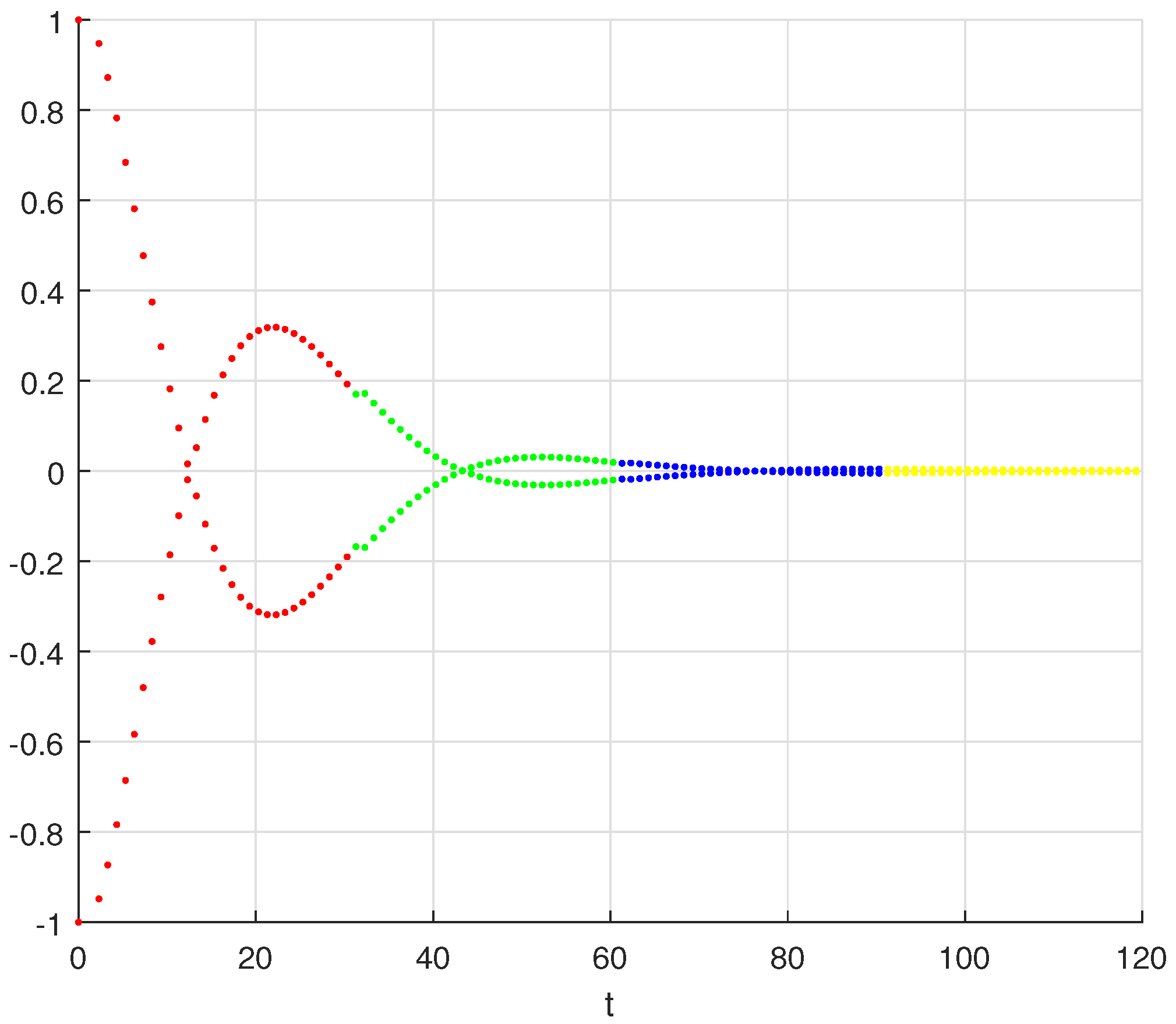
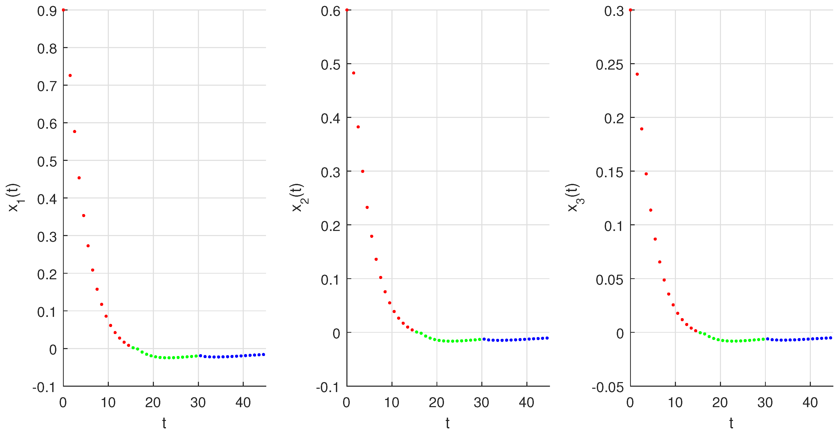
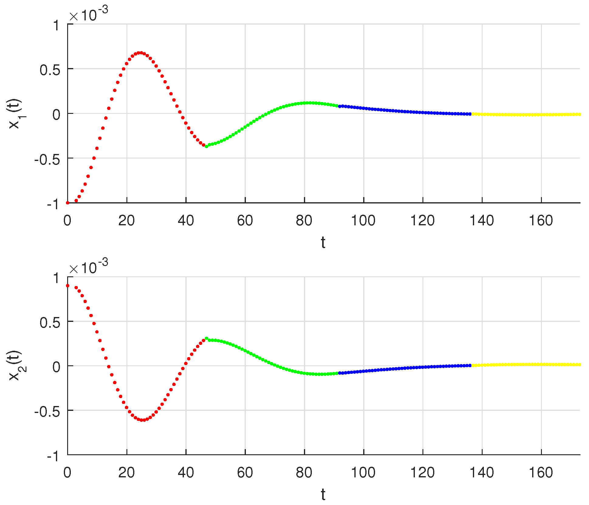
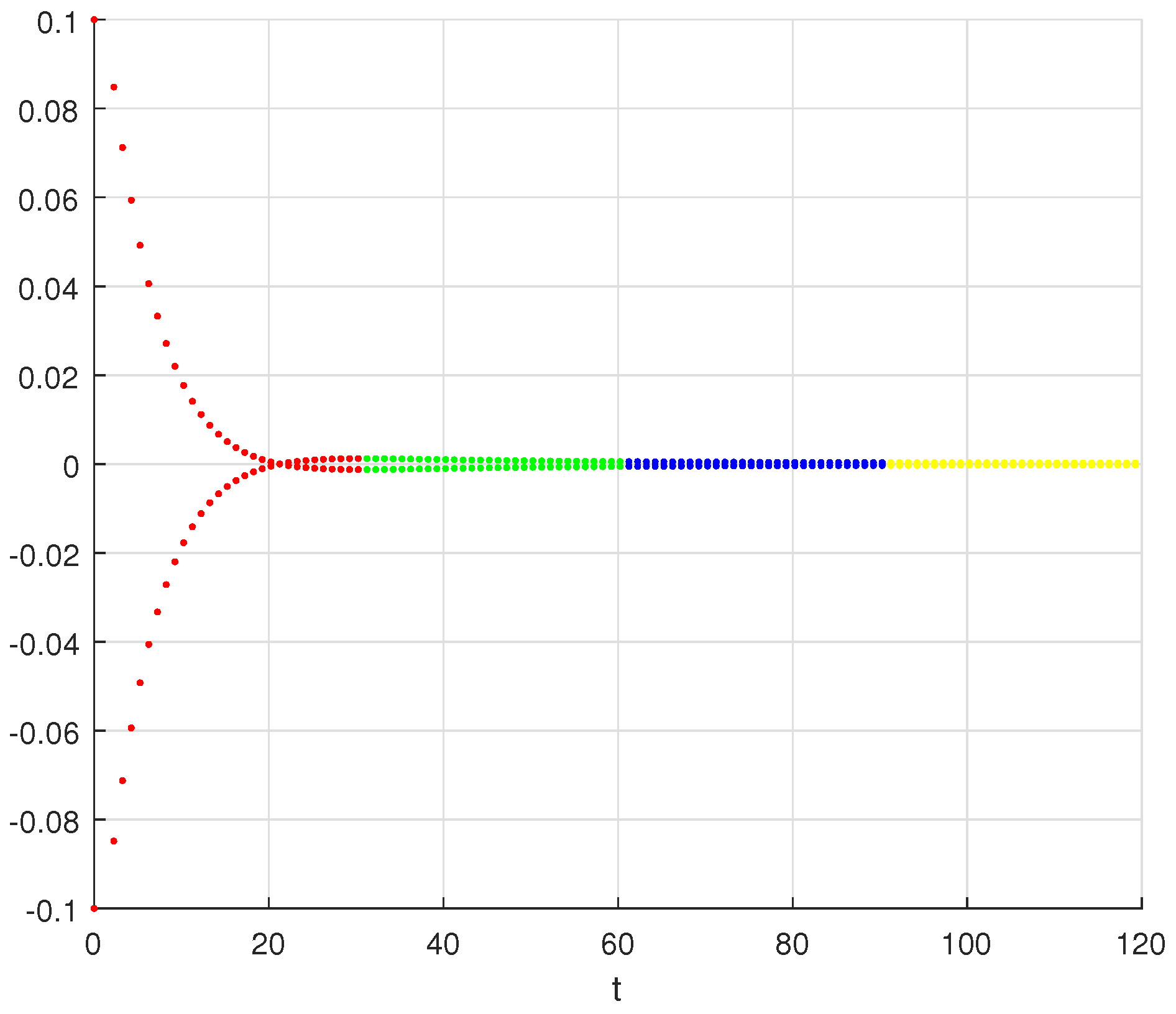
6. Numerical Simulations

Example 1.

Let us consider the following fractional variable-order neural network:

$$\left\{\begin{array}{c}{}_h^C{\Delta }_{t_0}^{v_0}x\left(t\right)=-Ax(t+v_{0}h)+Btanh\left(x(t+v_{0}h)\right),t\in \{t_0+(1-v_0)h,\dots ,t_l-v_{0}h\}\hfill \\ {}_h^C{\Delta }_{t_l}^{v_1}x\left(t\right)=-Ax(t+v_{1}h)+Btanh\left(x(t+v_{1}h)\right),t\in \{t_l+(1-v_l)h,\dots ,t_{2l}-v_{1}h\}\hfill \\ {}_h^C{\Delta }_{t_{2l}}^{v_2}x\left(t\right)=-Ax(t+v_{2}h)+Btanh\left(x(t+v_{2}h)\right),t\in \{t_{2l}+(1-v_2)h,\dots ,t_{3l}-v_{2}h\},\hfill \end{array}\right.$$

(5)

where $h=0.5,$$k=0,1,2,$$t\in {\left(h\mathbb{N}\right)}_{t_{kl}-(1-v_k)h}$ and $(v_0,v_1,v_2)=(0.05,0.1,0.15)$, $tanh\left(x\left(t\right)\right)=(tanh(x_1\left(t\right)),tanh{\left(x_2\left(t\right)\right)}^T)$, and where:

$$A=\left[\begin{array}{c}0.200\\ 00.20\\ 000.2\end{array}\right],B=\left[\begin{array}{c}0.002-0.0040.0015\\ -0.0020.001-0.002\\ -0.00250.0015-0.003\end{array}\right],x\left(0\right)=\left[\begin{array}{c}0.9\\ 0.6\\ 0.3\end{array}\right].$$

We note that the assumptions $\left(A_1\right)$ and $\left(A_2\right)$ are satisfied for $M_A=0.2$ and $M_B=0.0075$. This results in $M=0.9866<1$. Then, the conditions of Theorem 1 are fulfilled for $r\approx 67.16$, which indicates the existence of at least one solution. Theorem 2 is also satisfied for $c={\displaystyle \frac{d}{1-M}}$ where $d=4.7547$, and hence, the system (5) is Ulam–Hyers stable. We use the following numerical formulas to obtain the numerical solution in Figure 1 along with the initial condition $x\left(0\right)={(0.9,0.6,0.3)}^T$, which shows the stability of the considered neural network:

$$\left\{\begin{array}{c}x\left(t\right)=x\left(t_0\right)+{\displaystyle \frac{h^{v_0}}{\Gamma \left(v_0\right)}}\sum _{t_0+1}^t{\displaystyle \frac{\Gamma (t-j+v_0)}{\Gamma (t-j+1)}}\left(-Ax\left(j\right)+Btanh\left(x\right(j\left)\right)\right),\hfill \\ x\left(t\right)=x\left(t_l\right)+{\displaystyle \frac{h^{v_1}}{\Gamma \left(v_1\right)}}\sum _{t_l+1}^t{\displaystyle \frac{\Gamma (t-j+v_0)}{\Gamma (t-j+1)}}\left(-Ax\left(j\right)+Btanh\left(x\right(j\left)\right)\right),\hfill \\ x\left(t\right)=x\left(t_{2l}\right)+{\displaystyle \frac{h^{v_2}}{\Gamma \left(v_2\right)}}\sum _{t_{2l}+1}^t{\displaystyle \frac{\Gamma (t-j+v_0)}{\Gamma (t-j+1)}}\left(-Ax\left(j\right)+Btanh\left(x\right(j\left)\right)\right).\hfill \end{array}\right.$$

Example 2.

Consider the following two-dimensional fractional discrete-time neural network:

$${}_h^C{\Delta }_{t_{kl}}^{v_k}x\left(t\right)=-Ax(t+v_{k}h)+Bsin\left(x(t+v_{k}h)\right),0<v_k\le 1t\in {\left(h\mathbb{N}\right)}_{kl+(1-v_k)h}k=0,1,2,3,$$

(6)

where $sin\left(x\left(t\right)\right)={(sin\left(x_1\left(t\right)\right),sin\left(x_2\left(t\right)\right))}^T$. Suppose $x\left(0\right)={(1,-1)}^T,(v_0,v_1,v_2,v_3)=(0.5,0.4,0.3,0.2),h=1.3$ and $m=4$ and:

$$A=\left[\begin{array}{c}0.0460\\ 00.046\end{array}\right],B=\left[\begin{array}{c}0.00030\\ -0.00040.0002\end{array}\right].$$

We can discuss the stability over different time domains. The parameters satisfy $\left(A_1\right)$ and $\left(A_2\right)$ for $M_A=0.046,$$M_B=0.0006$, and $M=0.9858<1$. All the conditions in Theorem 1 for the existence of the solution are valid with $r\approx 70.42$. Theorem 2 also holds true for the constant $d=21.155$ and $c={\displaystyle \frac{d}{1-M}}$, which guarantees that the discrete-time neural network (6) is Ulam–Hyers stable. The numerical solution of the system is illustrated in Figure 2.

Example 3.

Consider the following neural network:

$$\left\{\begin{array}{c}{}_h^C{\Delta }_{t_{kl}}^{v_k}{x}_1\left(t\right)=-a_1{x}_1(t+v_{k}h)+b_{11}sin\left(x_1(t+v_{k}h)\right)+b_{12}sin\left(x_2(t+v_{k}h)\right),\hfill \\ {}_h^C{\Delta }_{t_{kl}}^{v_k}{x}_2\left(t\right)=-a_2{x}_2(t+v_{1}h)+b_{21}sin\left(x_1(t+v_{k}h)\right)+b_{22}sin\left(x_2(t+v_{k}h)\right),\hfill \end{array}\right.$$

(7)

where $t\in {\left(h\mathbb{N}\right)}_{t_{kl}+(1-v_k)h},m=4$ and $0<v_k\le 1.$ We consider in this example the following two cases:

$\mathbf{Case} 1$

Let $t\in [0,173],h=1.9,(v_0,v_1,v_2,v_3)=(0.8,0.6,0.3,0.4).$ and:

$$A=\left[\begin{array}{c}0.0150\\ 00.015\end{array}\right],B=\left[\begin{array}{c}-0.00030\\ -0.00040.0002\end{array}\right],x\left(0\right)=\left[\begin{array}{c}-0.001\\ 0.0009\end{array}\right].$$

Here, from the given data, we obtain $M_A=0.015$ and $M_B=0.0006$. Clearly, the assumptions ($A_1$) and ($A_2$) hold with $M=0.9212<1$. Thus, all the conditions of Theorem 1 and Theorem 2 are satisfied. Therefore, the system (7) has at least one solution that is Ulam–Hyers stable for $r\approx 0.0127,$$d=59.051$ and $c={\displaystyle \frac{d}{1-M}}$;

$\mathbf{Case} 2$

We admit that $t\in [0,120],h=1.25,(v_0,v_1,v_2,v_3)=(0.05,0.05,0.05,0.05),$ and:

$$A=\left[\begin{array}{c}0.10\\ 00.1\end{array}\right],B=\left[\begin{array}{c}-0.030.02\\ -0.010.06\end{array}\right],x\left(0\right)=\left[\begin{array}{c}-0.1\\ 0.1\end{array}\right].$$

As observed, ($A_1$) and $\left(A_2\right)$ are valid for $M_A=0.1,$$M_B=0.07$, and $M=0.9212$. With $r\approx 1.269$, Theorem 1 is valid, which implies the existence of the solution. We can easily confirm that the neural network (7) is Ulam–Hyers stable, as there is a constant $c={\displaystyle \frac{d}{1-M}}$ where $d=5.419$, and hence, Theorem 2 accurately holds.

The stability is shown in Figure 3 and Figure 4 using the following numerical formulas:

$$\left\{\begin{array}{c}{x}_1\left(t\right)=x_1\left(t_{kl}\right)+{\displaystyle \frac{h^{v_k}}{\Gamma \left(v_k\right)}}\sum _{t_k+1}^i{\displaystyle \frac{\Gamma (t-j+v_k)}{\Gamma (t-j+1)}}\left(-a_1{x}_1\left(j\right)+b_{11}sin\left(x_1\left(j\right)\right)+b_{12}sin\left(x_2\left(j\right)\right)\right)\hfill \\ x_2\left(t\right)=x_2\left(t_{kl}\right)+{\displaystyle \frac{h^{v_k}}{\Gamma \left(v_k\right)}}\sum _{t_k+1}^i{\displaystyle \frac{\Gamma (t-j+v_k)}{\Gamma (t-j+1)}}\left(-a_2{x}_2\left(j\right)+b_{21}sin\left(x_1\left(j\right)\right)+b_{22}sin(x_2\left(j\right)\right).\hfill \end{array}\right.$$

In this paper, we addressed the existence and stability of a novel type of discrete fractional neural network with a variable order. In comparison to the literature that already exists concerning the technique used in our work, Reference [10] provided Ulam–Hyers stability results for Caputo nabla fractional difference equations in both the linear and non-linear cases using the generalized Gronwall inequality, and on the other hand, Reference [11] investigated the Hyers–Ulam stability of a linear fractional neural network with the help of the discrete Laplace transform. Furthermore, the existence of solutions for an initial-value discrete fractional Duffing equation with a forcing term using the Krasnoselskii fixed-point theorem and the Hyers–Ulam stability was shown in [12]. According to the literature reviewed above, it should be noted that the model addressed in this work is far more complex than the ones explored previously, and this type of discrete neural network with the variable-order fractional Caputo h-difference operator has not previously been investigated. As a consequence, when compared to [10,11,12], all of the results and discussions in this work are novel and enhanced.

7. Conclusions

This paper makes a contribution to the topic of the stability of fractional discrete neural networks by presenting a variable-order network model and by proving its Ulam–Hyers stability. Specifically, two novel theorems were proven: one theorem regards the existence of the solution for the proposed variable-order model, whereas the other regards its Ulam–Hyers stability. Finally, numerical simulations were carried out to show the effectiveness of the theoretical approach developed herein.

References

1. Hilfer, R. Applications of Fractional Calculus in Physics; World Scientific: Singapore, 2000. [Google Scholar]
2. Goodrich, C.; Peterson, A.C. Discrete Fractional Calculus; Springer: Berlin/Heidelberg, Germany, 2015. [Google Scholar]
3. Stanisławski, R.; Latawiec, K.J. A modified Mikhailov stability criterion for a class of discrete-time noncommensurate fractional-order systems. Commun. Nonlinear Sci. Numer. Simul. 2021, 96, 105697. [Google Scholar] [CrossRef]
4. Wei, Y.; Wei, Y.; Chen, Y.; Wang, Y. Mittag–Leffler stability of nabla discrete fractional-order dynamic systems. Nonlinear Dyn. 2020, 101, 407–417. [Google Scholar] [CrossRef]
5. Khennaoui, A.-A.; Ouannas, A.; Bendoukha, S.; Grassi, G.; Wang, X.; Pham, V.-T.; Alsaadi, F.E. Chaos, control, and synchronization in some fractional-order difference equations. Adv. Differ. Equ. 2019, 2019, 412. [Google Scholar] [CrossRef] [Green Version]
6. Humphries, U.; Rajchakit, G.; Kaewmesri, P.; Chanthorn, P.; Sriraman, R.; Samidurai, R.; Lim, C.P. Global Stability Analysis of Fractional-Order Quaternion-Valued Bidirectional Associative Memory Neural Networks. Mathematics 2020, 8, 801. [Google Scholar] [CrossRef]
7. Ratchagit, K. Asymptotic stability of delay-difference system of Hopfield neural networks via matrix inequalities and application. Int. J. Neural Syst. 2007, 17, 425–430. [Google Scholar] [CrossRef]
8. Pratap, A.; Raja, R.; Alzabut, J.; Cao, J.; Rajchakit, G.; Huang, C. Mittag–Leffler stability and adaptive impulsive synchronization of fractional order neural networks in quaternion field. Math. Methods Appl. Sci. 2020, 43, 6223–6253. [Google Scholar] [CrossRef]
9. Du, F.; Jia, B. Finite time stability of fractional delay difference systems: A discrete delayed Mittag–Leffler matrix function approach. Chaos Solitons Fractals 2020, 141, 110430. [Google Scholar] [CrossRef]
10. Chen, C.; Bohner, M.; Jia, B. Ulam–Hyers stability of Caputo fractional difference equations. Math. Methods Appl. Sci. 2019, 42, 7461–7470. [Google Scholar] [CrossRef]
11. Jonnalagadda, J.M. Hyers-Ulam stability of fractional nabla difference equations. Int. J. Anal. 2016, 2016, 1–5. [Google Scholar] [CrossRef] [Green Version]
12. Selvam, A.G.M.; Baleanu, D.; Alzabut, J.; Vignesh, D.; Abbas, S. On Hyers–Ulam Mittag–Leffler stability of discrete fractional Duffing equation with application on inverted pendulum. Adv. Differ. Equ. 2020, 2020, 456. [Google Scholar] [CrossRef]
13. Sun, H.; Zhang, Y.; Baleanu, D.; Chen, W.; Chen, Y. A new collection of real world applications of fractional calculus in science and engineering. Commun. Nonlinear Sci. Numer. Simul. 2018, 64, 213–231. [Google Scholar] [CrossRef]
14. Pratap, A.; Raja, R.; Cao, J.; Huang, C.; Niezabitowski, M.; Bagdasar, O. Stability of discrete-time fractional-order time-delayed neural networks in complex field. Math. Methods Appl. Sci. 2021, 44, 419–440. [Google Scholar] [CrossRef]
15. Li, R.; Cao, J.; Xue, C.; Manivannan, R. Quasi-stability and quasi-synchronization control of quaternion-valued fractional-order discrete-time memristive neural networks. Appl. Math. Comput. 2021, 395, 125851. [Google Scholar] [CrossRef]
16. You, X.; Song, Q.; Zhao, Z. Global Mittag–Leffler stability and synchronization of discrete-time fractional-order complex-valued neural networks with time delay. Neural Netw. 2020, 122, 382–394. [Google Scholar] [CrossRef] [PubMed]
17. Gu, Y.; Wang, H.; Yu, Y. Synchronization for fractional-order discrete-time neural networks with time delays. Appl. Math. Comput. 2020, 372, 124995. [Google Scholar] [CrossRef]
18. Wu, G.-C.; Abdeljawad, T.; Liu, J.; Baleanu, D.; Wu, K.-T. Mittag–Leffler Stability Analysis of Fractional Discrete-Time Neural Networks via Fixed Point Technique; Institute of Mathematics and Informatics: Sofia, Bulgaria, 2019. [Google Scholar]
19. You, X.; Dian, S.; Guo, R.; Li, S. Exponential stability analysis for discrete-time quaternion-valued neural networks with leakage delay and discrete time-varying delays. Neurocomputing 2021, 430, 71–81. [Google Scholar] [CrossRef]
20. You, X.; Song, Q.; Zhao, Z. Existence and finite-time stability of discrete fractional-order complex-valued neural networks with time delays. Neural Netw. 2020, 123, 248–260. [Google Scholar] [CrossRef] [PubMed]
21. Huang, L.-L.; Park, J.H.; Wu, G.-C.; Mo, Z.-W. Variable-order fractional discrete-time recurrent neural networks. J. Comput. Appl. Math. 2020, 370, 112633. [Google Scholar] [CrossRef]
22. Baleanu, D.; Wu, G.-C.; Bai, Y.-R.; Chen, F.-L. Stability analysis of Caputo–like discrete fractional systems. Commun. Nonlinear Sci. Numer. Simul. 2017, 48, 520–530. [Google Scholar] [CrossRef]
23. Burton, T.A.; Furumochi, T. Krasnoselskii’s fixed point theorem and stability. Nonlinear Anal. Theory Methods Appl. 2002, 49, 445–454. [Google Scholar] [CrossRef]
Figure 1. Numerical solution of the variable-order neural network (5) (red = 0.05, green = 0.1, blue = 0.15).
Fractalfract 06 00119 g001
Figure 2. The numerical solution of the neural network (6).
Fractalfract 06 00119 g002
Figure 3. Numerical solution of the neural network (7), Case 1.
Fractalfract 06 00119 g003
Figure 4. Neural network (7), Case 2.
Fractalfract 06 00119 g004
Publisher’s Note: MDPI stays neutral with regard to jurisdictional claims in published maps and institutional affiliations.