
Starlike Functions of Complex Order with Respect to Symmetric Points Defined Using Higher Order Derivatives

 ,
,  , , and
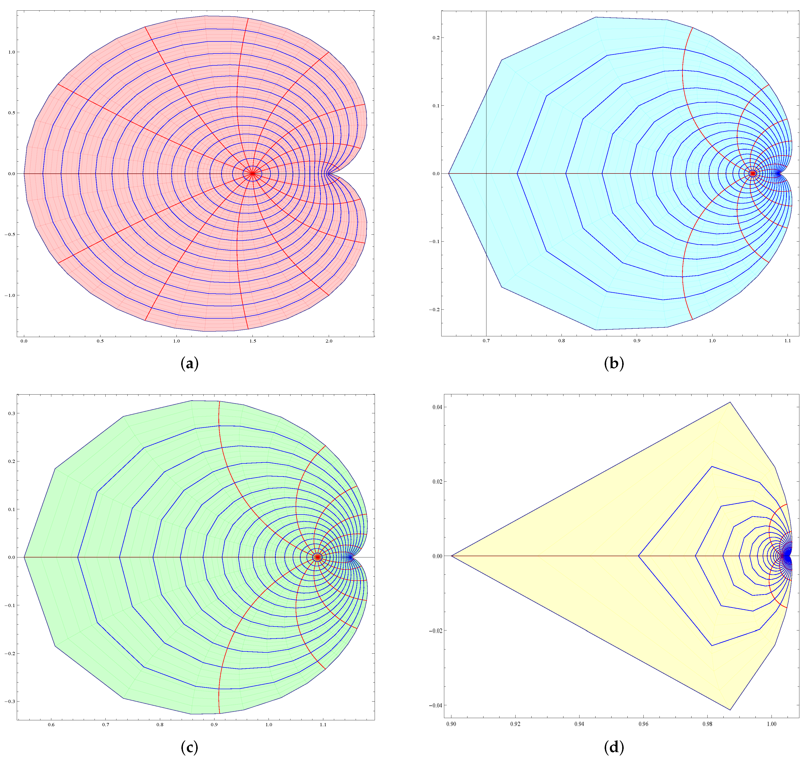
Abstract
1. Introduction and Definitions
1.1. Motivation, Novelty and Discussion
1.2. Comparison on The Impact of on Two Different Conic Regions
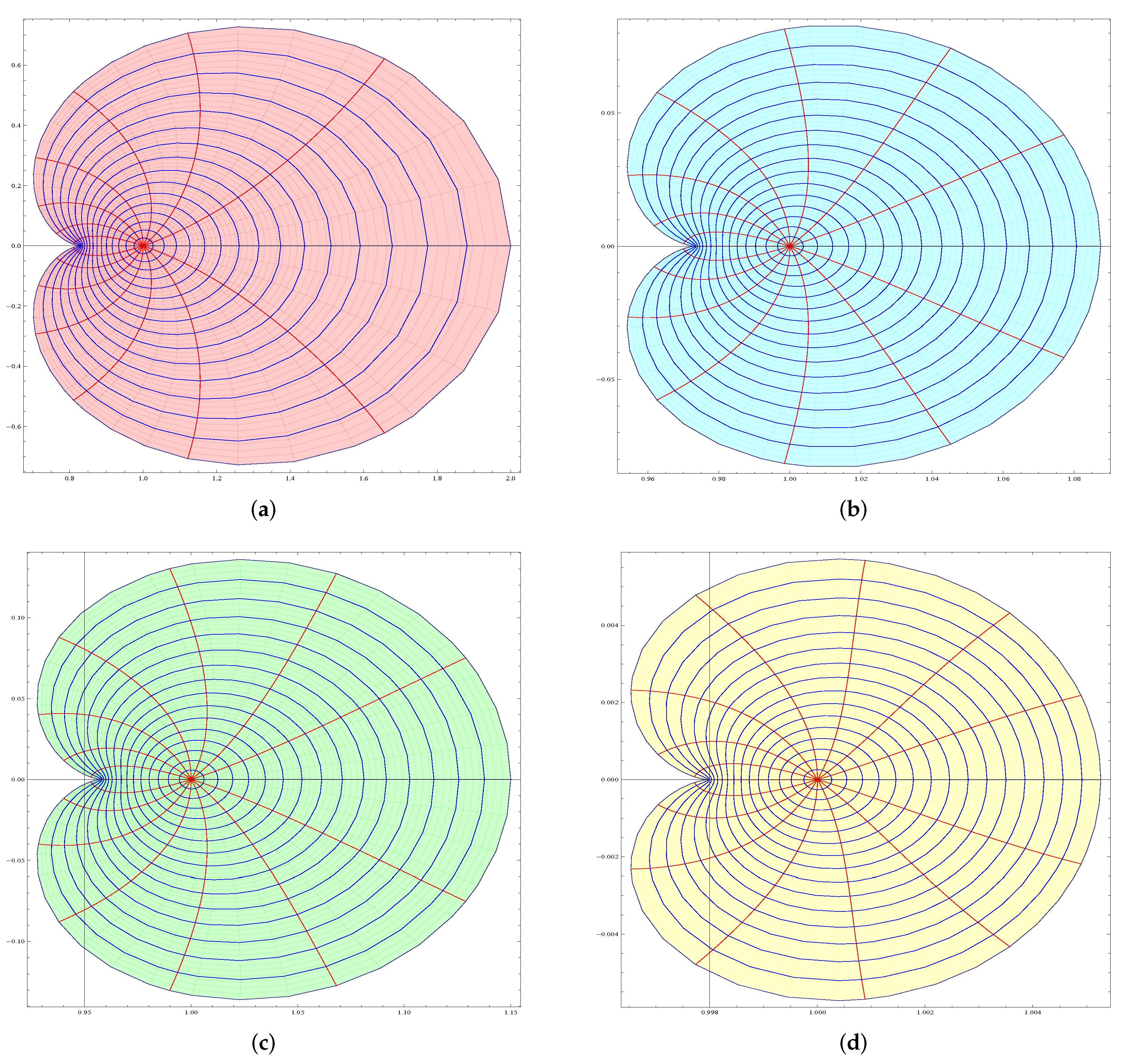
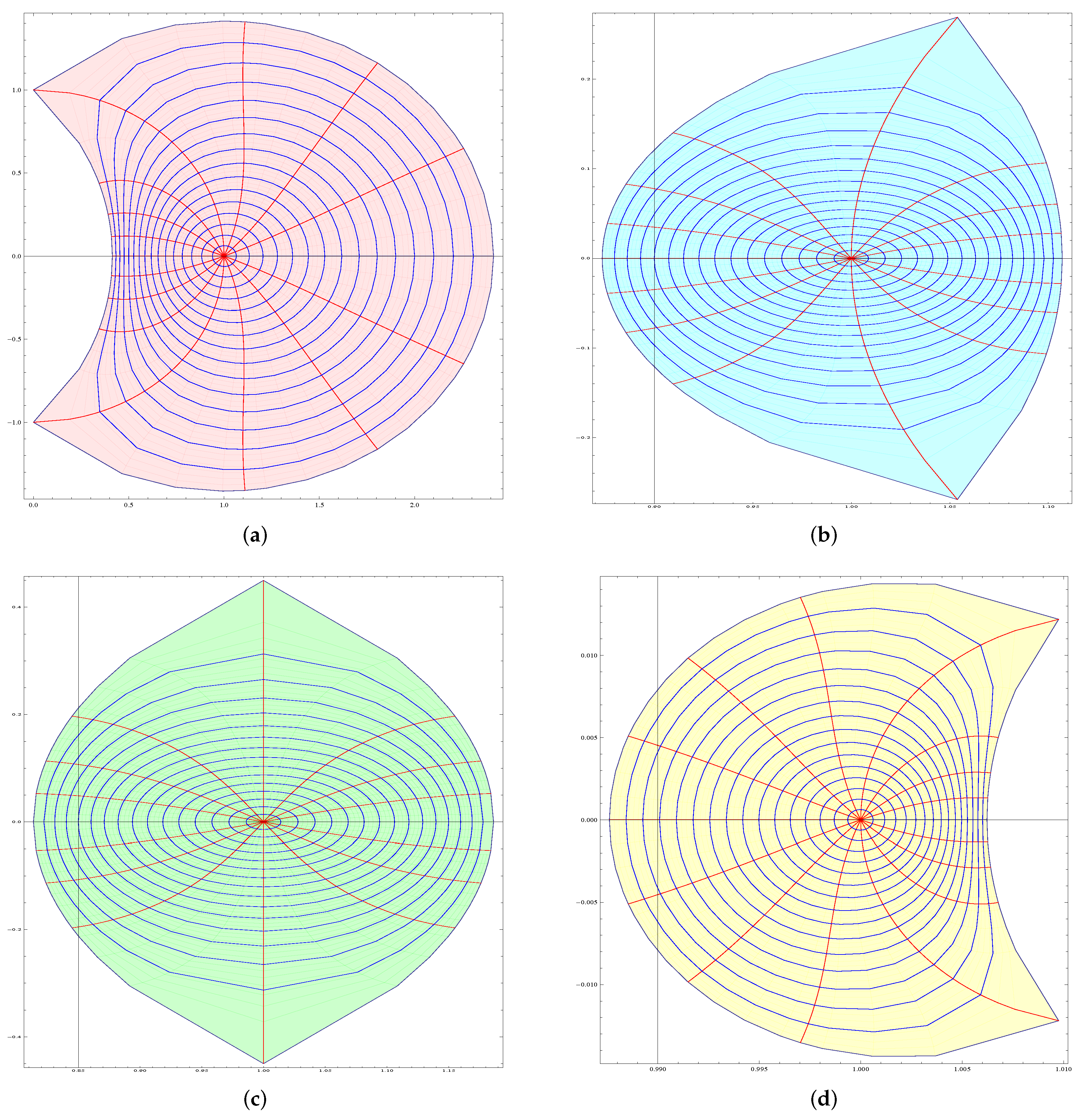
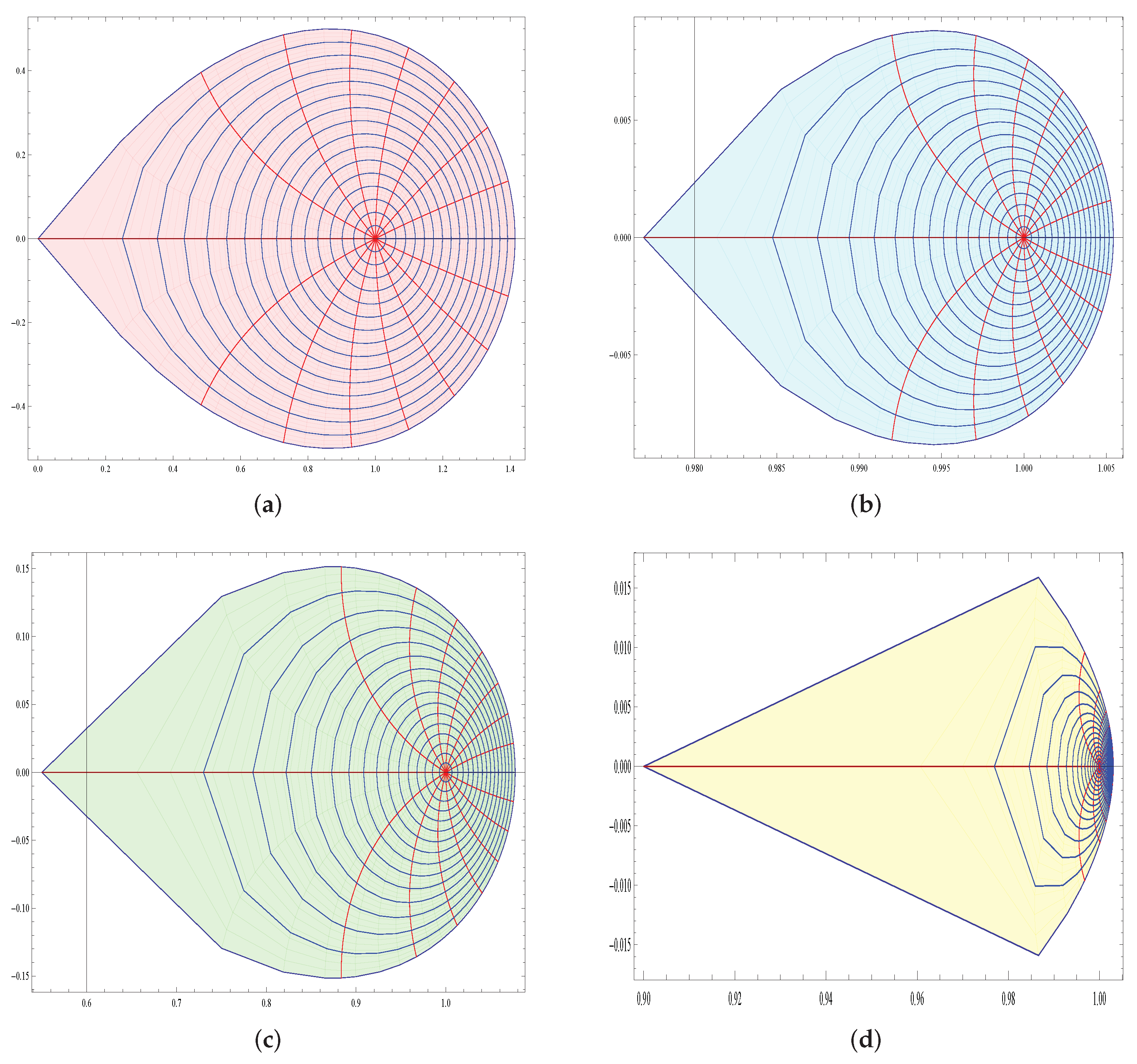
- Cardioid region with cusp on the right hand side, ().
- Cardioid region with cusp on left hand side, .
- It is well-known that is univalent in and maps the unit disc onto the interior of the cardioid with cusp on the right hand side in the right half plane (see Figure 1a). Note that while , it does not have the usual normalization . The impact of on is that the map is circular if F and G are chosen remotely (far off), while the curves are polygonal (see Figure 1d) if F and G are chosen close enough. The presence of is helpful in translation.
- Now, if we choose
- (i)
- (ii)
- If we replace , , and in where is defined as in (5), we can obtain and classes defined by Noor and Malik in [19] (Definition 1.3 and Definition 1.4) by choosing and , respectively.
- (iii)
- If we let , , , and , then reduces to the classes defined by Shanmugam, Ramachandran and Ravichandran [26] (Definition 1.3).
- (iv)
- If we let , , , and , then the class reduces to well-known class Bazilevič function defined by
2. Preliminaries
3. Fekete-Szegö Inequalities for the Class
Some Applications Involving Bernoulli Lemniscate and Shell Shaped Region
4. Subordination Results for Functions with Respect to Symmetric Points
5. Classes of Multivalent Functions Using Quantum Calculus
Main Results Involving Quantum Calculus
6. Conclusions
Author Contributions
Funding
Institutional Review Board Statement
Informed Consent Statement
Data Availability Statement
Acknowledgments
Conflicts of Interest
References
- Goodman, A.W. Univalent Functions; Mariner Publishing Co., Inc.: Tampa, FL, USA, 1983; Volume I. [Google Scholar]
- Hayman, W.K. Multivalent Functions; Cambridge Tracts in Mathematics and Mathematical Physics, No. 48; Cambridge University Press: Cambridge, UK, 1958. [Google Scholar]
- Haji Mohd, M.; Darus, M. Fekete-Szegö problems for quasi-subordination classes. Abstr. Appl. Anal. 2012, 2012, 192956. [Google Scholar] [CrossRef]
- Karthikeyan, K.R.; Murugusundaramoorthy, G.; Cho, N.E. Some inequalities on Bazilevič class of functions involving quasi-subordination. AIMS Math. 2021, 6, 7111–7124. [Google Scholar] [CrossRef]
- Ma, W.C.; Minda, D. A unified treatment of some special classes of univalent functions. In Lecture Notes Analysis, I, Proceedings of the Conference on Complex Analysis, Tianjin, China, 19–23 June 1992; International Press Inc.: Cambridge, MA, USA, 1992; pp. 157–169. [Google Scholar]
- Sokół, J. Coefficient estimates in a class of strongly starlike functions. Kyungpook Math. J. 2009, 49, 349–353. [Google Scholar] [CrossRef]
- Raina, R.K.; Sokół, J. Some properties related to a certain class of starlike functions. C. R. Math. Acad. Sci. Paris 2015, 353, 973–978. [Google Scholar] [CrossRef]
- Raina, R.K.; Sokół, J. Fekete-Szegö problem for some starlike functions related to shell-like curves. Math. Slovaca 2016, 66, 135–140. [Google Scholar] [CrossRef]
- Aouf, M.K.; Dziok, J.; Sokół, J. On a Subclass of Strongly Starlike Functions. Appl. Math. Lett. 2011, 24, 27–32. [Google Scholar] [CrossRef]
- Dziok, J.; Raina, R.K.; Sokół, J. On α-convex functions related to shell-like functions connected with Fibonacci numbers. Appl. Math. Comput. 2011, 218, 996–1002. [Google Scholar] [CrossRef]
- Dziok, J.; Raina, R.K.; Sokół, J. Certain results for a class of convex functions related to a shell-like curve connected with Fibonacci numbers. Comput. Math. Appl. 2011, 61, 2605–2613. [Google Scholar] [CrossRef]
- Dziok, J.; Raina, R.K.; Sokół, J. On a class of starlike functions related to a shell-like curve connected with Fibonacci numbers. Math. Comput. Model. 2013, 57, 1203–1211. [Google Scholar] [CrossRef]
- Gandhi, S.; Ravichandran, V. Starlike functions associated with a lune. Asian-Eur. J. Math. 2017, 10, 1750064. [Google Scholar] [CrossRef]
- Khatter, K.; Ravichandran, V.; Sivaprasad Kumar, S. Starlike functions associated with exponential function and the lemniscate of Bernoulli. Rev. R. Acad. Cienc. Exactas Fís. Nat. Ser. A Mat. RACSAM 2019, 113, 233–253. [Google Scholar] [CrossRef]
- Mendiratta, R.; Nagpal, S.; Ravichandran, V. A subclass of starlike functions associated with left-half of the lemniscate of Bernoulli. Internat. J. Math. 2014, 25, 1450090. [Google Scholar] [CrossRef]
- Janowski, W. Some extremal problems for certain families of analytic functions I. Ann. Polon. Math. 1973, 10, 297–326. [Google Scholar] [CrossRef]
- Aouf, M.K. On a class of p-valent starlike functions of order α. Internat. J. Math. Math. Sci. 1987, 10, 733–744. [Google Scholar] [CrossRef]
- Breaz, D.; Karthikeyan, K.R.; Senguttuvan, A. Multivalent prestarlike functionswith respect to symmetric points. Symmetry 2022, 14, 20. [Google Scholar]
- Noor, K.I.; Malik, S.N. On coefficient inequalities of functions associated with conic domains. Comput. Math. Appl. 2011, 62, 2209–2217. [Google Scholar] [CrossRef]
- Aouf, M.K.; Bulboacă, T.; Seoudy, T.M. Subclasses of multivalent non-Bazilevič functions defined with higher order derivatives. Bull. Transilv. Univ. Braşov Ser. III 2020, 13, 411–422. [Google Scholar] [CrossRef]
- Karthikeyan, K.R.; Murugusundaramoorthy, G.; Bulboacă, T. Properties of λ-pseudo-starlike functions of complex order defined by subordination. Axioms 2021, 10, 86. [Google Scholar] [CrossRef]
- Ahuja, O.; Bohra, N.; Cetinkaya, A.; Kumar, S. Univalent functions associated with the symmetric points and cardioid-shaped domain involving (p,q)-calculus. Kyungpook Math. J. 2021, 61, 75–98. [Google Scholar]
- Tang, H.; Karthikeyan, K.R.; Murugusundaramoorthy, G. Certain subclass of analytic functions with respect to symmetric points associated with conic region. AIMS Math. 2021, 6, 12863–12877. [Google Scholar] [CrossRef]
- Arif, M.; Wang, Z.-G.; Khan, M.R.; Lee, S.K. Coefficient inequalities for janowski-sakaguchi type functions associated with conic regions. Hacet. J. Math. Stat. 2018, 47, 261–271. [Google Scholar] [CrossRef]
- Arif, M.; Ahmad, K.; Liu, J.-L.; Sokół, J. A new class of analytic functions associated with Sălăgean operator. J. Funct. Spaces 2019, 8, 6157394. [Google Scholar] [CrossRef]
- Shanmugam, T.N.; Ramachandran, C.; Ravichandran, V. Fekete-Szegö problem for subclasses of starlike functions with respect to symmetric points. Bull. Korean Math. Soc. 2006, 43, 589–598. [Google Scholar] [CrossRef]
- Ibrahim, R.W. On a Janowski formula based on a generalized differential operator. Commun. Fac. Sci. Univ. Ank. Ser. A1 Math. Stat. 2020, 69, 1320–1328. [Google Scholar]
- Kavitha, D.; Dhanalakshmi, K. Subclasses of analytic functions with respect to symmetric and conjugate points bounded by conical domain. Adv. Math. Sci. J. 2020, 9, 397–404. [Google Scholar] [CrossRef]
- Mohankumar, D.; Senguttuvan, A.; Karthikeyan, K.R.; Ganapathy Raman, R. Initial coefficient bounds and Fekete-Szegö problem of pseudo-Bazilevič functions involving quasi-subordination. Adv. Dyn. Syst. Appl. 2021, 16, 767–777. [Google Scholar]
- Mashwan, W.K.; Ahmad, B.; Khan, M.G.; Mustafa, S.; Arjika, S.; Khan, B. Pascu-Type analytic functions by using Mittag-Leffler functions in Janowski domain. Math. Probl. Eng. 2021, 2021, 1209871. [Google Scholar] [CrossRef]
- Raina, R.K.; Sokół, J. On a class of analytic functions governed by subordination. Acta Univ. Sapientiae Math. 2019, 11, 144–155. [Google Scholar] [CrossRef]
- Raina, R.K.; Sokół, J. On coefficient estimates for a certain class of starlike functions. Haceppt. J. Math. Stat. 2015, 44, 1427–1433. [Google Scholar] [CrossRef]
- Sokół, J.; Thomas, D.K. Further results on a class of starlike functions related to the Bernoulli lemniscate. Houst. J. Math. 2018, 44, 83–95. [Google Scholar]
- Pommerenke, C. Univalent Functions; Vandenhoeck & Ruprecht: Göttingen, Germany, 1975; p. 376. [Google Scholar]
- Hallenbeck, D.J.; Ruscheweyh, S. Subordination by convex functions. Proc. Amer. Math. Soc. 1975, 52, 191–195. [Google Scholar] [CrossRef]
- Breaz, D.; Cotîrlǎ, L.-I. The study of the new classes of m-Fold symmetric bi-univalent functions. Mathematics 2022, 10, 75. [Google Scholar] [CrossRef]
- Oros, G.I.; Cotîrlǎ, L.-I. Coefficient estimates and the Fekete–Szegö problem for new classes of m-fold symmetric bi-univalent functions. Mathematics 2022, 10, 129. [Google Scholar] [CrossRef]
- Srivastava, H.M.; Kamalı, M.; Urdaletova, A. A study of the Fekete-Szegö functional and coefficient estimates for subclasses of analytic functions satisfying a certain subordination condition and associated with the Gegenbauer polynomials. AIMS Math. 2022, 7, 2568–2584. [Google Scholar] [CrossRef]
- Murugusundaramoorthy, G.; Bulboacă, T. Hankel determinants for new subclasses of analytic functions related to a shell shaped region. Mathematics 2020, 8, 1041. [Google Scholar] [CrossRef]
- Ibrahim, R.W.; Baleanu, D. Analytic solution of the Langevin differential equations dominated by a multibrot fractal set. Fractal Fract. 2021, 5, 50. [Google Scholar] [CrossRef]
- Ibrahim, R.W.; Baleanu, D. On quantum hybrid fractional conformable differential and integral operators in a complex domain. Rev. Real Acad. Cienc. Exactas Fís. Natur. Ser. A Mat. (RACSAM) 2021, 31, 115. [Google Scholar] [CrossRef]
- Goyal, S.P.; Goswami, P. On sufficient conditions for analytic functions to be Bazilevič. Complex Var. Elliptic Equ. 2009, 54, 485–492. [Google Scholar] [CrossRef]
- Srivastava, H.M. Univalent functions, fractional calculus, and associated generalized hypergeometric functions. In Univalent Functions, Fractional Calculus, and Their Applications (Ko¯riyama, 1988); Ellis Horwood Series Mathematics Applied; Horwood: Chichester, UK, 1988; pp. 329–354. [Google Scholar]
- Ismail, M.E.H.; Merkes, E.; Styer, D. A generalization of starlike functions. Complex Variables Theory Appl. 1990, 14, 77–84. [Google Scholar] [CrossRef]
- Srivastava, H.M. Operators of basic (or q-) calculus and fractional q-calculus and their applications in geometric function theory of complex analysis. Iran. J. Sci. Technol. Trans. A Sci. 2020, 44, 327–344. [Google Scholar] [CrossRef]
- Jackson, F.H. On q-definite integrals. Quart. J. Pure Appl. Math. 1910, 41, 193–203. [Google Scholar]
- Srivastava, H.M.; Khan, B.; Khan, N.; Ahmad, Q.Z. Coefficient inequalities for q-starlike functions associated with the Janowski functions. Hokkaido Math. J. 2019, 48, 407–425. [Google Scholar] [CrossRef]
- Srivastava, H.M.; Ahmad, Q.Z.; Khan, N.; Khan, N.; Khan, B. Hankel and Toeplitz determinants for a subclass of q-starlike functions associated with a general conic domain. Mathematics 2019, 7, 181. [Google Scholar] [CrossRef]
- Srivastava, H.M.; Khan, B.; Khan, N.; Ahmad, Q.Z.; Tahir, M. A generalized conic domain and its applications to certain subclasses of analytic functions. Rocky Mountain J. Math. 2019, 49, 2325–2346. [Google Scholar] [CrossRef]
- Srivastava, H.M.; Khan, N.; Darus, M.; Rahim, M.T.; Ahmad, Q.Z.; Zeb, Y. Properties of spiral-like close-to-convex functions associated with conic domains. Mathematics 2019, 7, 706. [Google Scholar] [CrossRef]
- Srivastava, H.M.; Raza, N.; AbuJarad, E.S.A.; Srivastava, G.; AbuJarad, M.H. Fekete-Szegö inequality for classes of (p, q)-starlike and (p, q)-convex functions. Rev. Real Acad. Cienc. Exactas Fís. Natur. Ser. A Mat. (RACSAM) 2019, 113, 3563–3584. [Google Scholar] [CrossRef]
- Srivastava, H.M.; Tahir, M.; Khan, B.; Ahmad, Q.Z.; Khan, N. Some general classes of q-starlike functions associated with the Janowski functions. Symmetry 2019, 11, 292. [Google Scholar] [CrossRef]
- Srivastava, H.M.; Tahir, M.; Khan, B.; Ahmad, Q.Z.; Khan, N. Some general families of q-starlike functions associated with the Janowski functions. Filomat 2019, 33, 2613–2626. [Google Scholar] [CrossRef]
- Srivastava, H.M.; Khan, N.; Khan, S.; Ahmad, Q.Z.; Khan, B. A class of k-symmetric harmonic functions involving a certain q-derivative operator. Mathematics 2021, 9, 1812. [Google Scholar] [CrossRef]
- Aldawish, I.; Ibrahim, R.W. Solvability of a new q-differential equation related to q-differential inequality of a special type of analytic functions. Fractal Fract. 2021, 5, 228. [Google Scholar] [CrossRef]
- Zhou, H.; Selvakumaran, K.A.; Sivasubramanian, S.; Purohit, S.D.; Tang, H. Subordination problems for a new class of Bazilevič functions associated with k-symmetric points and fractional q-calculus operators. AIMS Math. 2021, 6, 8642–8653. [Google Scholar] [CrossRef]
- Ramachandran, C.; Kavitha, D.; Soupramanien, T. Certain bound for q-starlike and q-convex functions with respect to symmetric points. Int. J. Math. Math. Sci. 2015, 2015, 205682. [Google Scholar] [CrossRef]


Publisher’s Note: MDPI stays neutral with regard to jurisdictional claims in published maps and institutional affiliations. |
© 2022 by the authors. Licensee MDPI, Basel, Switzerland. This article is an open access article distributed under the terms and conditions of the Creative Commons Attribution (CC BY) license (https://creativecommons.org/licenses/by/4.0/).
Share and Cite
Karthikeyan, K.R.; Lakshmi, S.; Varadharajan, S.; Mohankumar, D.; Umadevi, E. Starlike Functions of Complex Order with Respect to Symmetric Points Defined Using Higher Order Derivatives. Fractal Fract. 2022, 6, 116. https://doi.org/10.3390/fractalfract6020116
Karthikeyan KR, Lakshmi S, Varadharajan S, Mohankumar D, Umadevi E. Starlike Functions of Complex Order with Respect to Symmetric Points Defined Using Higher Order Derivatives. Fractal and Fractional. 2022; 6(2):116. https://doi.org/10.3390/fractalfract6020116
Chicago/Turabian StyleKarthikeyan, Kadhavoor R., Sakkarai Lakshmi, Seetharam Varadharajan, Dharmaraj Mohankumar, and Elangho Umadevi. 2022. "Starlike Functions of Complex Order with Respect to Symmetric Points Defined Using Higher Order Derivatives" Fractal and Fractional 6, no. 2: 116. https://doi.org/10.3390/fractalfract6020116
APA StyleKarthikeyan, K. R., Lakshmi, S., Varadharajan, S., Mohankumar, D., & Umadevi, E. (2022). Starlike Functions of Complex Order with Respect to Symmetric Points Defined Using Higher Order Derivatives. Fractal and Fractional, 6(2), 116. https://doi.org/10.3390/fractalfract6020116