Article

A Robust Controller of a Reactor Electromicrobial System Based on a Structured Fractional Transformation for Renewable Energy

by
Muhammad Zia Ur Rahman
1,2,*,
Rabia Liaquat
3,
Mohsin Rizwan
2,
Carlos Martin-Barreiro
4,5 and
Víctor Leiva
6,*
1
Department of Mechanical, Mechatronics and Manufacturing Engineering, University of Engineering and Technology Lahore, Faisalabad Campus, Faisalabad 38000, Pakistan
2
Department of Mechatronics and Control Engineering, University of Engineering and Technology Lahore, Lahore 54890, Pakistan
3
U.S.-Pakistan Centre for Advanced Studies in Energy, National University of Sciences and Technology, Islamabad 44000, Pakistan
4
Faculty of Natural Sciences and Mathematics, Escuela Superior Politécnica del Litoral ESPOL, Guayaquil 090902, Ecuador
5
Faculty of Engineering, Universidad Espíritu Santo, Samborondón 0901952, Ecuador
6
School of Industrial Engineering, Pontificia Universidad Católica de Valparaíso, Valparaíso 2362807, Chile
*
Authors to whom correspondence should be addressed.
Fractal Fract. 2022, 6(12), 736; https://doi.org/10.3390/fractalfract6120736
Submission received: 14 November 2022 / Revised: 2 December 2022 / Accepted: 6 December 2022 / Published: 12 December 2022
(This article belongs to the Special Issue Fractional Order Controllers: Design and Applications)

Abstract

:
The focus on renewable energy is increasing globally to lessen reliance on conventional sources and fossil fuels. For renewable energy systems to work at their best and produce the desired results, precise feedback control is required. Microbial electrochemical cells (MEC) are a relatively new technology for renewable energy. In this study, we design and implement a model-based robust controller for a continuous MEC reactor. We compare its performance with those of traditional methods involving a proportional integral derivative (PID), H-infinity (H ) controller and PID controller tuned by intelligent genetic algorithms. Recently, a dynamic model of a MEC continuous reactor was proposed, which describes the complex dynamics of MEC through a set of nonlinear differential equations. Until now, no model-based control approaches for MEC have been proposed. For optimal and robust output control of a continuous-reactor MEC system, we linearize the model to state a linear time-invariant (LTI) state-space representation at the nominal operating point. The LTI model is used to design four different types of controllers. The designed controllers and systems are simulated, and their performances are evaluated and compared for various operating conditions. Our findings show that a structured linear fractional transformation (LFT)-based H control approach is much better than the other approaches against various performance parameters. The study provides numerous possibilities for control applications of continuous MEC reactor processes.

1. Introduction

The study of renewable energy is now a worldwide priority [1,2]. Wind, biomass, and solar-based domains are the most common and offer viable sources of renewable energy [3]. Even though wind and solar energies are reliable and promising renewable sources, they depend heavily on weather conditions. Microbial electrochemical cells (MEC) are a technology related to microbial fuel cells (MFC) [4] and a new biomass-based source of renewable energy. While MFC produces an electric current from the microbial decomposition of organic compounds, MEC partially reverse the process to obtain hydrogen or methane from organic material by applying such a current [4].
Global warming is a serious issue worldwide, and fossil fuel consumption is one of its major contributors. Therefore, it is essential to minimize reliance on this type of fuel [5,6] and adopt alternatives with fewer emissions. The greenhouse effects are also reduced by using clean energy. The hydrogen or methane obtained from MEC may be employed to generate electricity throughout an internal combustion engine as an alternative to fossil fuels [7]. Presently, hydrogen is regarded as the most energetic element per unit weight and a clean, renewable energy source with negligible emissions [8,9].
The MEC systems are based on two parts: (i) microorganisms, which adhere to the anode; and (ii) materials—that is, the anode in MEC can be the same as in MFC and often related to carbon and graphite. Platinum may be utilized as a catalyst to reduce the overpotential needed for hydrogen production. However, the high cost of platinum is driving research into biocathodes as an alternative [10].
The generation of renewable energy in MEC processes employs wastewater, food scraps, and synthetic industrial effluent as substrates [11,12], which are the input to the anodic chamber of the continuous MEC. The organic elements in the input substrate are oxidized using low external voltage and an anaerobic microbial population in the anodic compartment of MEC [13]. Microorganisms produce electrons and protons while digesting the organic contents in wastewater in the anodic compartment. To create renewable hydrogen using a reduction process of electrons and protons, the electrons go through an external circuit, and protons move through the membrane to the cathodic chamber [14,15]. Note that current and hydrogen directly connect the MEC process and then the hydrogen production is regulated by adjusting the MEC current.
The research on MEC systems is divided into two areas: (a) material-based analysis for hydrogen generation, and (b) mathematical modeling and process control of such systems. One of the main challenges in designing MEC systems is to control the system inputs and parameters to obtain a constant hydrogen generation rate. When creating systems in real time, modeling, process control, stabilization, and simulations are crucial factors [16,17,18].
The primary role of feedback control [19] in biochemical MEC processes is to create the desired output. The MFC technology received much attention recently, with many dynamic models being proposed [20,21,22,23]. Researchers developed control-oriented models for process implementations in MFC [24,25]. Nonetheless, there is a dearth of research on mathematical modeling and control of relatively new MEC systems. Our critical bibliographical review and a recent study on MEC modeling demonstrate the lack of control-oriented formulation and model-based standard controls for MEC systems [26,27].
The feedback control of MEC systems for regulated hydrogen production has received very little research [26]. Optimal control methods and traditional proportional integral derivative (PID) control strategies for fed-batch MEC systems were discussed [28,29]. Nevertheless, to the best of our knowledge, advanced control methods of model-based robust optimal design for continuous MEC systems have never been studied until now. A minimal amount of literature is available on conventional control of continuous MEC systems based on algebraic manipulations of nonlinear dynamics in continuous MEC processes [30]. Model-based feedback-robust control is necessary for the optimal output of this recently developed renewable energy MEC system.
A dynamic model for MEC systems was proposed in [31]. However, no control schemes have been stated for this model until now. Note that feedback control of these systems can produce the desired output. The linear model-based controllers are helpful because they are easy to be implemented. A model in the state-space form to be linearized at nominal operating conditions can be used for designing linear and robust controllers.
Four control schemes can be designed for continuous-reactor MEC process. Two schemes are conventional and frequently used in the literature. These schemes are conventional PID and unstructured LFT-based H-infinity (often denoted as H ) controllers. Another developed intelligent MEC process control is the PID controller tuned by genetic algorithms (GA). A fourth controller for the continuous-reactor MEC process is a fixed-structured, LFT-based H controller. Therefore, new linear, time-invariant (LTI) model-based controllers of a continuous reactor based on MEC systems can be proposed.
Frequency domain-based H control techniques are often utilized to synthesize controllers and reach stabilization for a guaranteed performance; some works published on the thematic are presented in [32,33,34,35,36]. Although these robust control systems beat traditional PID controllers in terms of performance, they are limited by the complexity of their architecture. Modifying the loop/complementary sensitivities and calibrating the weight-based high-order synthesis make the conventional H controllers complex.
The real-time usages of conventional robust H controllers in the industry have diminished due to their expensive and sophisticated hardware structures. In addition, PID controllers based on evolutionary algorithms have outstanding performance, but they are computationally expensive [37]. These limitations are relaxed by employing fixed-structure robust control [38].
We suggest an approach that optimizes its controller parameters via fractional transformation-based non-smooth H optimization. One can use a fixed-structure LFT-based H controller to eliminate nonlinearity-related fluctuations in the performance metrics, such as overshoot, steady-state error, and settling time in the transient response. Considering the advantages mentioned above, researchers have used fixed-structure H controllers for several systems [32,39,40].
In summary, to the best of our knowledge, advanced H control methods of model-based robust optimal design for continuous MEC systems are unavailable in the literature. Therefore, the objective of the present investigation is to design and implement a control method for an emerging renewable MEC system. We implement our methodology in the MATLAB software with the help of SIMULINK and the robust control toolbox (RCT), a fast and reliable approach that is used to compute the optimal values of the tunable parameters of the proposed controller. This approach minimizes the H norm to produce a robust and quick transient response of the system [41].
The remainder of this article is structured as follows. The mathematical modeling of the continuous MEC process is introduced in Section 2. This section also includes the dynamic study of the open-loop system and the LTI model created by the system identification toolbox in MATLAB. The proposed fixed-structure H , traditional H , GA-PID, and traditional PID controllers are discussed in Section 3. Section 4 presents the simulation results with a discussion and comparison with other methods, clearly demonstrating the suggested strategy viability. The conclusions are also presented in this section.

2. Mathematical Modeling

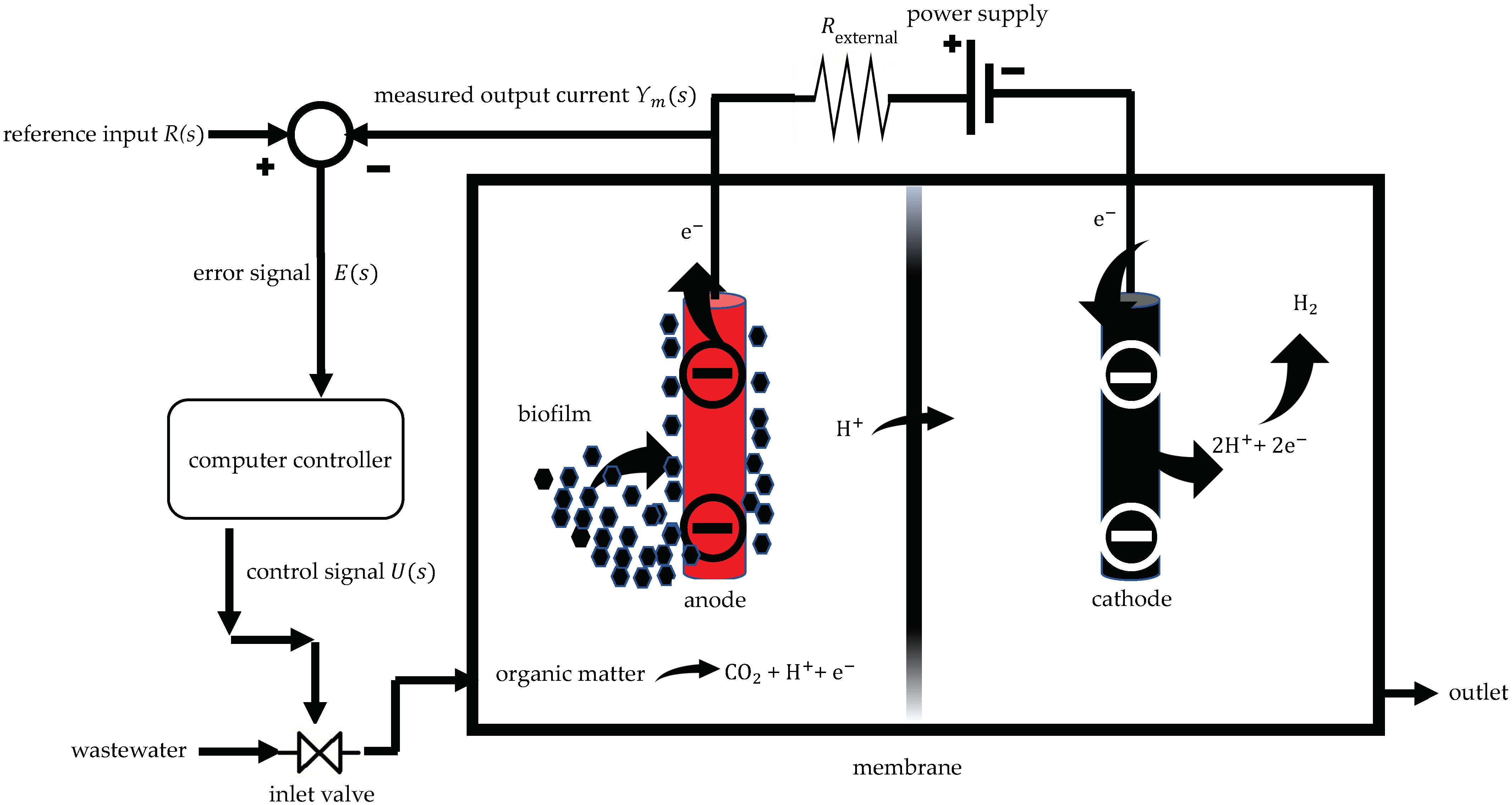
2.1. Description of a Continuous MEC Process

The model suggested in [31] comprises a series of nonlinear ordinary differential equations to describe the dynamical behavior of a continuous MEC process. The foundation of each ordinary differential equation is linked to the steady-state mass balances of the parts of the continuous MEC system. To give the flow of electrons through an external path, the anode is connected to the positive terminal of the direct current (DC) source via an external resistance ( R external ) to be used when measuring MEC current across it and when the system is implemented in real-time. In addition, the cathode is linked to the negative end of the DC source. The model considers the presence of two microbiological occupants in the anode chamber:
(i)
Acetolactic methanogenic;
(ii)
Anodophilic microorganisms.
In Table 1, we can see the assumptions are made in order to model the system’s dynamics.
A continuous MEC system with two chambers—anodic and cathodic—separated by a conductive membrane is shown in Figure 1.
Considering a molecule of acetic acid for the carbon source [42], the chemical processes at a node are stated as
CH 3 COOH + 2 H 2 O + 4 M ox 4 M red + 2 CO 2 4 M red 4 M ox + 8 e + 8 H + CH 3 COOH CH 4 + CO 2 ,
where M ox is an oxidized intracellular mediator, M red is a reduced intracellular mediator, and e is an electron.
The reaction at the cathode is given by
2 H 2 O + 2 e 2 OH + H 2 S .
The dynamic mass balance equations for the substrate ( S ) , anodophilic bacteria ( X a ), and acetoclastic methanogenic bacteria ( X m ) concentrations in the continuous MEC reactor process are presented as
d S ( t ) d t = k a μ a ( t ) X a ( t ) k m μ m ( t ) X m ( t ) + D ( t ) S in S ( t )
d X a ( t ) d t = μ a ( t ) X a ( t ) k d , a X a ( t ) α a D ( t ) X a ( t )
d X m ( t ) d t = μ m ( t ) X m ( t ) k d , m X m ( t ) α m D ( t ) X m ( t ) ,
where, for the time t, S ( t ) is the substrate concentration [ mg S L 1 ] ; X a ( t ) is the anodophilic bacteria concentration [ mgXL 1 ] ; X m ( t ) is the acetoclastic methanogenic bacteria concentration [ mg X L 1 ] ; D ( t ) = F in V reac 1 is the dilution rate [ d 1 ] ; F in is the substrate (wastewater) input flow [ L d 1 ] ; V reac is the reactor volume [L]; μ a is the growth rate for anodophilic bacteria [ d 1 ] ; μ m is the growth rate for acetoclastic methanogenic bacteria [ d 1 ] ; k a is the yield factor for substrate utilization by anodophilic microorganisms in the anode [ mg S mgX 1 ] ; k m is the yield factor for substrate utilization by acetoclastic methanogenic bacteria in the anode [ mg S mg X 1 ] ; k d , a is the anodophilic decay rate [ d 1 ] ; and k d , m is the acetoclastic methanogenic decay rate [ d 1 ] . The kinetic growth rates are defined as [21]
μ a ( t ) = μ max , a S ( t ) ( K S , a + S ( t ) ) 1 ( 1 + exp ( F η / ( R T ) ) )
μ m ( t ) = μ max , m S ( t ) K S , m + S ( t ) ,
where μ max is the maximum growth rate [d 1 ]; K S is the monod half-rate constant; F is the Faraday constant [ C mole 1 ] ; R is the gas constant [ J molK 1 ] ; T is the temperature; and η is the potential difference between anode and cathode [ V ] .
The MEC current density and hydrogen/methane production rates [21,42] are given, respectively, by
I mec ( t ) = ( γ S k a μ a ( t ) X a ( t ) L f 1 f S 0 + γ X b X a ( t ) L f ) V reac Q H 2 ( t ) = Y H 2 A a I mec ( t ) m F R T P Q CH 4 ( t ) = Y CH 4 k m μ m ( t ) X m ( t ) V reac ,
where the yield coefficients, γ X [ mF / MW X ] and γ S [ mF / MW S ], are correlated with the number of coulombs that can be extracted from the biomass and substrate, respectively; f S 0 is the electron dimensionless fraction; b is the endogenous decay factor; L f is the biofilm thickness [m]; Y H 2 is the cathode efficiency; and Y CH 4 is the methane yield.

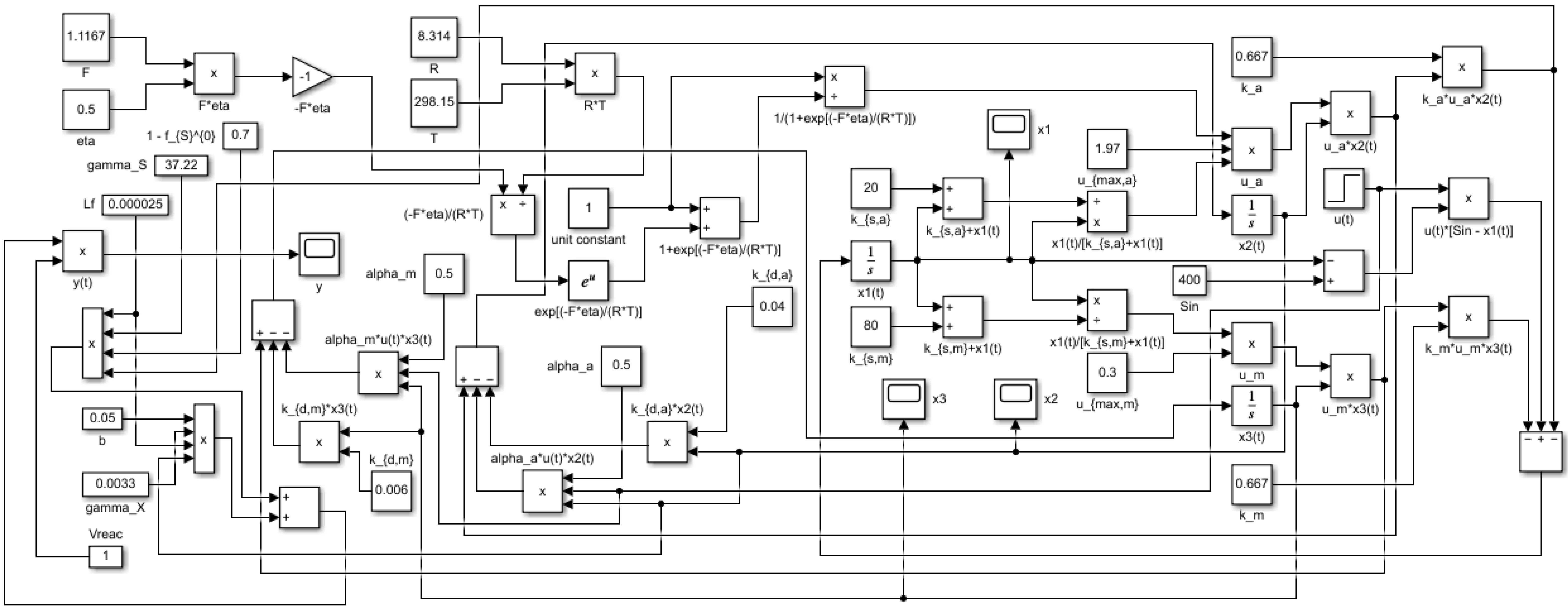
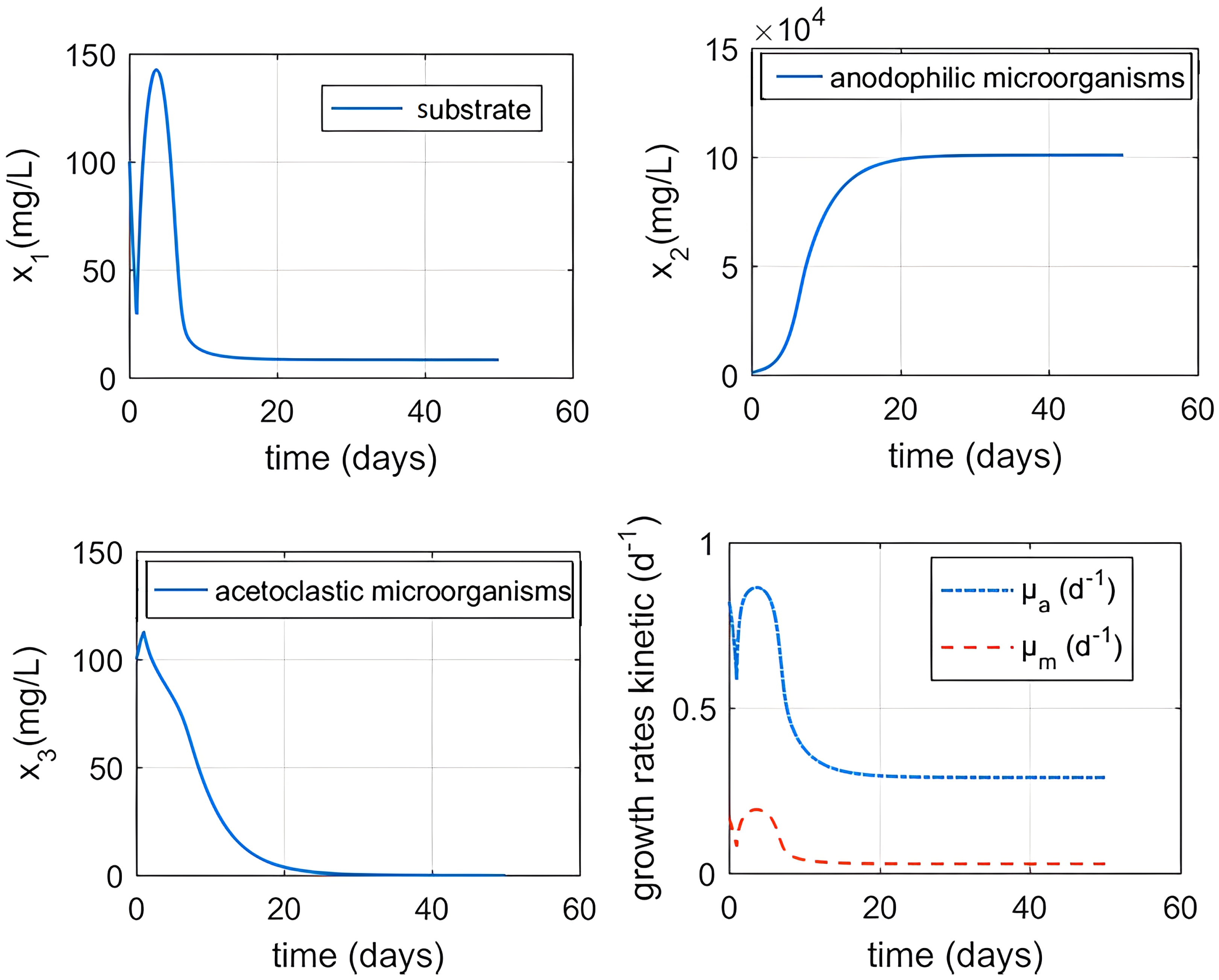
2.2. State-Space Model

From the expressions given in (1)–(6), the system is represented into state-space form as
x ˙ 1 ( t ) = k a μ max , a x 1 ( t ) K S , a + x 1 ( t ) 1 1 + exp ( F R T η ) x 2 ( t ) k m μ max , m x 1 ( t ) K S , m + x 1 ( t ) x 3 ( t ) + u ( t ) ( S in x 1 ( t ) )
x ˙ 2 ( t ) = μ max , a x 1 ( t ) K S , a + x 1 ( t ) 1 1 + exp ( F R T η ) x 2 ( t ) k d , a x 2 ( t ) α a u ( t ) x 2 ( t ) x ˙ 3 ( t ) = μ max , m x 1 ( t ) K S , m + x 1 ( t ) x 3 ( t ) k d , m x 3 ( t ) α m u ( t ) x 3 ( t ) y ( t ) = γ S k a μ max , a x 1 ( t ) K S , a + x 1 ( t ) 1 1 + exp ( F R T η ) x 2 ( t ) L f 1 f S 0 + γ X b x 2 ( t ) L f V reac .
In Table 2, we can see the dependent variables of (7). The state-space model considers the nominal parameter values [31,42]. The complete description and nominal values of parameters are given in Table 3. Figure 2 shows the SIMULINK block diagram of the state-space model stated in (7).
All state variables in the continuous MEC reactor process are considered in the open-loop dynamic behavior. The open-loop dynamic response of state variables x 1 ( t ) , x 2 ( t ) , and x 3 ( t ) is shown in Figure 3 for the step input (dilution rate) with a magnitude of 0.5. This figure shows that the substrate concentration x 1 ( t ) varies for the first ten days before becoming constant. During the first 20 days, the concentration of anodophilic bacteria x 2 ( t ) increased and then stabilized. For the first two days, the concentration of acetoclastic methanogenic bacteria x 3 ( t ) increased, and then it started to decrease for the next 20 days. After 20 days, this concentration was reduced to almost zero. The acetoclastic growth rate μ m ( t ) was greater than the androphilic growth rate μ a ( t ) . After 10 days of the continuous MEC reactor process, both growth rates stabilized and exhibited the same pattern. Note that I mec ( t ) is the output considered for the design of the control schemes. This output is the quantity that causes the production of renewable hydrogen energy. As Q CH 4 ( t ) is directly related to I mec ( t ) , the control of the output is the control of hydrogen production. The primary prerequisite for feedback control is the continual measurement of the output variable. Since the MEC current is directly related to the creation of hydrogen and measuring the MEC current continuously is a simple process, in our case, the output of MEC processes that results in hydrogen production is the MEC current. Therefore, the hydrogen production rate can be adjusted using this current. Figure 4 shows the open-loop dynamic response of output current for step input (dilution rate) of 0.5 magnitude and sinusoidal dilution rate input at a 3 Hz frequency. The dilution rate is the ratio of input flow to the total volume of the reactor. We defined the sinusoidal dilution rate to generate a sinusoidal data set, and it varies in magnitude between zero and one at a 3 Hz frequency. That sinusoidal data set is then used for linear model identification. The LTI model is detailed in the next section.

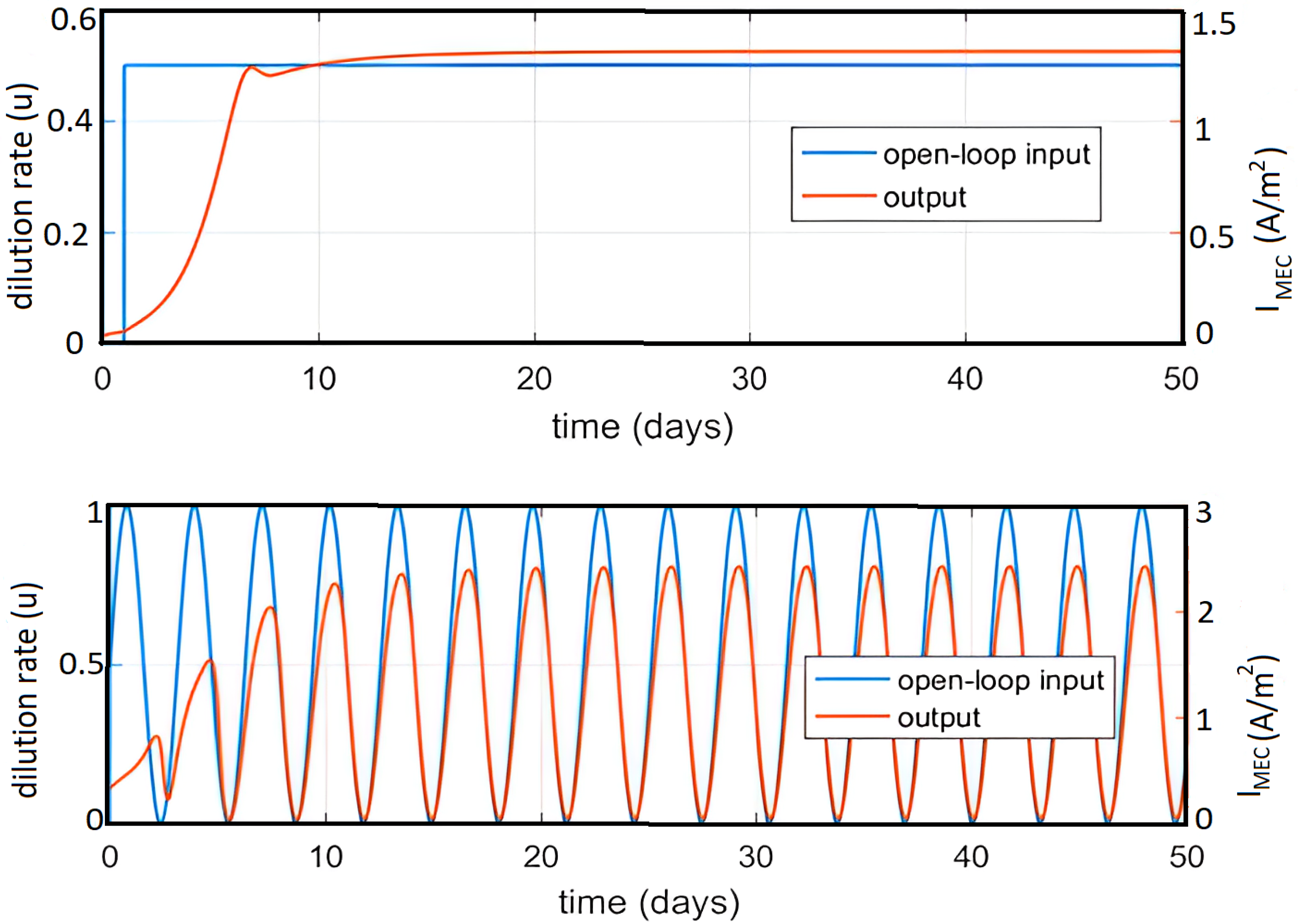
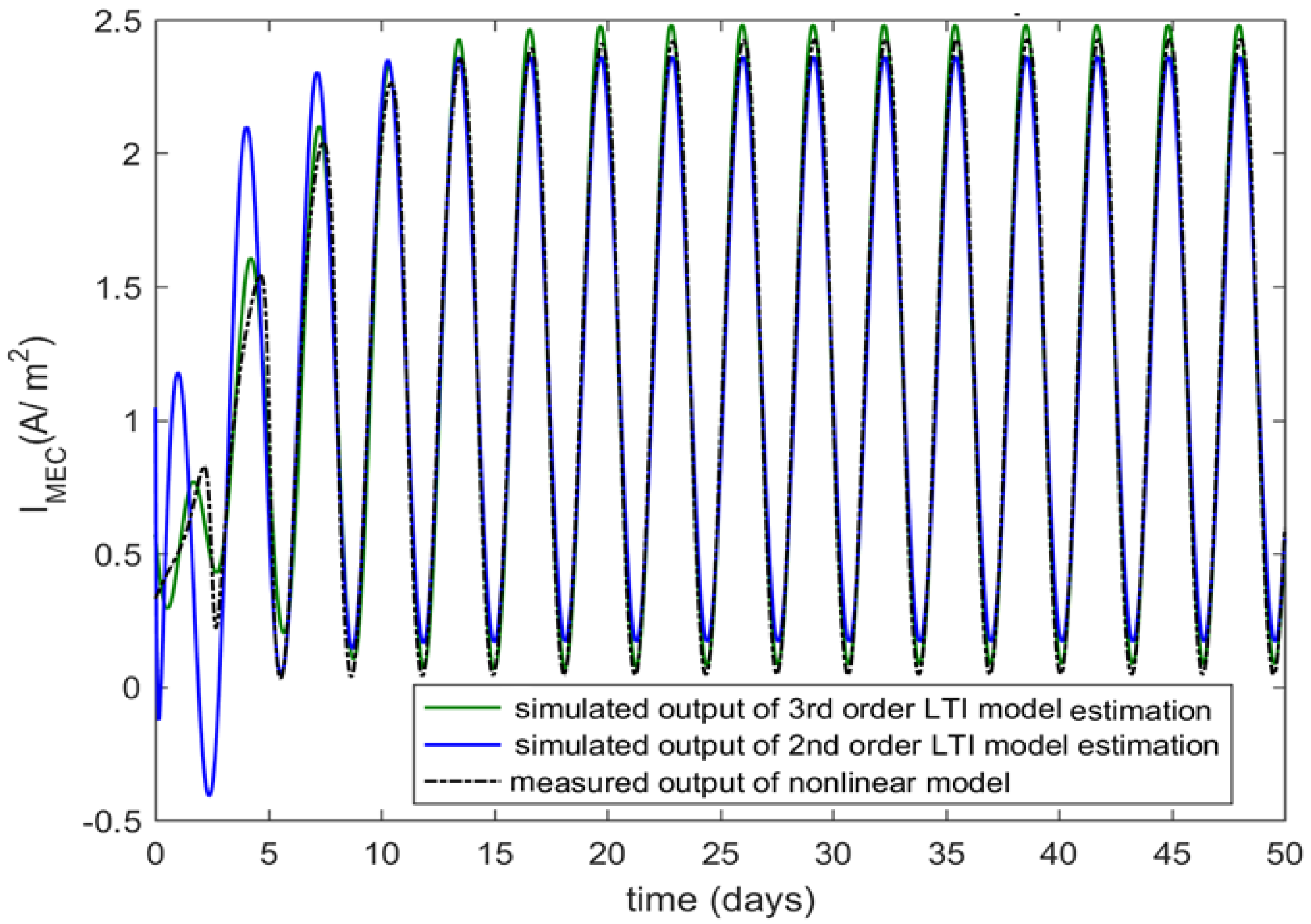
2.3. LTI Model Estimation for a Continuous MEC Reactor Process

The suggested fixed-structure H controller is a linear and designed using non-smooth H optimization. The LTI process model is required to optimize the parameters of this robust H controller while keeping its desired structure. To create the conventional H synthesis, GA-PID, and traditional PID, the LTI model must also be determined.
Figure 4 shows the input and output sinusoidal waveform data, which were gathered for linear model estimation. Note that the sinusoidal input–output data are helpful for system identification. Thus, based on the sinusoidal data gathered, an acceptable LTI model was discovered using the MATLAB system identification toolbox. This toolbox works in four steps. The system’s input–output data collection and the model’s structural determination are necessary for the first and second steps, respectively. The defined structure’s parameter estimate is obtained in the third stage, and the model validation and accuracy calculation are done in the final step. The accuracy of this estimation is calculated by comparing it with the nonlinear model’s data. The MATLAB identification toolbox calculates the mean square error to define this accuracy. In Figure 5, the nonlinear and estimated LTI models are compared. Two structures were estimated: (i) second-order model; and (ii) third-order linear model. Based on the expression given by
G 1 ( s ) = 32.07 s + 18 s 2 + 15.1 s + 7.109 ,
we provide an approximation of the second transfer function with a 74.9% accuracy. From the formulation stated as
G 2 ( s ) = 1.672 s 2 + 1.664 s + 2.717 s 3 + 0.7187 s 2 + 4.584 s + 1.058 ,
we obtained an approximation of the third-order transfer function with an accuracy of only 94.08%. The third-order LTI model was considered for the design of conventional and advanced robust control schemes.
Figure 5 shows that the chosen model closely matches plant behavior. The linear traditional PID, conventional H , GA-PID, and fixed-structure H controllers are designed in the following section using the LTI model.

3. Design of Controllers for a Continuous MEC System

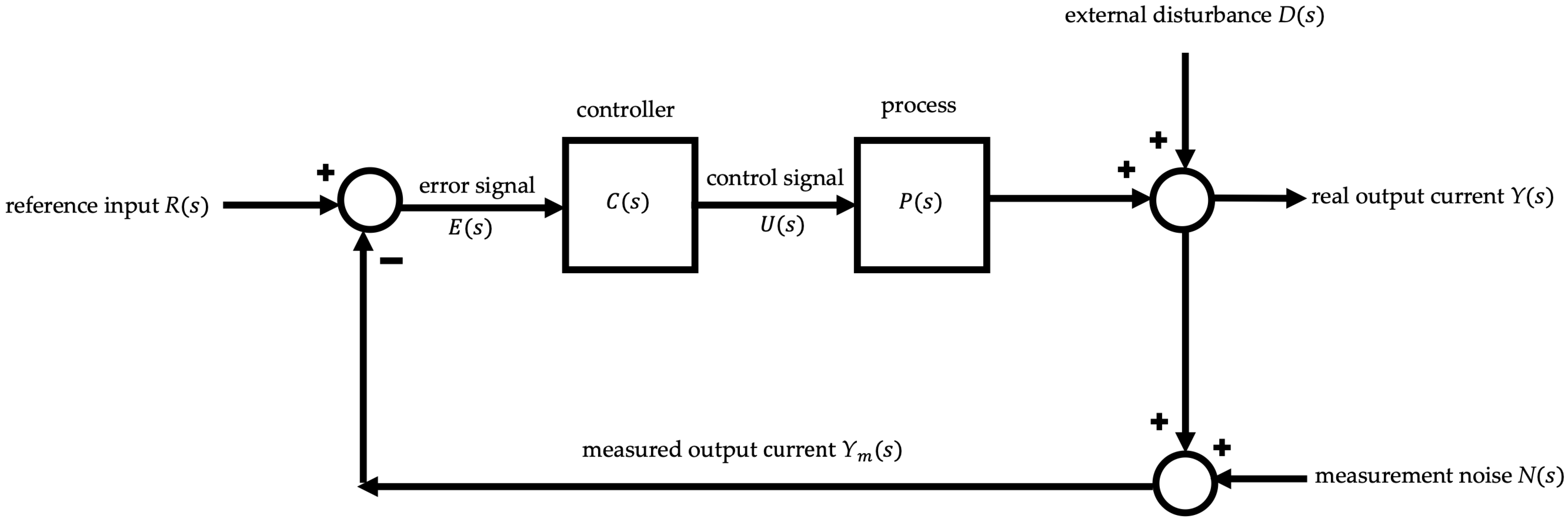
3.1. Statement of the Problem

The problem is solved creating an appropriate controller to precisely track the commanded input. Based on the LTI model, estimated in Section 2, four controllers were designed, and the outputs were analyzed. They are traditional PID, conventional H synthesis, GA-PID, and fixed-structure H controllers, and the output current is the variable that needs to be controlled. The cornerstone for defining the performance standards for all control techniques is tracking the commanded signal. However, the performance metrics used to evaluate the system output include overshoot, settling time, and steady-state error.

3.2. Conventional Design of a PID Controller

PID controllers are widely utilized worldwide because they are low cost and easy to use. The conventional design of PID controllers is less effective if the nonlinearity is included in the dynamic model, since it does not offer flawless tracking and exact performance parameters. PID controllers have been developed over the years using traditional tuning methods, including the Ziegler–Nichols, pole-zero placement, root locus, and Skogested-IMC methods [43]. In the MATLAB single-input single-output (SISO) toolbox, a traditional PID controller utilizing the Skogestad-IMC root locus technique was designed.
An LTI transfer function of continuous MEC process was employed for a conventional PID design. From the expressions given by
U ( s ) = K p + K i 1 s + K d s E ( s ) u ( t ) = K p e ( t ) + K i 0 t e ( τ ) d τ + K d d d t e ( t ) ,
we obtain the transfer function and time domain equations, respectively, of the traditional PID controller, where the tuning parameters of the conventional PID are differential gain ( K d ), proportional gain ( K p ), and integral gain ( K i ), where U ( s ) is the signal control at domain s and u ( t ) is the signal control at time t; E ( s ) is the signal error at domain s and e ( t ) is the signal error at time t. The results of this conventional design are presented and discussed in Section 4.

3.3. Design of a Conventional H Synthesis

The conventional H controller is constructed using smooth H optimization in the frequency domain [44]. The magnitudes of the closed-loop sensitivity transfer function, that is, S ( s ) , and the complementary sensitivity transfer function, that is, T ( s ) , are sculpted by complex weights. Note that T ( s ) is the closed-loop transfer function between reference input R ( s ) and output Y ( s ) , whereas S ( s ) is the closed-loop transfer function between reference R ( s ) and E ( s ) . Note that S ( s ) = 1 / ( 1 + G C ) and T ( s ) = G C / ( 1 + G C ) , where L = G C is the loop transfer function. For a typical H controller, the H norm, which symbolizes the peak value of weighted frequency domain sensitivity S ( s ) or its complementary sensitivity T ( s ) , is reduced. Observe that w S S ( s ) 1 and w T T ( s ) 1 contain the constraints (peak specs) for modifying the controller parameters, where w S and w T are shaping weights of the closed-loop and complementary sensitivity transfer functions.
Since sensitivity represents the effectiveness of the closed-loop, it should ideally be very low. The peak requirements show a margin of robustness and avoid high-frequency noise amplification. The H controller performs better than a traditional PID controller. The shaping weights and constraints are defined using the MIXSYN MATLAB tool. Based on the defined weights and constraints, the robust MIXSYN tool of MATLAB optimized a state-space structure of the H controller to obtain robust performance. However, the order of this H controller is equal to the order of the process model plus the order of the weights used to shape closed loops S ( s ) and T ( s ) , which is a significant shortcoming of the H controller. This might not be a big deal in typical applications with plenty of computational resources, but in an industrial process setting, it is often a problem. The state-space results for the design of the H controller are presented in Section 4.

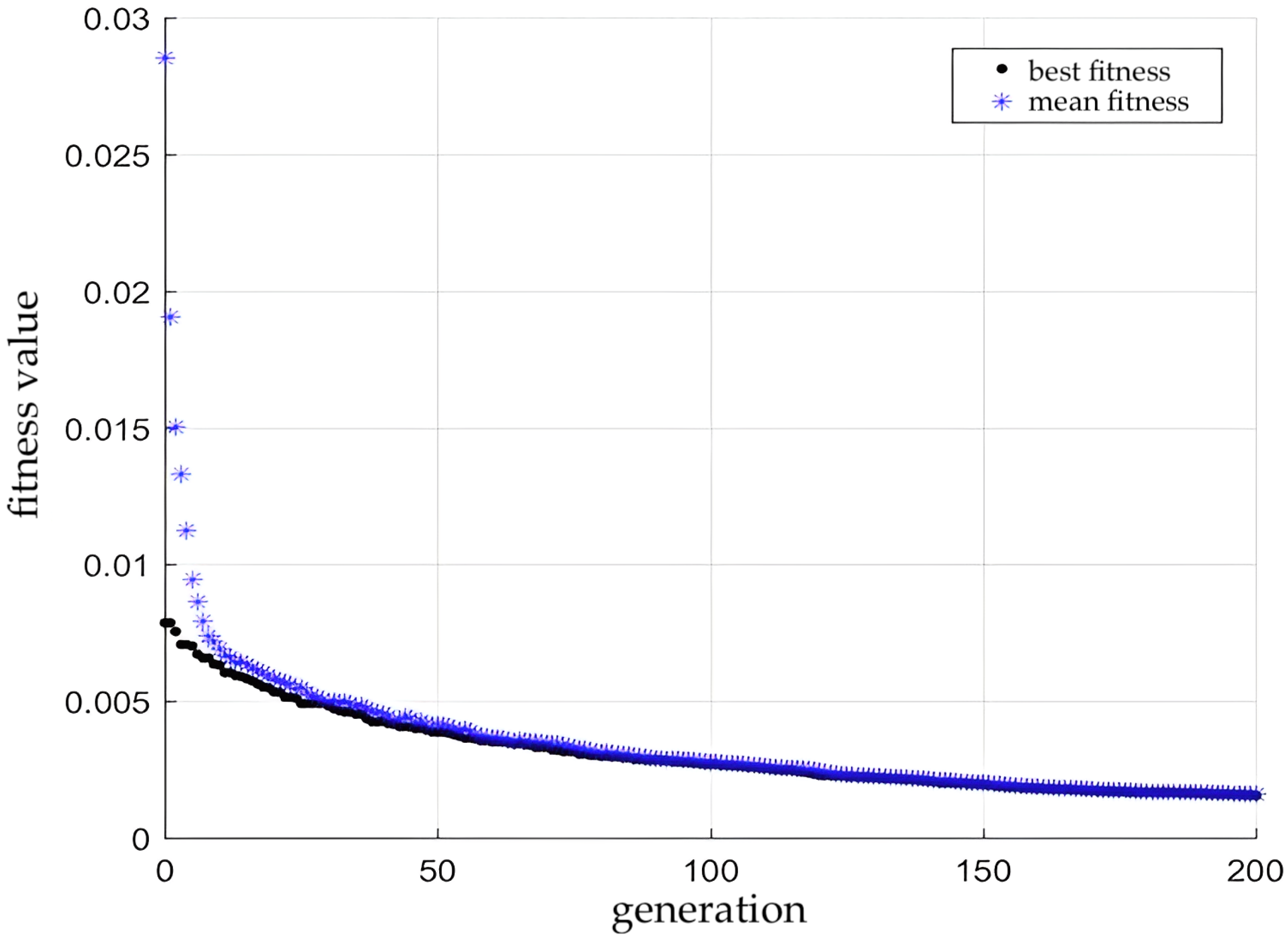
3.4. Design of the Genetic Algorithm for a PID Controller

The GA is a stochastic search technique that can be utilized to optimize challenging situations, including the case of both linear and nonlinear systems of equations. Instead of employing deterministic principles, the GA uses random transition rules and manages a population of alternative solutions termed individuals. Through an iterative process, a new generation of individuals is built by altering the chromosomes of the individuals of the current generation, as we can see in [45]. The fitness of every individual is evaluated using the objective function. The GA performs mainly three operations: mutation, crossover, and selection. Suppose that a GA is used to minimize an objective function f. Then, individual sol a is said to be a better solution than individual sol b if and only if f ( sol a ) < f ( sol b ) . This is the fundamental criterion in the selection operation of a GA. This optimization has high efficiency, but with a high computational cost as well.
In Algorithm 1, we can see the basic steps of a GA [46]. We used this simple approach to carry out our computational experiments. Regarding the GA input, f is the function to optimize, n is the number of individuals in each generation (population size), and iter defines the number of iterations—that is, the number of generations to be built. Just before ending, the GA returns the best solution found bestSol, and the value obtained bestFit, by evaluating the best solution in the objective function f. The best fitness results for a GA-PID design for the continuous MEC process are given in Section 4.
Algorithm1: General structure of a GA
Fractalfract 06 00736 i001

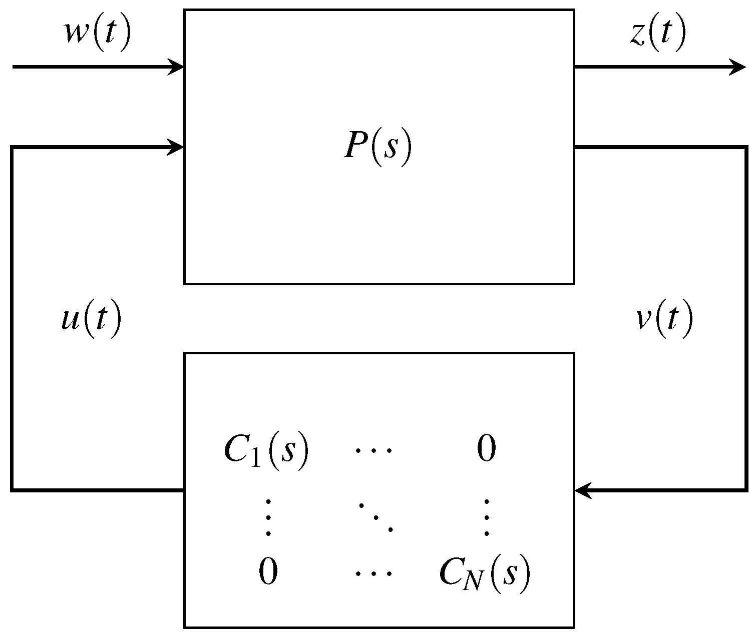
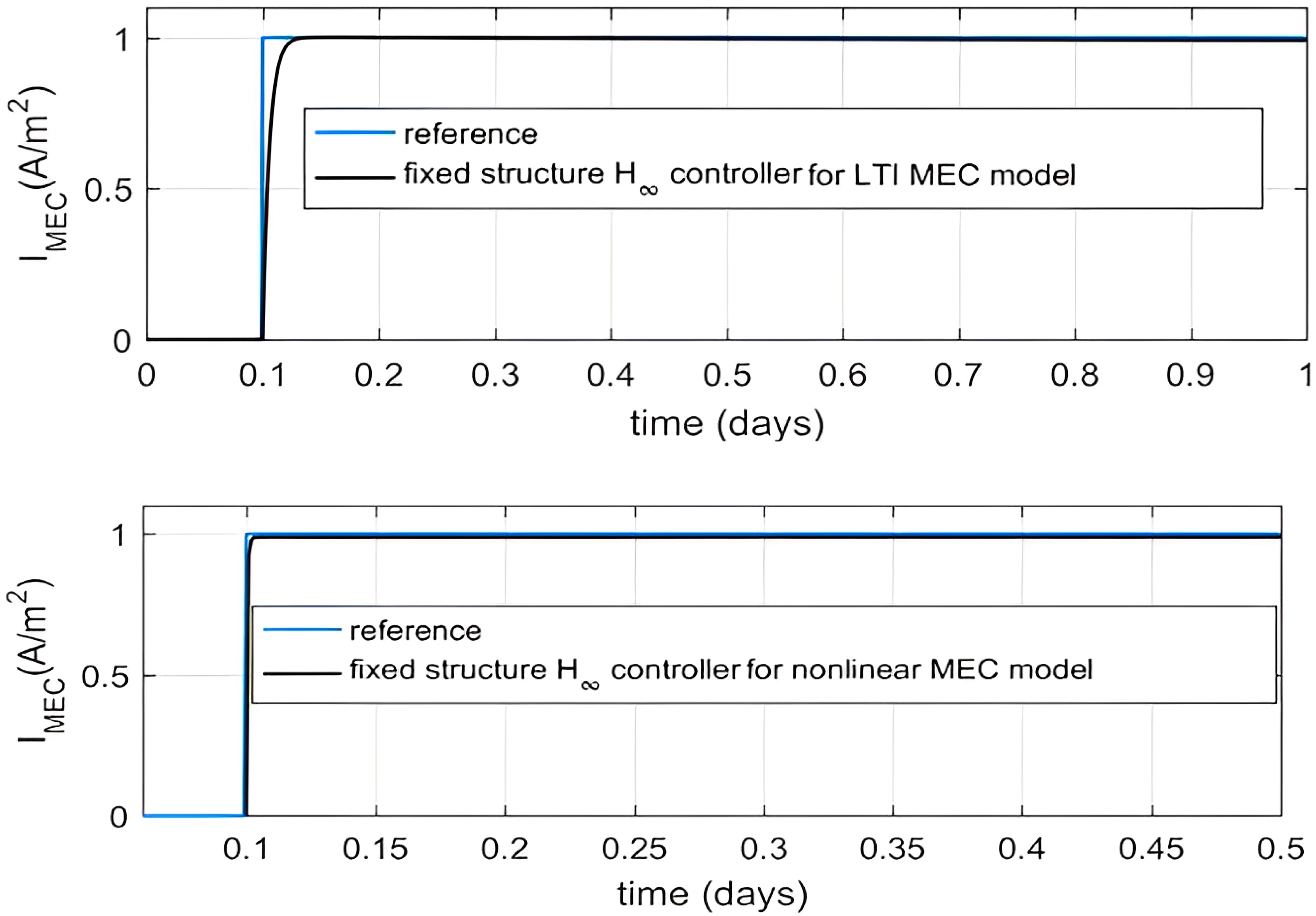
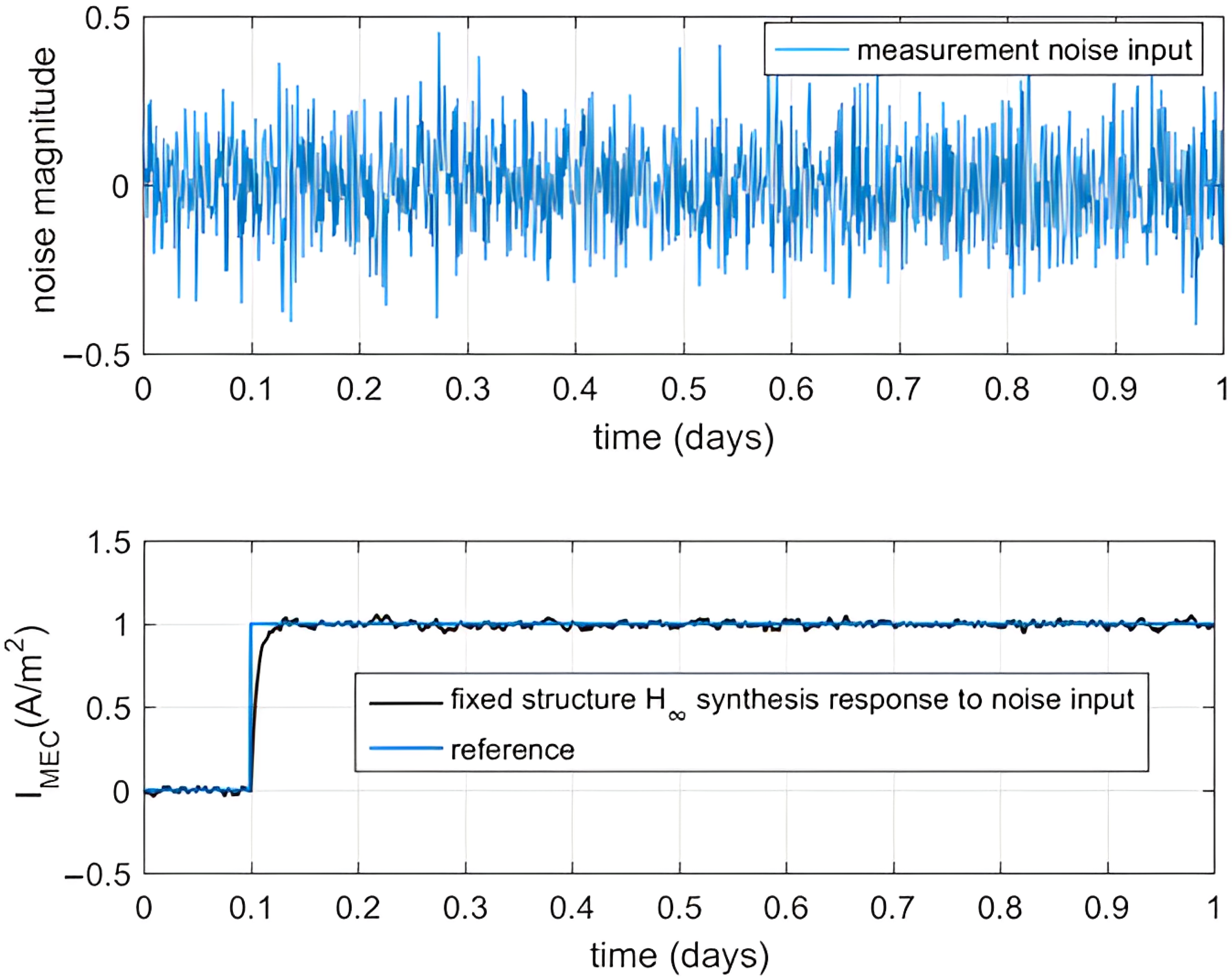
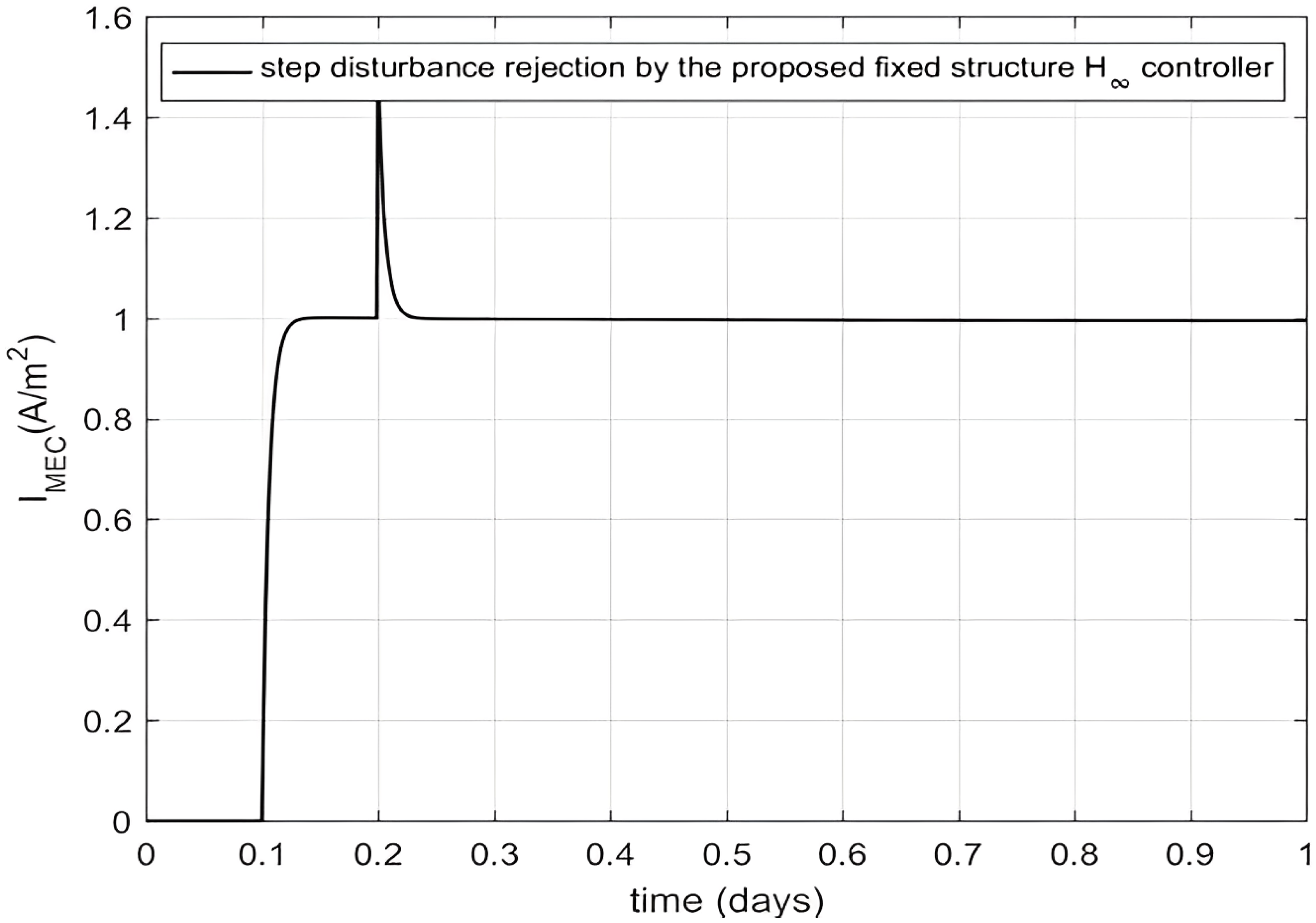
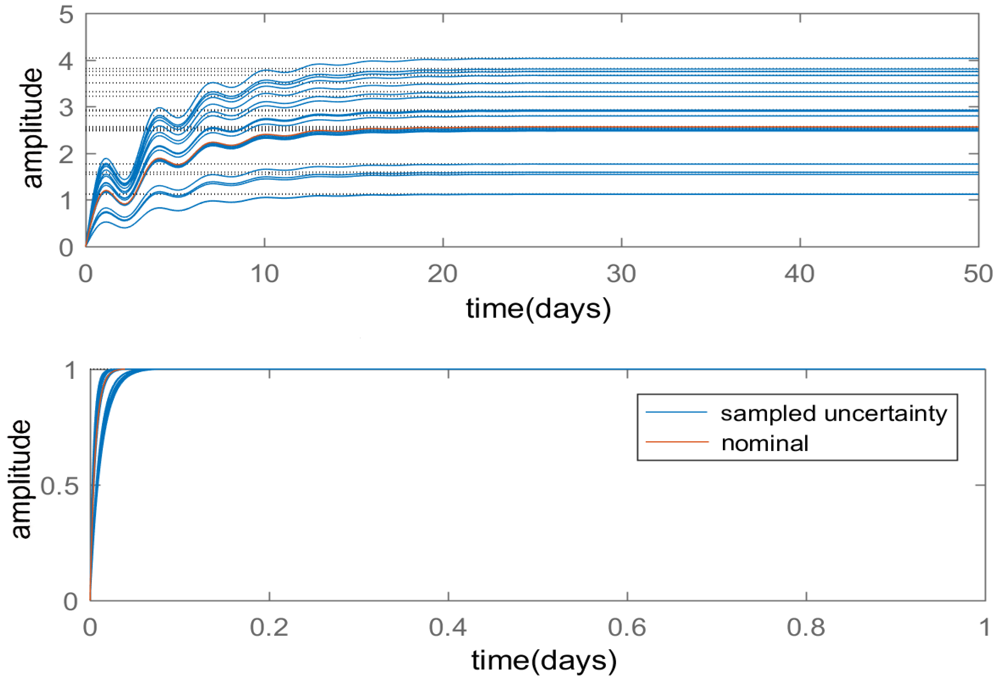
3.5. Design of the Proposed Fixed Order and Structured H Synthesis

Due to monolithic design and practical restrictions, conventional H controllers have seen slow industry adoption. The norms of conventional H controllers are further constrained by complex structure and design specifications, including response time and control bandwidth [47]. High-order complex weighting filters may be utilized to improve the results. By employing non-smooth H optimization in the frequency domain, the suggested robust optimization adjusts the essential control elements, such as PIDs. However, this complicates the structure of the ordinary H controller. The constraints of the conventional H controller are all overcome by fixed-structure H controllers. The fixed-structure-based controllers have more practical importance and execute well in terms of response time and quality of the solution [47]. The fixed and non-tunable elements, tunable control block, and standard formulation of the proposed fixed-structure H synthesis are all represented in the following paragraph.
Figure 6 displays the standard form of H synthesis, which consists of two key components: (i) the block P ( s ) , which contains all the non-tunable (fixed) components of the whole control system, such as an LTI model of the continuous MEC process; and (ii) the second block, which contains the proposed synthesis required structure and fixed-order control elements. In the case of sophisticated multi input multi output (MIMO) systems [31], all these elements are tunable. When it comes to SISO systems, this block contains just one configurable control element. The customizable diagonal block of tunable control components allows for decoupling complex MIMO processes, where each control element C i ( s ) has a known structure, which is presumed to be an LTI, and is established from
C ( s ) = C 1 ( s ) 0 0 C N ( s ) .
In Figure 6, the tunable elements are placed in block/controller C ( s ) , and the remaining elements are placed in block/process P ( s ) . The error signal e ( t ) is aggregated in z ( t ) = y ( r ) r ( t ) , with y ( t ) being the current measurement and r ( t ) is the reference input, whereas the external input, including the external disturbance D ( s ) , measurement noise N ( s ) , and reference inputs, are merged into w ( t ) . The partition of the standard representation is given by
z ( t ) v ( t ) = P w ( t ) u ( t ) = P 11 P 12 P 21 P 22 w ( t ) u ( t ) ,
where u ( t ) is the signal control. The closed loop objective function formulation from w ( t ) to z ( t ) is represented in linear fraction transformation form [47] as
T w ( t ) z ( t ) ( s ) = F l ( P , C ) = P 11 + P 12 C ( I P 22 ) 1 P 21 .
Optimizing the parameters of the tunable control elements, such as tunable PIDs, is another difficult task. Scalars such as K p , K i , K d , and T f are used as parameters for the transfer function of the PID controller, which is found by taking the Laplace transform with its variable s, and obtained as
C j ( s ) = K p + K i s + K d s T f s + 1 .
Parameters K p , K i , K d , and T f are tuned by non-smooth H optimization. For the controller structure to be effective and practical, the derivative control term is made up properly using coefficient T f as the time constant of the first-order filter.
Next, we detail how to optimize the suggested fixed-structure H synthesis. The controller settings are adjusted in the frequency domain to adhere to standard design criteria. In the case of a SISO system, we must minimize the H norm, which consists solely of the maximum values of the closed-loop transfer functions S ( s ) and T ( s ) across the entire frequency range. The standard form of the objective function H ( s ) is provided as
H ( s ) = F l ( P ( s ) , diag ( C 1 ( s ) , , C N ( s ) ) ,
whereas from the constraints stated in (8), we can formulate the criteria for resilient design, such as external and internal disturbance rejection, noise elimination, high stability margins, improved control bandwidth, and enhanced transient specifications.
The appropriate complex weighting transfer functions w S and w T were selected to provide the desired forms of the closed-loop transfer functions S ( s ) and T ( s ) , respectively. The intended forms of S ( s ) and T ( s ) follow the design specifications stated as W j ( s ) T j ( s ) 1 , for j { 1 , , M } , and W i ( s ) S i ( s ) 1 , for i { 1 , , N } . The proposed fixed-structure H synthesis is independent of the complex weight order.
The structure of conventional H synthesis is bound by the order of the complex shaping weights. In the case of a conventional H controller, a more complex structure arises by using a high order shaping weights to enhance the robustness. For the LTI model of the MEC process in a continuous reactor, C ( s ) is a parametrically optimized and tuned robust PID controller. In MATLAB, the generalized form of the prescribed H synthesis problem is coded as follows:
  • C ( s ) = ltiblock.pid(‘C’,‘pid’);
  • S ( s ) = feedback(1,G(s)*C(s));
  • T ( s ) = feedback(G(s)*C(s),1);
  • H 0 = blkdiag(W s *S(s),W T *T(s));
where S ( s ) = tf(1/M wb, 1 wb*A) and T ( s ) = 0.001 .
The generalized state-space structure ( H ( 0 ) formulation) has two outputs, two inputs, nine states, and a block C ( s ) , which is a robust PID controller to be tuned. The structured controller must optimize all its parameters by a fast and robust algorithm [41]. The suggested optimization starts with randomly chosen values of the structured controller parameter and concludes with required resilient parameter values that adhere to the predetermined limitations. To obtain the resilient optimal control parameters through the non-smooth H optimization, the generalized H ( 0 ) formulation is transformed into the H ( s ) form—that is, the standard form of the objective function stated in (8). The HINFSTRUCT tool in MATLAB helped this optimization. The HINFSTRUCT tool employs the fast optimization and robust algorithm [41] and adjusts the parameters by minimizing the closed-loop objective function gain between the system’s inputs and outputs. Figure 7 depicts the schematic diagram for the system’s basic feedback loop design, and Section 4 compares the simulation results of the structured H synthesis with those of traditional and intelligent controllers.

4. Comparison, Discussion, and Conclusions

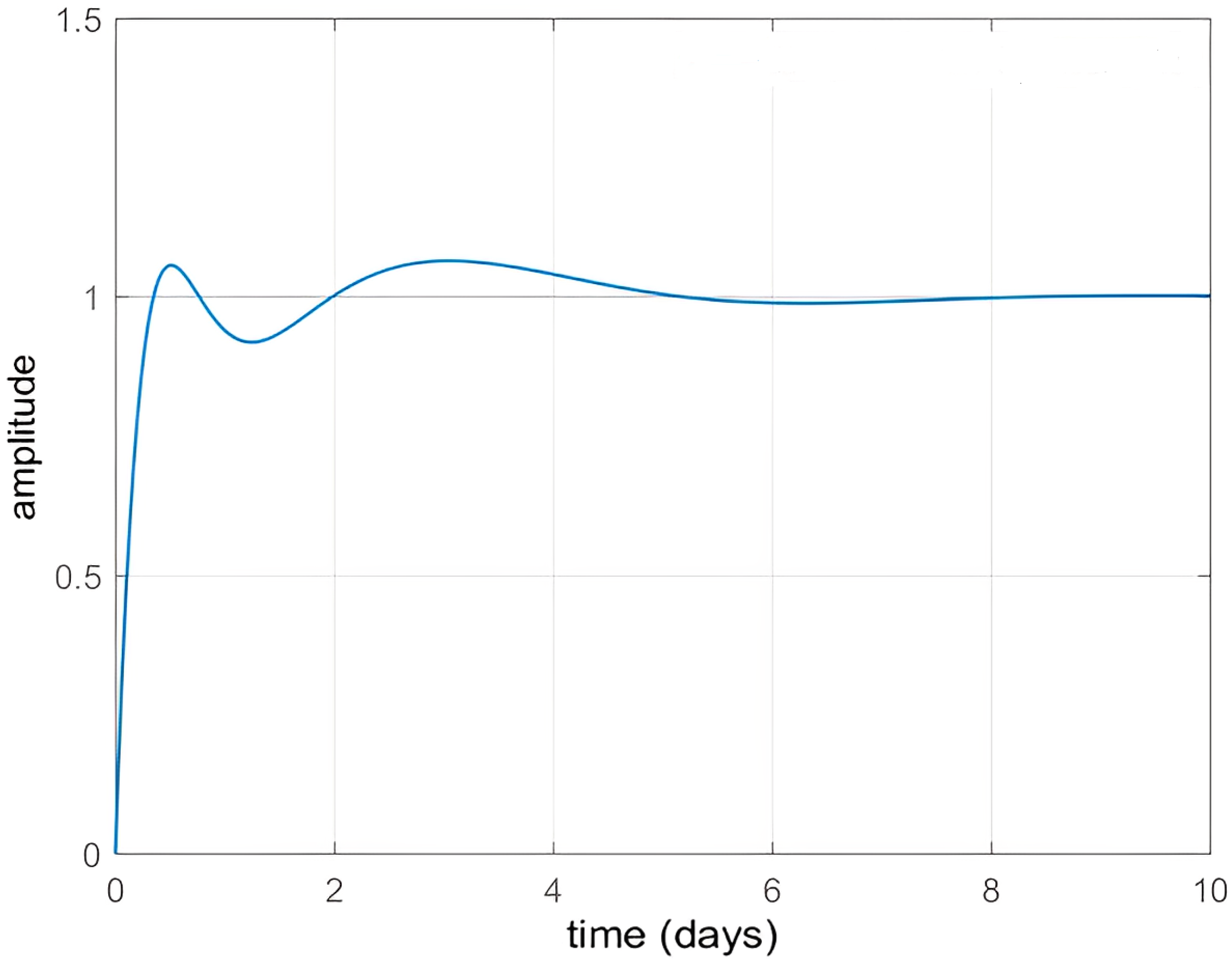
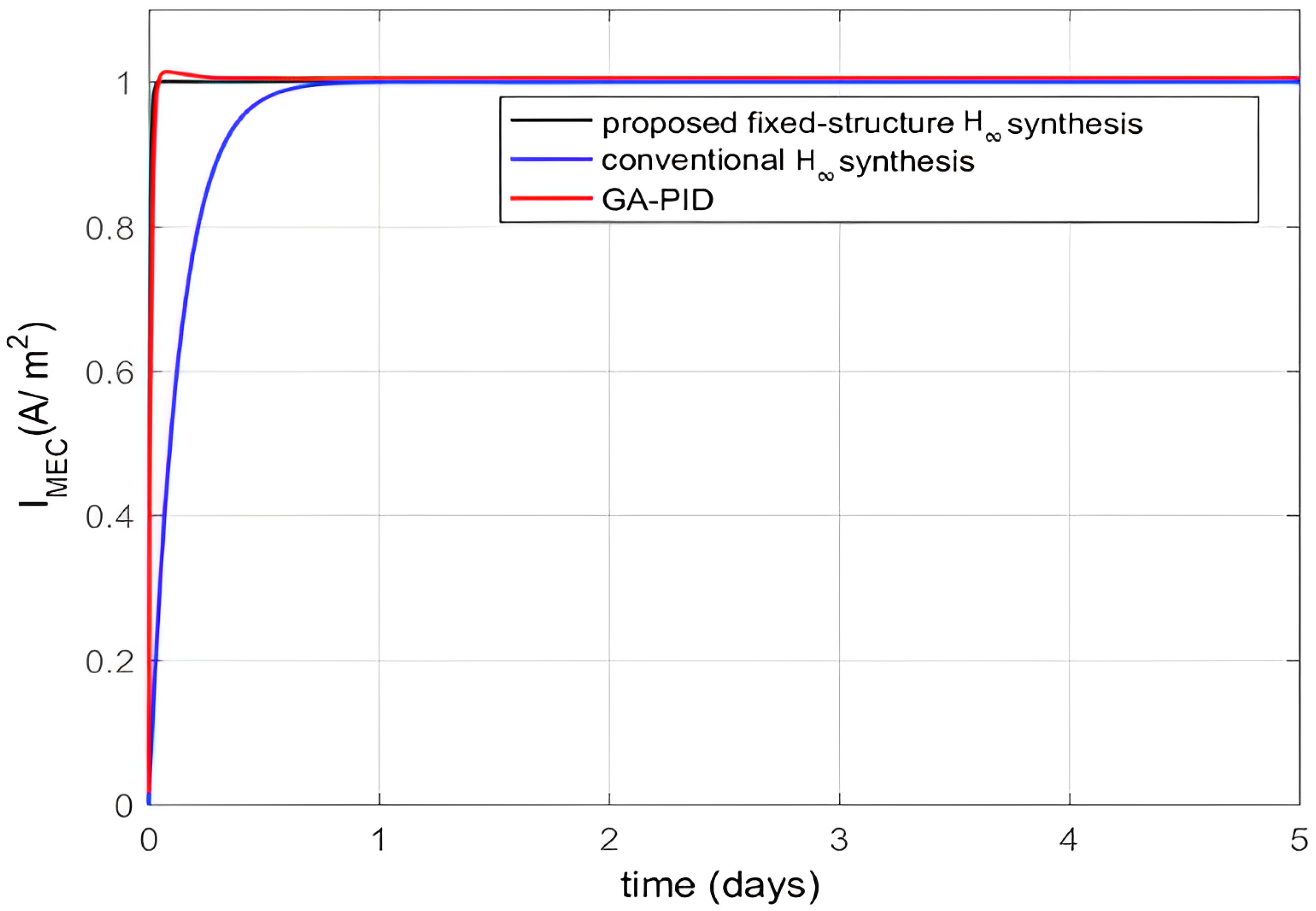
4.1. Performance Comparison and Discussion

The process dynamics are defined by the state-space representations used to build intelligent and robust linear controllers. An LTI model is first computed for the continuous MEC reactor process. Due to their low cost and ease of use, PIDs are widely utilized in industrial processes. Nevertheless, due to the nonlinear dynamics of the process, traditional PIDs cannot accurately regulate the dynamic behavior of their parameters. The calculated parameters (gains) for the Skogestad-IMC PID controller are K p = 3.5086 , K i = 5.8477 , and K d = 0.001 .
Figure 8 displays the step response for the conventional PID controller, whose response exhibits the overshoot and takes roughly five days to settle, which is not a good performance.
The conventional H controllers get beyond the drawback of traditional PIDs, but they also have architectural restrictions. These high-order robust controllers have practical limitations because of the complexity of their structure. It is essential to highlight that this investigation considers the same complex shaping weights for the proposed fixed-structure and conventional H controllers. Thus, we provide an accurate comparison between these two robust controllers regarding their structures and transient and steady-state performances. The calculated state-space structure of the conventional H synthesis, which is a fourth-order controller, is given by
A = 5 × 10 10 0 1.11 × 10 16 2.22 × 10 16 3.114 × 10 4 6950 3459 5646 0 2 0 0 0 0 1 0 B = 0.08703 0 0 0 C = 3.577 × 10 5 7.984 × 10 4 3.971 × 10 4 6.486 × 10 4 D = 0 .
The cost of the controller increases due to its high-level structure. The GA-PID was created for the continuous MEC reactor process as a helpful structural controller, utilizing an intelligent optimization technique. The efficiency of this optimization grows with the population size, albeit at a high computational cost. Figure 9 depicts the convergence of the GA-PID with 200 generations. The optimized parameters for GA-PID are K p = 206 , K i = 5.5 × 10 3 , K d = 32.7 , and T f = 0.5 . As mentioned, we designed a fixed-structure H control synthesis for a continuous MEC system. The accurate tracking of commanded signals, a significant issue in process industries, is one of the ultimate goals of this design. Fixed-structure H syntheses are examples of robust optimization-based controllers. They contain simple, streamlined control parts, making them useful in practice. Precision tracking is also achievable with fixed-structure controllers, which have large control bandwidths to accommodate parameter uncertainty, measurement noise, and disturbance effects. Table 4 lists the optimum parameters for the proposed fixed-structure H synthesis.
Note that we used a total of four controllers. The first controller was a conventional PID one (the Skogestad-IMC PID), and its results are presented in Figure 8, whereas the other three controllers were optimal or robust, and their results are presented in Figure 10, which illustrates the simulation results for the comparative examination of three optimized controllers for step reference input. The outcomes of the suggested synthesis are also relatively better regarding the transient and steady-state responsiveness, as shown by this figure.
The proposed fixed-structure H synthesis for step input tracking has reduced rise time, overshoot, and settling time, according to evident simulation findings. Figure 10 shows that the proposed fixed-structure H synthesis and the GA-PID both exhibit the same rising time approximately, and then they are more efficient than the traditional H synthesis. In addition, both H syntheses eliminate overshoot, whereas the GA-PID produces a slight overrun. Based on transient step response criteria, Table 5 compares all controllers. In summary, all three optimized controllers outperform the conventional PID.
We linearized the model to create robust controllers. Then, we evaluated the proposed controller’s resilience on both linear and nonlinear models. Additionally, we used a linearized plant model to acquire reliable characteristics due to the optimal synthesis settings, which is improved, reliable, and robust. Furthermore, the robustness of the parameters of these controllers can be assessed on both linear and nonlinear models. Similarly, in our case, fixed-structure H controllers are linear, durable, and optimized. These controllers work well for both linear and nonlinear models of the same process. The proposed controller implementation for linear and nonlinear models of a continuous MEC reactor process is shown in Figure 11, and we can see robustness in both cases. The proposed fixed-structure H controllers have unusual noise and disturbance rejection performance. Figure 12 illustrates how the suggested fixed-structure H controller eliminates noise. Figure 13 depicts the proposed controller’s response to the deployment of a step interruption of 0.5 magnitudes. Step disruption occurred after 0.2 days. The simulation results in Figure 13 show that after rejecting the step disruption, the recommended controller resumed tracking of the reference in less than 0.02 days.
As robust controllers are designed to handle uncertainty, they maintain the correct response, even in the presence of uncertain parameters which would otherwise cause instability or an undesirable response. Both traditional H and robust fixed-structure H controllers performed well with about plus or minus 50% variations in nominal parameters of this continuous-reactor plant model. To show the robustness of the proposed method, a wide range (plus or minus 40%) of parameter variation has been considered, as shown in the first graph of Figure 14. The proposed synthesis maintained the desired performance at low costs to rising time and settling time, as shown in the second graph of Figure 14.

4.2. Conclusions

MEC processes performed in continuous reactors and using organic wastewater dilution rate input are growing renewable technologies for treating this type of water and creating hydrogen. The newly created renewable MEC technology needs feedback control to produce the best required output. Minimal literature on the mathematical modeling and regulation of novel MEC processes is available. A dynamic mathematical model of a continuous MEC system concerning control applications was put forth in [31], but no control design has yet been proposed. We computed the LTI model for the first time by linearizing the state-space model at the nominal operating point. Then, four distinct linear control schemes were designed using the LTI model.
The MATLAB software was utilized for all control strategies in the simulation. The proposed fixed-structure H approach was compared with three developed controllers, including the traditional H , intelligent GA-PID, and conventional PID controllers. Table 5 reported the effectiveness of the proposed robust control strategy concerning transient specifications. Regarding disturbance and measurement noise rejection, our fixed-structure H synthesis performed remarkably well. The proposed controller was created using an LTI model, and its implementation produced very good results for the nonlinear MEC model. The proposed fixed-structure H synthesis is simpler and more decentralized than the traditional H controller, which is a considerable advantage. The efficiency of the proposed non-smooth H optimization-based controller can even be enhanced by designing it with high-order shaping weights. Unlike the conventional H controllers, the order of the proposed approach is independent of the order of the complex weights. In addition, its optimal control parameters correspond to the fixed-structure control elements. Compared to the traditional H controller, the intelligent GA-PID controller delivers more reliable outcomes, but the computational cost is very high.
Note that the proposed robust controllers are more usable because they are made up of straightforward control components such as gains and PIDs. Their practical applications go beyond straightforward and solid control. However, it is also possible to build decentralized controllers of complicated MIMO systems employing the proposed synthesis formulation. To the best of our knowledge, the proposed controller is the first one to be developed and applied for the continuous MEC reactor process. Our method performed better than other controllers that we investigated. In future works, we will consider other alternatives to the genetic algorithm, such as particle swarm optimization.

Author Contributions

Conceptualization, M.Z.U.R., V.L., C.M.-B., R.L., and M.R. formal analysis, M.Z.U.R., V.L., C.M.-B. investigation, M.Z.U.R., V.L., C.M.-B., R.L., and M.R. methodology, M.Z.U.R., V.L., C.M.-B., R.L., and M.R. writing—original draft, M.Z.U.R., R.L., and M.R. writing—review and editing, V.L. and C.M.-B. All authors have read and agreed to the published version of the manuscript.

Funding

This research was supported partially funded by FONDECYT, grant number 1200525 (V.L.), from the National Agency for Research and Development (ANID) of the Chilean government under the Ministry of Science, Technology, Knowledge, and Innovation.

Institutional Review Board Statement

Not applicable.

Informed Consent Statement

Not applicable.

Data Availability Statement

Not applicable.

Conflicts of Interest

There are no conflict of interest declared by the authors.

References

  1. Perea-Moreno, M.A.; Hernandez-Escobedo, Q.; Perea-Moreno, A.J. Renewable energy in urban areas: Worldwide research trends. Energies 2018, 11, 577. [Google Scholar] [CrossRef] [Green Version]
  2. Karasmanaki, E.; Tsantopoulos, G. Exploring future scientists’ awareness about and attitudes towards renewable energy sources. Energy Policy 2019, 131, 111–119. [Google Scholar] [CrossRef]
  3. Demirbaş, A. Global renewable energy resources. Energy Sources 2006, 28, 779–792. [Google Scholar] [CrossRef]
  4. Badwal, S.P.; Giddey, S.S.; Munnings, C.; Bhatt, A.I.; Hollenkamp, A.F. Emerging electrochemical energy conversion and storage technologies. Front. Chem. 2014, 2, 79. [Google Scholar] [CrossRef] [Green Version]
  5. Li, H.; Jenkins-Smith, H.C.; Silva, C.L.; Berrens, R.P.; Herron, K.G. Public support for reducing US reliance on fossil fuels: Investigating household willingness-to-pay for energy research and development. Ecol. Econ. 2009, 68, 731–742. [Google Scholar] [CrossRef]
  6. Marques, A.C.; Fuinhas, J.A.; Pereira, D.A. Have fossil fuels been substituted by renewables? An empirical assessment for 10 European countries. Energy Policy 2018, 116, 257–265. [Google Scholar] [CrossRef]
  7. Siddiqui, A.S.; Marnay, C.; Wiser, R.H. Real options valuation of US federal renewable energy research, development, demonstration, and deployment. Energy Policy 2007, 35, 265–279. [Google Scholar] [CrossRef] [Green Version]
  8. Staffell, I.; Scamman, D.; Abad, A.V.; Balcombe, P.; Dodds, P.E.; Ekins, P.; Shah, N.; Ward, K.R. The role of hydrogen and fuel cells in the global energy system. Energy Environ. Sci. 2019, 12, 463–491. [Google Scholar] [CrossRef] [Green Version]
  9. Abe, J.O.; Popoola, A.P.I.; Ajenifuja, E.; Popoola, O.M. Hydrogen energy, economy and storage: Review and recommendation. Int. J. Hydrogen Energy 2019, 44, 15072–15086. [Google Scholar] [CrossRef]
  10. Azwar, M.Y.; Hussain, M.A.; Abdul-Wahab, A.K. Development of biohydrogen production by photobiological, fermentation and electrochemical processes: A review. Renew. Sustain. Energy Rev. 2014, 31, 158–173. [Google Scholar] [CrossRef]
  11. Kadier, A.; Al-Shorgani, N.K.; Jadhav, D.A.; Sonawane, J.M.; Mathuriya, A.S.; Kalil, M.S.; Hasan, H.A.; Alabbosh, K.F. Microbial electrolysis cell (MEC): An innovative waste to bioenergy and value-added by-product technology. In Bioelectrosynthesis: Principles and Technologies for Value-Added Products; Wang, A., Liu, W., Zhang, B., Cai, W., Eds.; Wiley: New York, NY, USA, 2020; pp. 95–128. [Google Scholar]
  12. Montpart, N.; Rago, L.; Baeza, J.A.; Guisasola, A. Hydrogen production in single chamber microbial electrolysis cells with different complex substrates. Water Res. 2015, 68, 601–615. [Google Scholar] [CrossRef] [PubMed]
  13. Kiely, P.D.; Cusick, R.; Call, D.F.; Selembo, P.A.; Regan, J.M.; Logan, B.E. Anode microbial communities produced by changing from microbial fuel cell to microbial electrolysis cell operation using two different wastewaters. Bioresour. Technol. 2011, 102, 388–394. [Google Scholar] [CrossRef]
  14. Cario, B.P.; Rossi, R.; Kim, K.Y.; Logan, B.E. Applying the electrode potential slope method as a tool to quantitatively evaluate the performance of individual microbial electrolysis cell components. Bioresour. Technol. 2019, 287, 121418. [Google Scholar] [CrossRef] [PubMed]
  15. Gandu, B.; Rozenfeld, S.; Hirsch, L.O.; Schechter, A.; Cahan, R. Immobilization of bacterial cells on carbon-cloth anode using alginate for hydrogen generation in a microbial electrolysis cell. J. Power Sources 2020, 455, 227986. [Google Scholar] [CrossRef]
  16. Brogan, W.L. Modern Control Theory; Pearson Education: New Delhi, India, 1991. [Google Scholar]
  17. Li, Z.; Zhang, Z.; Liao, Q.; Rong, M. Asymptotic and robust stabilization control for the whole class of fractional-order gene regulation networks with time delays. Fractal Fract. 2022, 6, 406. [Google Scholar] [CrossRef]
  18. Xu, K.; Cheng, T.; Lopes, A.M.; Chen, L.; Zhu, X.; Wang, M. Fuzzy fractional-order PD vibration control of uncertain building structures. Fractal Fract. 2022, 6, 473. [Google Scholar] [CrossRef]
  19. Skogestad, S.; Postlethwaite, I. Multivariable Feedback Control: Analysis and Design; Wiley: New York, NY, USA, 1996. [Google Scholar]
  20. Picioreanu, C.; Head, I.M.; Katuri, K.P.; van Loosdrecht, M.C.; Scott, K. A computational model for biofilm-based microbial fuel cells. Water Res. 2007, 41, 2921–2940. [Google Scholar] [CrossRef]
  21. Kato Marcus, A.; Torres, C.I.; Rittmann, B.E. Conduction-based modeling of the biofilm anode of a microbial fuel cell. Biotechnol. Bioeng. 2007, 98, 1171–1182. [Google Scholar] [CrossRef]
  22. Pinto, R.P.; Srinivasan, B.; Manuel, M.F.; Tartakovsky, B. A two-population bio-electrochemical model of a microbial fuel cell. Bioresour. Technol. 2010, 101, 5256–5265. [Google Scholar] [CrossRef] [Green Version]
  23. Zeng, Y.; Choo, Y.F.; Kim, B.H.; Wu, P. Modelling and simulation of two-chamber microbial fuel cell. J. Power Sources 2010, 195, 79–89. [Google Scholar] [CrossRef]
  24. Deb, D.; Patel, R.; Balas, V.E. A review of control-oriented bioelectrochemical mathematical models of microbial fuel cells. Processes 2020, 8, 583. [Google Scholar] [CrossRef]
  25. Patel, R.; Deb, D. Parametrized control-oriented mathematical model and adaptive backstepping control of a single chamber single population microbial fuel cell. J. Power Sources 2018, 396, 599–605. [Google Scholar] [CrossRef]
  26. Asrul, M.A.M.; Atan, M.F.; Yun, H.A.H.; Lai, J.C.H. Mathematical model of biohydrogen production in microbial electrolysis cell: A review. Int. J. Hydrogen Energy 2021, 46, 37174–37191. [Google Scholar] [CrossRef]
  27. Gadkari, S.; Gu, S.; Sadhukhan, J. Towards automated design of bioelectrochemical systems: A comprehensive review of mathematical models. Chem. Eng. J. 2018, 343, 303–316. [Google Scholar] [CrossRef]
  28. Azwara, Y.; Abdul-Wahabb, A.K.; Hussaina, M.A. Optimal production of biohydrogen gas via Microbial Electrolysis cells (MEC) in a controlled batch reactor system. Chem. Eng. Trans. 2013, 32, 727–732. [Google Scholar]
  29. Yahya, A.M.; Hussain, M.A.; Abdul Wahab, A.K. Modeling, optimization, and control of microbial electrolysis cells in a fed-batch reactor for production of renewable biohydrogen gas. Int. J. Energy Res. 2015, 39, 557–572. [Google Scholar] [CrossRef]
  30. Alcaraz–Gonzalez, V.; Rodriguez–Valenzuela, G.; Gomez–Martinez, J.J.; Dotto, G.L.; Flores–Estrella, R.A. Hydrogen production automatic control in continuous microbial electrolysis cells reactors used in wastewater treatment. J. Environ. Manag. 2021, 281, 111869. [Google Scholar] [CrossRef]
  31. Flores-Estrella, R.A.; Rodríguez-Valenzuela, G.; Ramírez-Leros, J.R.; Alcaraz-González, V.; González-Álvarez, V. A simple microbial electrochemical cell model and dynamic analysis towards control design. Chem. Eng. Commun. 2020, 207, 493–505. [Google Scholar] [CrossRef]
  32. Alshammari, O.; Kchaou, M.; Jerbi, H.; Ben Aoun, S.; Leiva, V. A fuzzy design for a sliding mode observer-based control scheme of Takagi-Sugeno Markov jump systems under imperfect premise matching with bio-economic and industrial applications. Mathematics 2022, 10, 3309. [Google Scholar] [CrossRef]
  33. Doyle, J.; Glover, K.; Khargonekar, P.; Francis, B. State-space solutions to standard H2 and H control problems. In Proceedings of the 1988 American Control Conference, Atlanta, GA, USA, 15–17 June 1988; pp. 1691–1696. [Google Scholar]
  34. Stein, G.; Doyle, J.C. Beyond singular values and loop shapes. J. Guid. Control. Dyn. 1991, 14, 5–16. [Google Scholar] [CrossRef] [Green Version]
  35. McFarlane, D.; Glover, K. A loop-shaping design procedure using H/sub infinity/synthesis. IEEE Trans. Autom. Control. 1992, 37, 759–769. [Google Scholar] [CrossRef]
  36. Khalil, I.S.; Doyle, J.C.; Glover, K. Robust and Optimal Control; Prentice Hall: London, UK, 1996. [Google Scholar]
  37. Korkmaz, M.; Aydoğdu, Ö.; Doğan, H. Design and performance comparison of variable parameter nonlinear PID controller and genetic algorithm based PID controller. In Proceedings of the 2012 International Symposium on Innovations in Intelligent Systems and Applications, Trabzon, Turkey, 2–4 July 2012; pp. 1–5. [Google Scholar]
  38. Gahinet, P.; Apkarian, P. Decentralized and fixed-structure H control in MATLAB. In Proceedings of the 50th IEEE Conference on Decision and Control and European Control Conference, Orlando, FL, USA, 12–15 December 2011; pp. 8205–8210. [Google Scholar]
  39. Mitchell, T.; Overton, M.L. Fixed low-order controller design and H optimization for large-scale dynamical systems. IFAC-PapersOnLine 2015, 48, 25–30. [Google Scholar] [CrossRef]
  40. Ahmad, M.; Ali, A.; Choudhry, M.A. Fixed-structure H controller design for two-rotor aerodynamical system (TRAS). Arab. J. Sci. Eng. 2016, 41, 3619–3630. [Google Scholar] [CrossRef]
  41. Bruinsma, N.A.; Steinbuch, M. A fast algorithm to compute the H-norm of a transfer function matrix. Syst. Control. Lett. 1990, 14, 287–293. [Google Scholar] [CrossRef]
  42. Pinto, R.P.; Tartakovsky, B.; Srinivasan, B. Optimizing energy productivity of microbial electrochemical cells. J. Process. Control. 2012, 22, 1079–1086. [Google Scholar] [CrossRef]
  43. Borase, R.P.; Maghade, D.K.; Sondkar, S.Y.; Pawar, S.N. A review of PID control, tuning methods and applications. Int. J. Dyn. Control. 2021, 9, 818–827. [Google Scholar] [CrossRef]
  44. Başar, T.; Bernhard, P. H-Infinity Optimal Control and Related Minimax Design Problems: A Dynamic Game Approach; Springer: New York, NY, USA, 2008. [Google Scholar]
  45. Jayachitra, A.; Vinodha, R. Genetic algorithm based PID controller tuning approach for continuous stirred tank reactor. Adv. Artif. Intell. 2014, 2014, 791230. [Google Scholar] [CrossRef]
  46. Mirjalili, S. Genetic algorithm. In Evolutionary Algorithms and Neural Networks; Springer: Cham, Switzerland, 2019; pp. 43–55. [Google Scholar]
  47. Gahinet, P.; Apkarian, P. Structured H∞ synthesis in MATLAB. IFAC Proc. 2011, 44, 1435–1440. [Google Scholar] [CrossRef]
Figure 1. Diagram of a continuous MEC process.
Fractalfract 06 00736 g001
Figure 2. Diagram of the SIMULINK nonlinear state-space model of the continuous-reactor MEC process, where “*” means the multiplication symbol, as usual in programming codes.
Fractalfract 06 00736 g002
Figure 3. Plots of the dynamic behavior of state variables and microorganisms’ growth rates.
Fractalfract 06 00736 g003
Figure 4. Plots of open loop step (first panel) and open loop sinusoidal (second panel) responses of the continuous MEC process.
Fractalfract 06 00736 g004
Figure 5. Plot of generated model results that were validated for sinusoidal input.
Fractalfract 06 00736 g005
Figure 6. Diagram of a standard representation for a structured H synthesis.
Fractalfract 06 00736 g006
Figure 7. Diagram of a feedback loop response for the entire continuous MEC control process.
Fractalfract 06 00736 g007
Figure 8. Plot of the step response for a Skogestad-IMC PID control.
Fractalfract 06 00736 g008
Figure 9. Plot of values for the genetic algorithm PID optimization fitness.
Fractalfract 06 00736 g009
Figure 10. Plot of comparison for controllers with transient specifications.
Fractalfract 06 00736 g010
Figure 11. Plots of the proposed controller implementation for linear (first panel) and nonlinear (second panel) MEC process models.
Fractalfract 06 00736 g011
Figure 12. Plots of randomly generated external noise (first panel) and step tracking of the fixed structure H controller in presence of external noise (second panel).
Fractalfract 06 00736 g012
Figure 13. Plot of the proposed controller’s response to step-disturbance input.
Fractalfract 06 00736 g013
Figure 14. Plots of the plant’s open loop response for parameters uncertainty (first panel) and step input tracking of the fixed structure H controller in presence of parameters uncertainty.
Fractalfract 06 00736 g014
Table 1. Model’s assumptions.
AssumptionsDescription
1Anodophilic microorganisms make up the uniform distribution of the biofilm and are largely adhered to the anode electrode.
2Despite being equally distributed throughout the bulk solution, very little of the acetoclastic methanogenic species are in contact with the anode. Additionally, there can be an excessive number of unattached anodophilic bacteria.
3Multiplying monod kinetics is used to describe the growth of anodophilic bacteria, whereas simple monod kinetics is employed to model the growth of acetoclastic methanogenic bacteria.
4The cathodic chamber is devoid of biomass.
5Acetoclastic methanogenic and anodophili bacteria groups compete with each another for a shared substrate.
6Anodic chamber has the ideal mixture.
7Gradient of concentration of substrate in the biofilm is disregarded.
8Bacteria always have the same amount of the internal electron transfer mediator [42].
9Gas transmission across the membrane is disregarded.
10pH, temperature, and pressure remain unchanged.
Table 2. Mathematical model variables.
VariableDescription
u ( t ) Dilution rate: D ( t )
x 1 ( t ) Substrate bacteria concentration: S ( t )
x 2 ( t ) Anodophilic bacteria concentration: X a ( t )
x 3 ( t ) Acetoclastic methanogenic bacteria concentration: X m ( t )
y ( t ) MEC current density: I mec ( t )
Table 3. Process parameters and their nominal values.
SymbolDescriptionValue
A a Anode area1 m 2
f S 0 Dimensionless fraction0.3
bEndogenous decay rate0.05 d 1
FFaraday constant1.1167 Ad/mole
k a Yield factor for anodophilic0.667 mgS/mgX
k m Yield factor for acetoclastic methanogenic0.667 mgS/mgX
k d , a Decay rate0.04 d 1
k d , m Decay rate0.006 d 1
K S , a Half-rate constant20 M S L 1
K S , m Half-rate constant80 M S L 1
L f Biofilm thickness 25 × 10 6 m
mElectrons per mole2 mole /mol M
PPressure1 atm
RIdeal gas constant8.314 J/mol K
S in Inlet concentration400 mg/L
TTemperature298.15 K
V reac Reactor volume1 L
x 2 ( 0 ) Initial concentration1000 M X L 1
x 3 ( 0 ) Initial concentration100 M X L 1
x 1 ( 0 ) Initial concentration100 M S L 1
Y H 2 Cathode efficiency0.8
Y CH 4 Methane yieldmL CH4/mg S
α a , α m Dimensionless biofilm retention coefficients0.5
γ X Number of coulombs from biomass0.0033 mF/MW X
γ S Number of coulombs from substrate37.22 mF/MW S
η Voltage0.5 V
μ max , m Maximal growth rate0.3 d 1
μ max , a Maximal growth rate1.97 d 1
Table 4. Parameter optimization results of fixed-structure H synthesis.
SymbolsDescriptionValue
K p Proportional gain104
K i Integral gain2.93
K d Derivative gain22.5
T f First order filter coefficient 2.81 × 10 6
Table 5. Comparison of performance for the parameters.
ControlRise TimeSettling TimeOvershootControllerSteady-State
Technique(Days)(Days)(%)OrderError
Traditional PID0.40004.45007.25002nd0.01%
GA-PID0.02100.03391.39942nd0%
Traditional H synthesis0.29290.521804th0%
Fixed-structure H controller0.01250.022102nd0%
Publisher’s Note: MDPI stays neutral with regard to jurisdictional claims in published maps and institutional affiliations.

