3.1. Effective Range of Prefactor
The prefactor
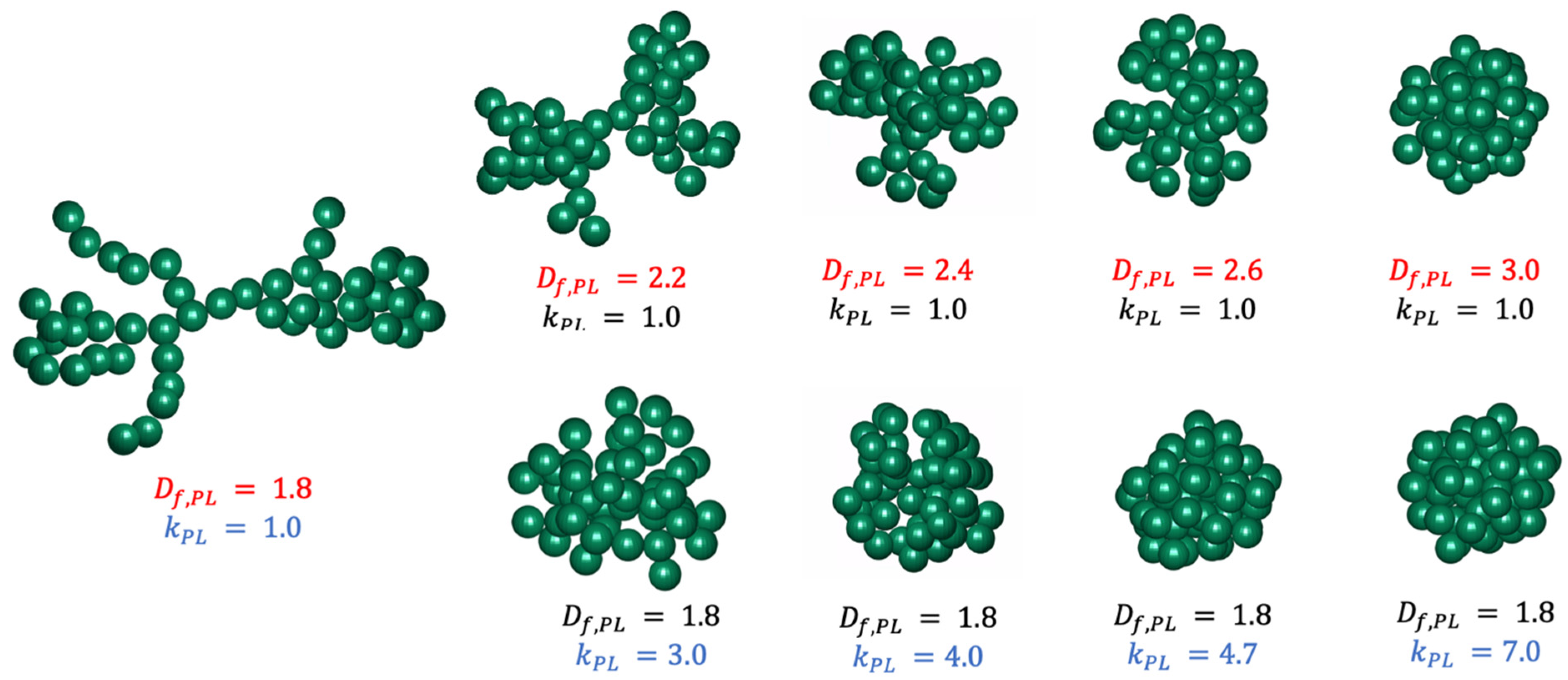
is an important parameter to describe the structural and morphological properties of aggregates, as shown in
Figure 4. Therefore, and with values of
being in the range of 1 to 3, the question arises about the effective range that values of the prefactor
may attain. For a first orientation, we summarized values of
for aggregates with different
from the literature in
Table 1.
Table 1 shows a spread of
from 1.27 to 9.0. However, the variation of
is small in the previous research, and derivations are not always detailed and clear. Therefore, we have decided to test the effective range of
with the help of aggregates generated by the MPTSA model.
In the power law relationship (Equation (1)), the radius of gyration
can describe the spatial mass distribution around the mass center of the aggregate. As a criterion for the effective range of
, we compare the radius of gyration calculated by Equation (1), denoted by
, to the radius of gyration from generated aggregates according to Equation (2), denoted by
. Both
and
are obtained with the same input parameters. The comparison is quantified by the ratio
If of the generated aggregate is greater than 99.99%, then is assumed to have been in its effective range.
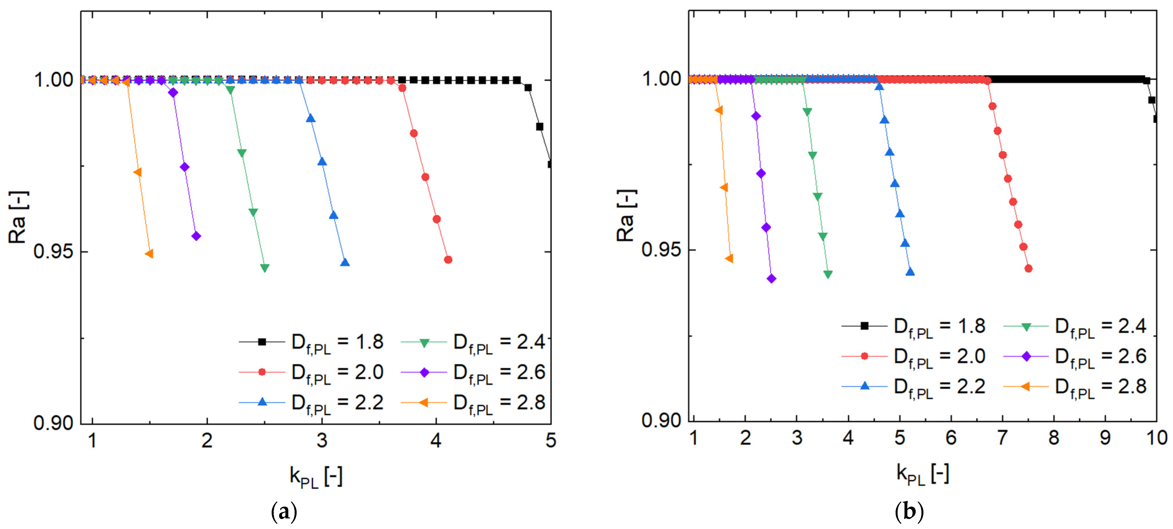
Next, we generated in the frame of this evaluation two groups of aggregates with different fractal dimensions and prefactors. In the first group, the number of primary particles was
= 50, with
= 1.8:0.2:2.8 and
varying from 0.9 to 5.0 in steps of 0.1. As for the second group, it had
= 300,
= 1.8:0.2:2.8, and
= 0.9:0.1:10. The radius of primary particles
was constant and equal to 0.2 mm, but the absolute value of this variable has no influence on the results. The relationship of
and
with
, based on two different values of
, is shown in
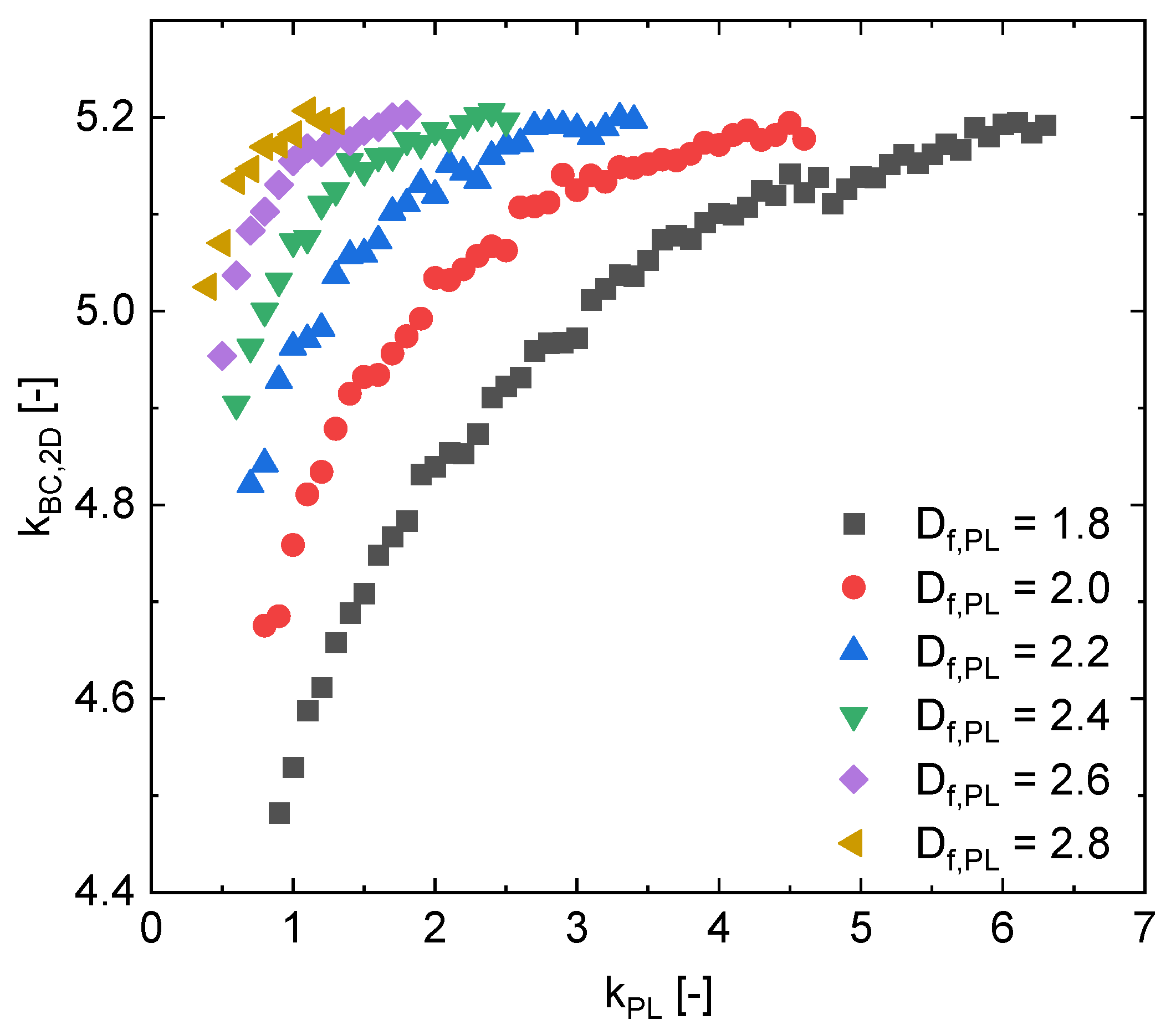
Figure 5.
As can be seen in
Figure 5a,b, all the curves show the same trend: at the beginning,
of the aggregates does not change with increasing
, being on a plateau with
. Then, as
increases, all curves show an inflection point, after which
decreases dramatically. When
is the same, the main difference among the curves is in the length of their plateau regions; aggregates with a smaller
show a longer plateau with
over
. This means that the aggregates with smaller
have a broader effective range of
. Besides, by comparing
Figure 5a,b at the same
, we can find that the effective range of
of aggregates with smaller
(=50) is narrower than in the case of larger
(=300). The horizontal axis coordinates of the inflection points on each curve are considered as the upper limit of the effective range of
under conditions specified by different
and
. Respective values are shown in
Table 2.
In
Figure 5a, when
is larger than 4.7 at
= 50 and
= 1.8, then the
of the aggregates is less than 1. This is since with an additional increase of
(>4.7), the primary particles of these aggregates can no longer be concentrated further in space. So,
of these aggregates does not change with further increasing
. For example, as shown in
Figure 4, the structural and morphological characteristics of the aggregate with
= 1.8 and
= 4.7 are the same as those of the aggregate with
= 1.8 and
= 7.0, with
of these two aggregates being same and equal to 0.74 mm. However,
calculated formally from Equation (1) continues to decrease as
increases, namely from
= 0.74 mm for aggregates with
= 1.8 and
= 4.7, to
= 0.6 mm for aggregates with
= 1.8 and
= 7.0. Therefore, when
= 1.8 and
> 4.7, the ratio
of the aggregates is less than unity, meaning that
has moved outside of its effective range.
As to the lower limit of
, it has been determined by decreasing its value in steps of 0.1. This process stops when the MPTSA model ceases being able to generate the aggregate. Until then, the values of
of the generated aggregates remain equal to 1. The minimum
at which aggregates can be generated is the lower limit of the effective range. Values for different
and
are shown in
Table 2.
In addition to the above method that presupposes the generation of agglomerates by means of the MPTSA algorithm, a much simpler, algebraic estimation of the limits of the effective range of
has also been implemented in the present work. According to Equation (1),
shows a negative relationship to
under fixed
and
,
Therefore, when
and
are fixed and
minimal,
takes its upper limit value. The lower limit of
occurs when the situation is conversed (
at maximum value). The radius of gyration
of an aggregate shows the mass distribution around the aggregate center of mass. In our present work, the radius of primary particles
is constant at 0.2 mm. Therefore, when two aggregates with the same
show different
, the lower value of
indicates that the mass (primary particles) of the aggregate is more concentrated at the center of mass. So, the minimum
is reached when the morphology of the aggregate is like that of a sphere, which is here assumed to happen for an aggregate with
= 3.0 and
= 1.0. On the contrary, the relative gyration radius
of the aggregates is maximum when the primary particles of the aggregates are most dispersed, assumed here to be the case for aggregates with
= 1.7 and
= 1.0. Minimal
(at
= 3.0 and
= 1.0) and maximal
(at
= 1.7 and
= 1.0) of aggregates with different
are calculated by Equation (1), the results are summarized in
Table 3.
Then, minimal
and maximal
of the aggregates with different
are substituted into Equation (10), and upper and lower limits of the effective range are obtained for different
, respectively. The lower and upper limits of the effective range of
that have been estimated in this way are shown in
Table 4.
Comparing
Table 2 and
Table 4, we can find that the upper limit of
obtained by use of the MPTSA model is close (slightly smaller) to the results of the simplified estimation. The lower limit of
in
Table 2 is nearly equal to the lower limit value of
for aggregates with the smallest
(= 5) in
Table 4.
3.2. Relationship between BC Fractal Properties and PL Fractal Properties
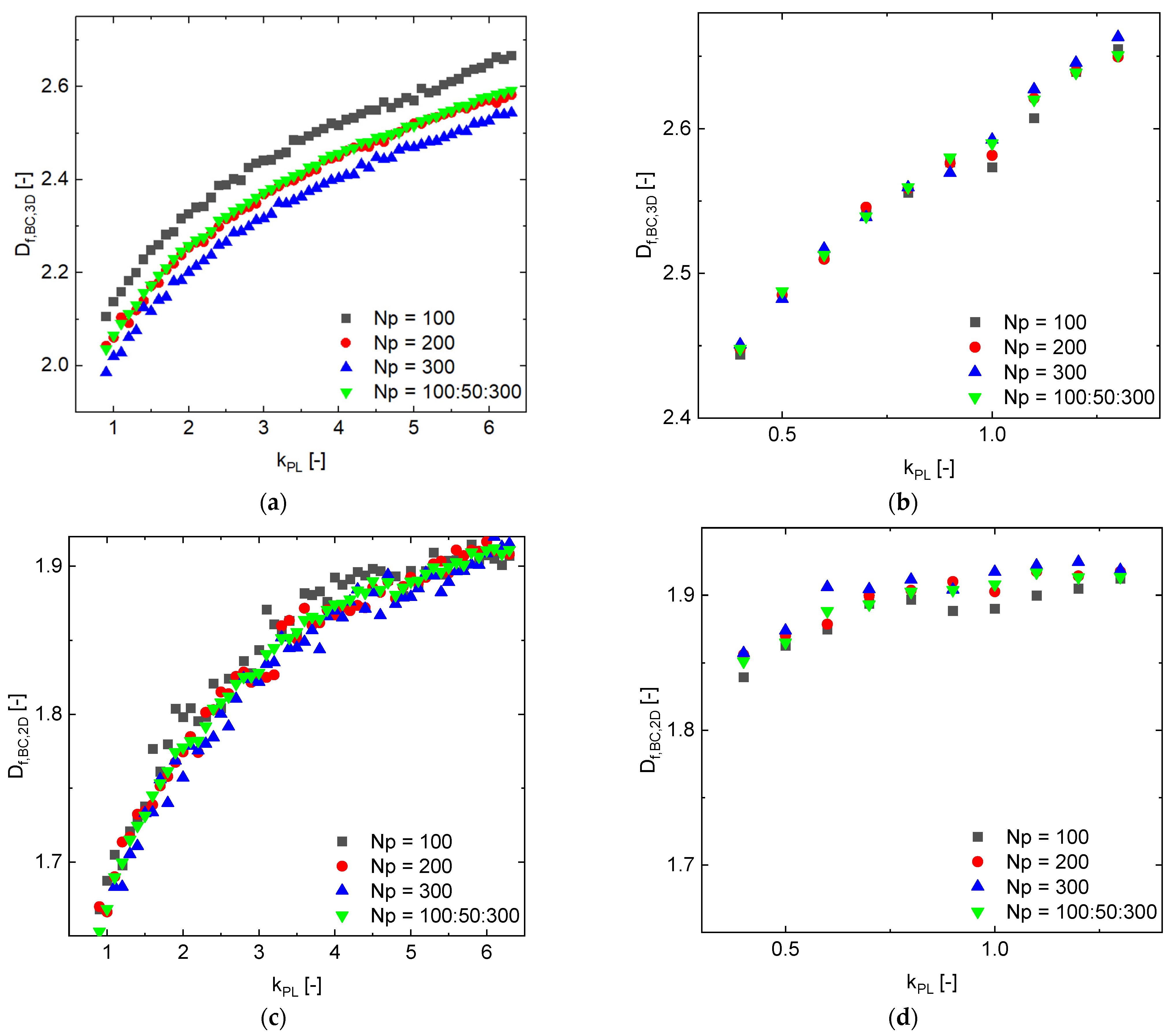
In this section, we generated a series of aggregates with different fractal properties (
and
) and
by the MPTSA model, with
varying from 100 to 300 in steps of 50 and
= 1.8:0.2:2.8. The investigated range of
for each
is shown in
Table 5. Those ranges correspond to the ranges for
= 100 from
Table 4, being more restrictive in comparison to the ranges for aggregates with a larger number of primary particles. Consequently, all the generated aggregates are safely within the effective range of
values. The primary particles of generated aggregates are monodispersed in the present work, with the radius of primary particles formally set at 0.2 mm. To capture stochastic variations, each aggregate is generated five times with the same input parameters.
In the further course of evaluation, a projection method proposed by [
28] is applied to get 2D data for the generated aggregates. Then, both 3D and 2D box-counting methods are applied to estimate 3D BC fractal properties (
and
) and 2D BC fractal properties (
and
) of the generated aggregates. Next, aggregates generated with different
(=100, 200 and 300) and
(=1.8 and 2.8) are chosen to investigate the relationships between
and
with
. The averages of
and
over the five realizations are shown in
Figure 6 for the selected aggregates. Furthermore, averages (
and
) over each entire aggregate series (with
= 100:50:300) are also plotted in
Figure 6 against
.
All the curves in
Figure 6 show the same trend, namely of BC fractal dimensions increasing with increasing
. This is due to the fact that with the increase of
, the distribution of primary particles becomes more and more concentrated (as shown in
Figure 4). In the BC method, the number of boxes (
) occupied by aggregates is larger when the primary particles of aggregates are more concentrated [
28]. According to Equation (4),
and BC fractal dimensions show a positive relationship. Therefore, the BC fractal dimension increases as
increases.
Moreover, the trend in the variation of
with
in
Figure 6d (
= 2.8 and BC in 2D) is slightly different from the other three figures (
Figure 6a–c). In
Figure 6d,
initially increases with increasing
(0.4 to 0.8), but then the value of
starts fluctuating around 1.91 as
further increases. This is because the calculation of the 2D BC fractal dimension of the aggregates is based on their projection. The purpose of projection method in this work is to get the least overlapping between primary particles (the maximum projected area of the aggregates) [
28]. The morphology of the aggregates is though close to spherical when aggregates with a high fractal dimension and prefactor are considered [
27] (i.e.,
= 2.8 and
> 0.8). Therefore, the 2D maximum projection area of these aggregates is almost constant with increasing
, and the same holds for
values since these are directly affected by the projection area (positive relationship). Therefore, the
value of the mentioned kind of aggregates floats around 1.91. In less obvious but analogous way, it can be seen from
Figure 6c that the
values of fluffy aggregates also float around 1.91 when the value of
is large enough (> 5.5, in this case). In addition, the values of averages (
and
) over the entire aggregate series (with
= 100:50:300) are generally close to the values for primary particle number in the middle of the series (
= 200).
3.3. Correlation between 3D BC Fractal Properties and 2D BC Fractal Properties
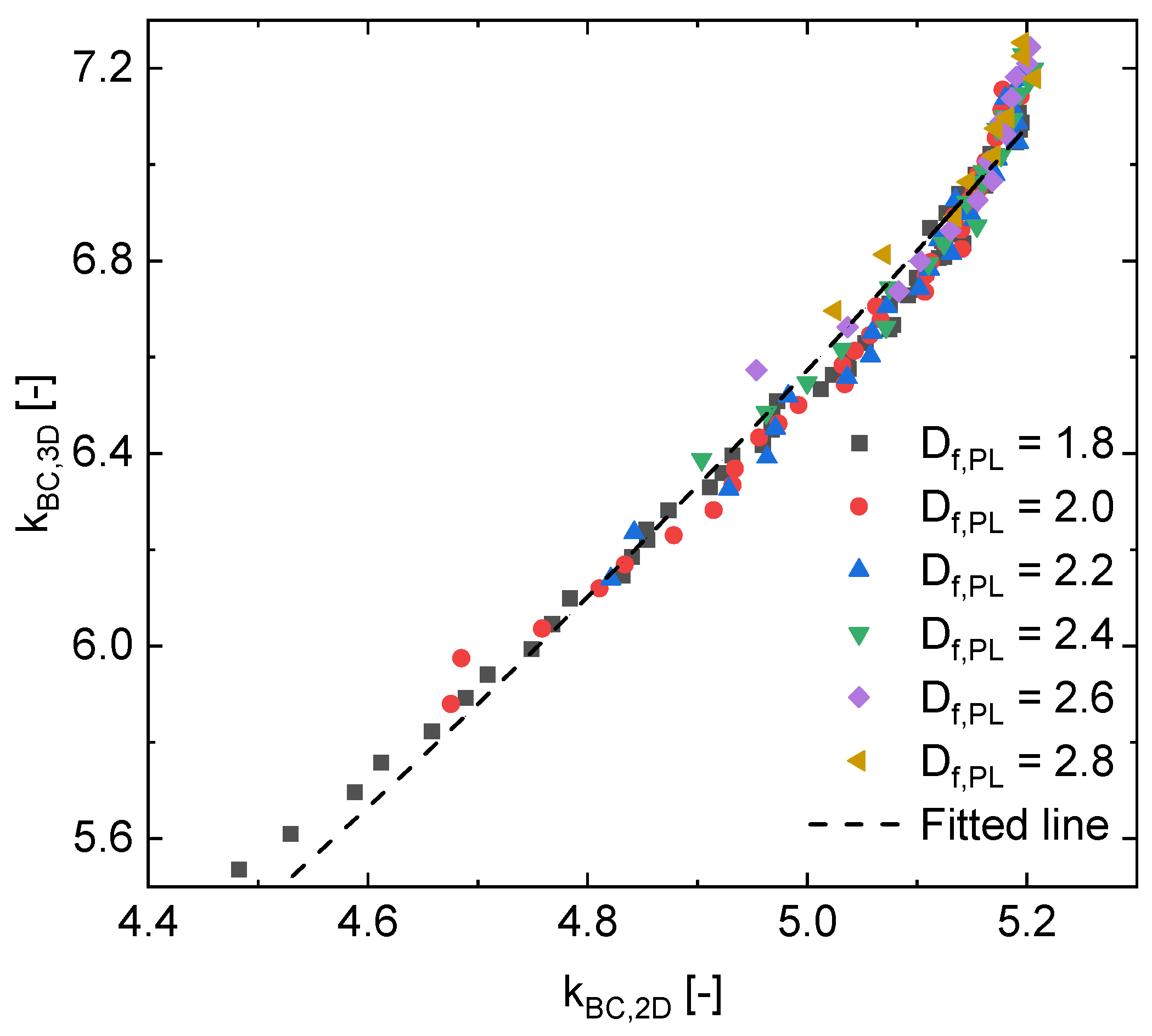
It is hard or even impossible to obtain the 3D fractal properties of aggregates composed of very small primary particles or nanoparticles by X-ray µ-CT, because of limitation in the spatial resolution of this imaging method. However, the 2D fractal properties of such aggregates can easily be retrieved by SEM or TEM. Therefore, a correlation between 2D and 3D fractal properties is necessary to be established. In this section, the correlation between 2D and 3D BC fractal properties is discussed first. Furthermore, the correlation between 2D BC and 3D PL fractal properties is discussed in the next section.
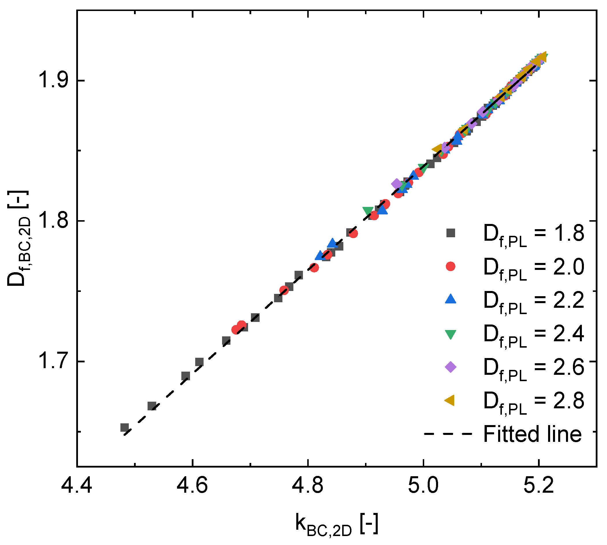
In
Figure 7, the relationship between
and
for the aggregates with various
(=1.8:0.2:2.8) is shown. Values of
and
have been averaged over all
(from 100 to 300 in steps of 50) of the entire aggregate series and then over five realizations.
As shown in
Figure 7,
increases with
for any value of power law fractal dimension. All data points can, thus, be described by one and the same power regression,
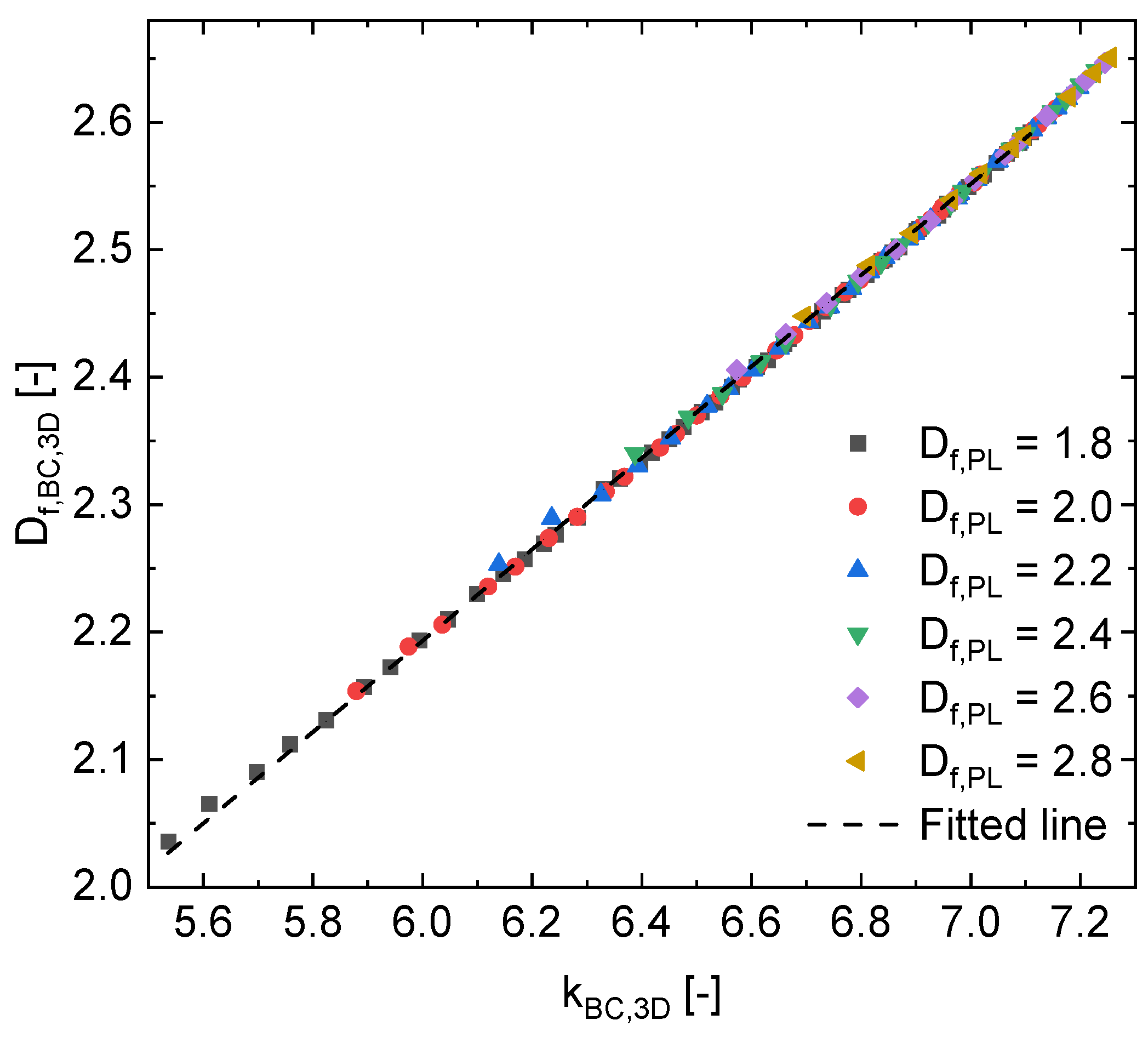
The average values of
(over five iterations) and
for the aggregates with different
are plotted in
Figure 8. From
Figure 8 we can find that the value of
is linearly increasing with
. The respective linear regression for all the aggregates is
A combination of Equations (11) and (12) can be used to obtain 3D BC fractal properties ( and ) from a given 2D BC prefactor or, by additionally involving the later Equation (17), from a given 2D BC fractal dimension .
3.4. Correlation between 2D BC Fractal Properties and PL Fractal Properties
The relationship between
and
for aggregates with various
(=1.8:0.2:2.8) is shown in
Figure 9. Values of
have been averaged over all
(from 100 to 300 in steps of 50) of the entire aggregate series and then over five realizations.
In
Figure 9,
is seen to increase with increasing
; however, the growth rate of
decreases as
increases. As pointed out in
Section 3.2, 2D BC fractal properties of aggregates are influenced by the 2D projection area [
28], being positively interrelated. And when the morphology of the aggregates with higher
or
has approached that of a sphere (as shown in
Figure 4), the projection area of these aggregates changes only slightly with further increase in
. Therefore, the rise of
with
flattens up at larger
or
. Here, an exponential function can be used for regression,
In Equation (13), the curves with different
have different values of
,
, and
, as summarized in
Table 6.
Then, correlations between, first,
and
, and second, between
and
are developed as follows:
The average value of = 5.208 is used to represent this parameter.
Combining Equations (13)–(15), the correlation between
and power law fractal properties is obtained:
The averages of
and
over five realizations are plotted in
Figure 10 for aggregates with different
. As shown in
Figure 10,
increases linearly with
, according to the regression
Equations (16) and (17) are very important. Combining these two equations enables to predict power law fractal properties ( and ) of aggregates from their 2D box-counting fractal properties ( and ), the determination of which from microscope images is fast and easy in practice.
Therefore, the reliability of these two correlations is tested by a new series of aggregates generated by the MPTSA model. Here, three different values of
are used, namely
= 1.9, 2.3, and 2.7. The input number of primary particles
varied from 100 to 300 in steps of 50. The prefactor
of the aggregates takes values from 0.9 to the upper limit of its effective range for each
(according to
Table 5). The primary particles are still monodispersed, and the radius of primary particles is kept same as for the previously generated aggregates. Each aggregate with the same input parameters is generated five times. Then, the aggregates that have been generated in 3D are projected onto a 2D plane by the projection method from [
28], and the 2D BC method is applied to estimate the 2D BC fractal properties for those projections. Then, the averages of
and
for each aggregate are calculated over five realizations. Substituting
and
into Equations (16) and (17), values of power law fractal properties (
and
) are finally calculated. Examples of calculated results for aggregates with
= 1.9 are summarized in
Table 7.
In
Table 7, there is a notable difference between the input fractal parameters and the calculated values. This is due to the difficult inversion of Equations (16) and (17) for given
and
. This is done by numerical optimization, which is though confronted with several flat and similar optima.
Whereas further improvement is desirable at this point, the ratio
, which is an important parameter for the morphological analysis of aggregates, can be applied to test the predicted values from Equations (16) and (17). It is recalled that Wang et al. [
28] have recently established an original correlation between 2D BC fractal dimension and PL fractal dimension. This correlation, however, neglected the influence of
and kept this parameter constant (=1). The correlation is
Predicted results (
and
) from Equations (16) and (17) are substituted to Equation (1) to calculate
of the new series of aggregates (
= 1.9, 2.3, and 2.7,
= 100, 200, and 300). For the sake of comparison,
of the new generated aggregates are substituted to Equation (18) to estimate their
. Then, keeping
as constant and equal to 1, another
is estimated by means of
predicted from Equation (18). Finally, the two kinds of
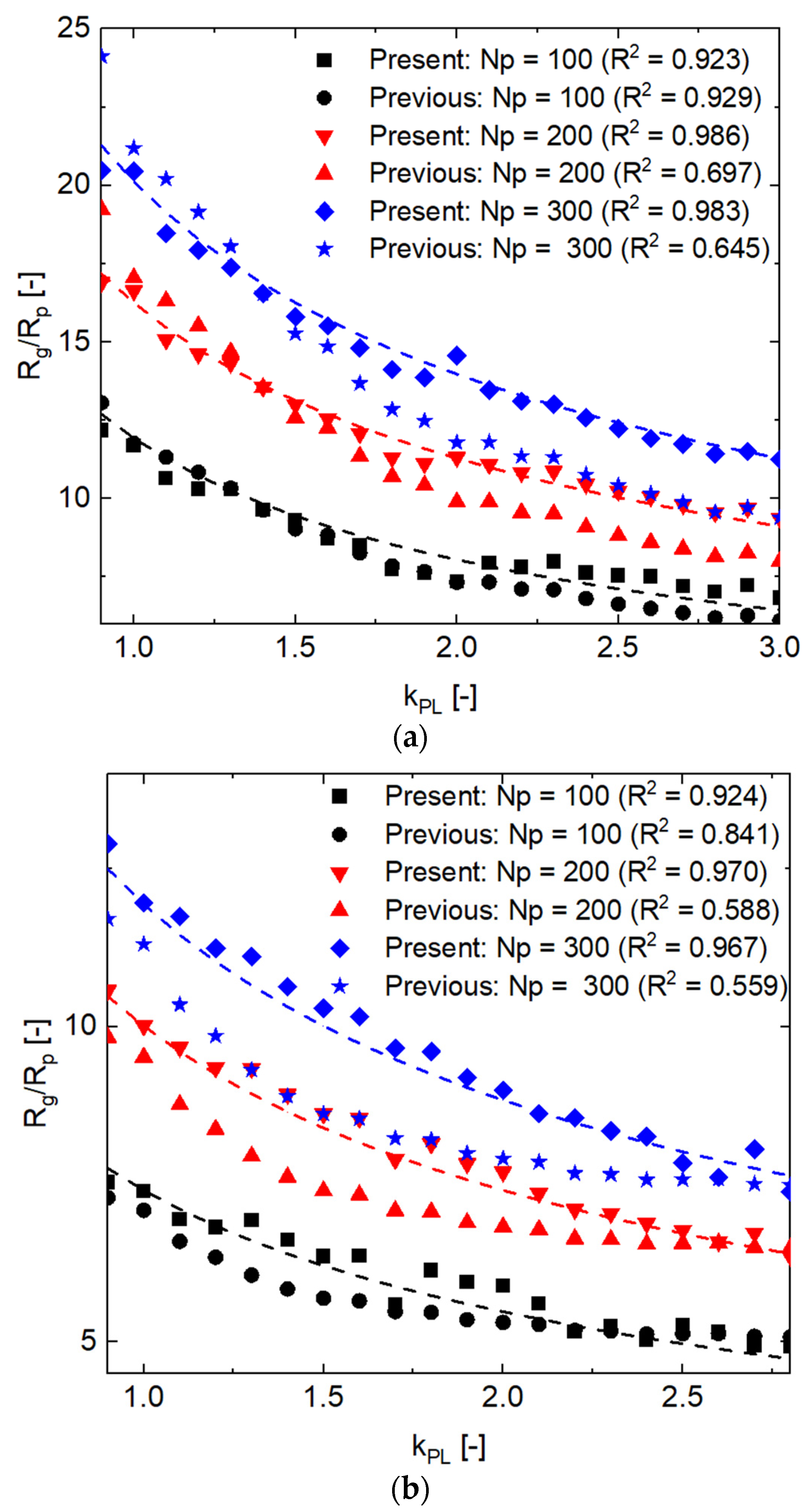
are compared in
Figure 11 based on three
(= 100, 200, and 300).
calculated from prediction results of the equations in this research (Equations (16) and (17)) are denoted by “present”,
calculated from the correlation of the previous work (Equation (18)) are denoted by “previous”. In addition, the standard
which is calculated from the input parameters (
,
, and
) of the MPTSA model is also shown in
Figure 11 (dotted lines). The R-square analysis represents the deviation of the predicted
(present or previous) to standard
.
As shown in
Figure 11, when both
and
are small (
= 1.9 and
= 100), the difference between present predicted results (Equations (16) and (17)) and previous predicted results (Equation (18)) is insignificant, the R
2 of the two sets of results to the standard (input, reference) data being 0.923 and 0.929, respectively. However, when
or
increases, the R
2 of previous results decreases significantly. Especially when the aggregates with
= 2.7 and
= 300 are considered, the R
2 of previous results reaches a very low value of 0.439. However, the changes in
or
hardly affect the accuracy of the present results, which are based on predictions from Equations (16) and (17). In
Figure 11, the minimum R
2 of present results is equal to 0.868 when
= 2.7 and
= 100.
