

Using a Fully Fractional Generalised Maxwell Model for Describing the Time Dependent Sinusoidal Creep of a Dielectric Elastomer Actuator


Abstract
1. Introduction
2. Materials and Methods
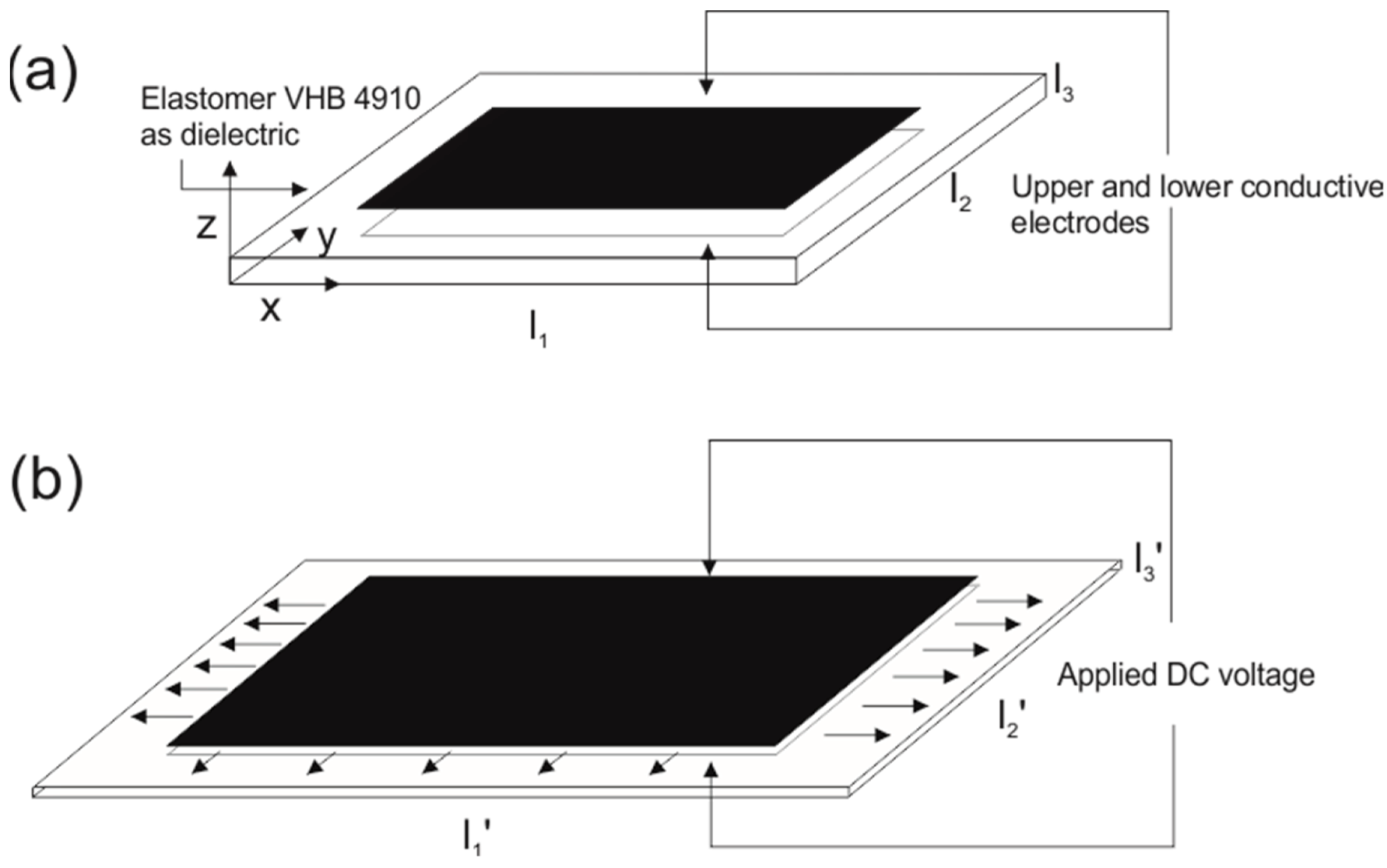
2.1. Principles of the DEA
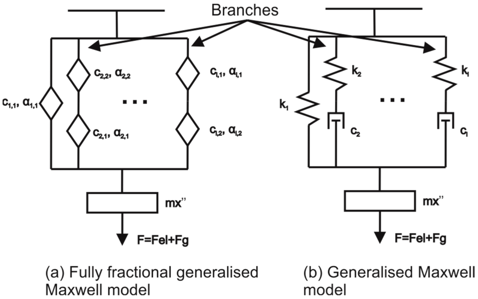
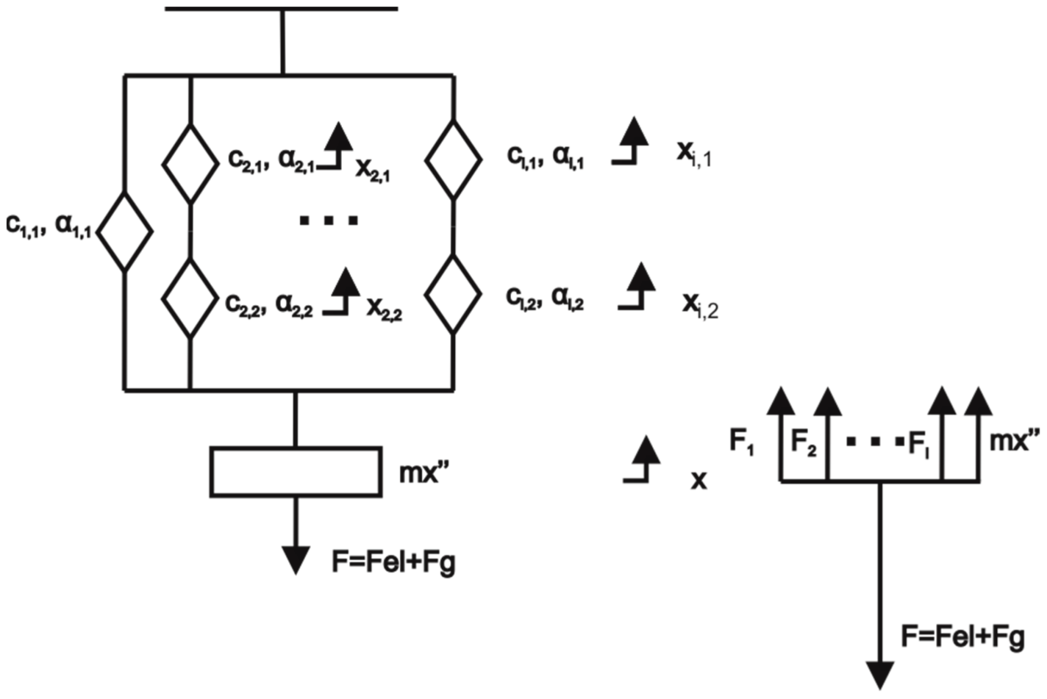
2.2. Derivation of the Fully Fractional Generalised Maxwell Model
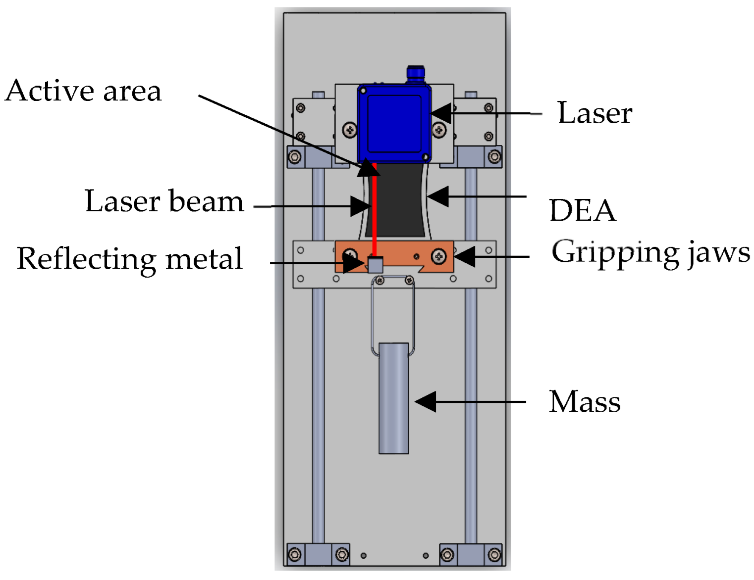
2.3. Experiments
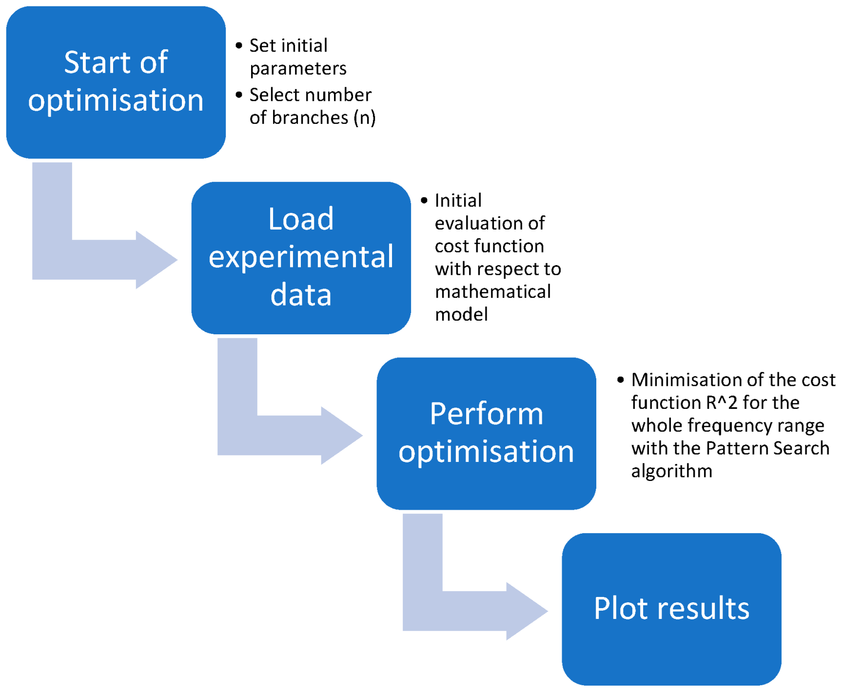
2.4. Optimisation
3. Results
4. Discussion
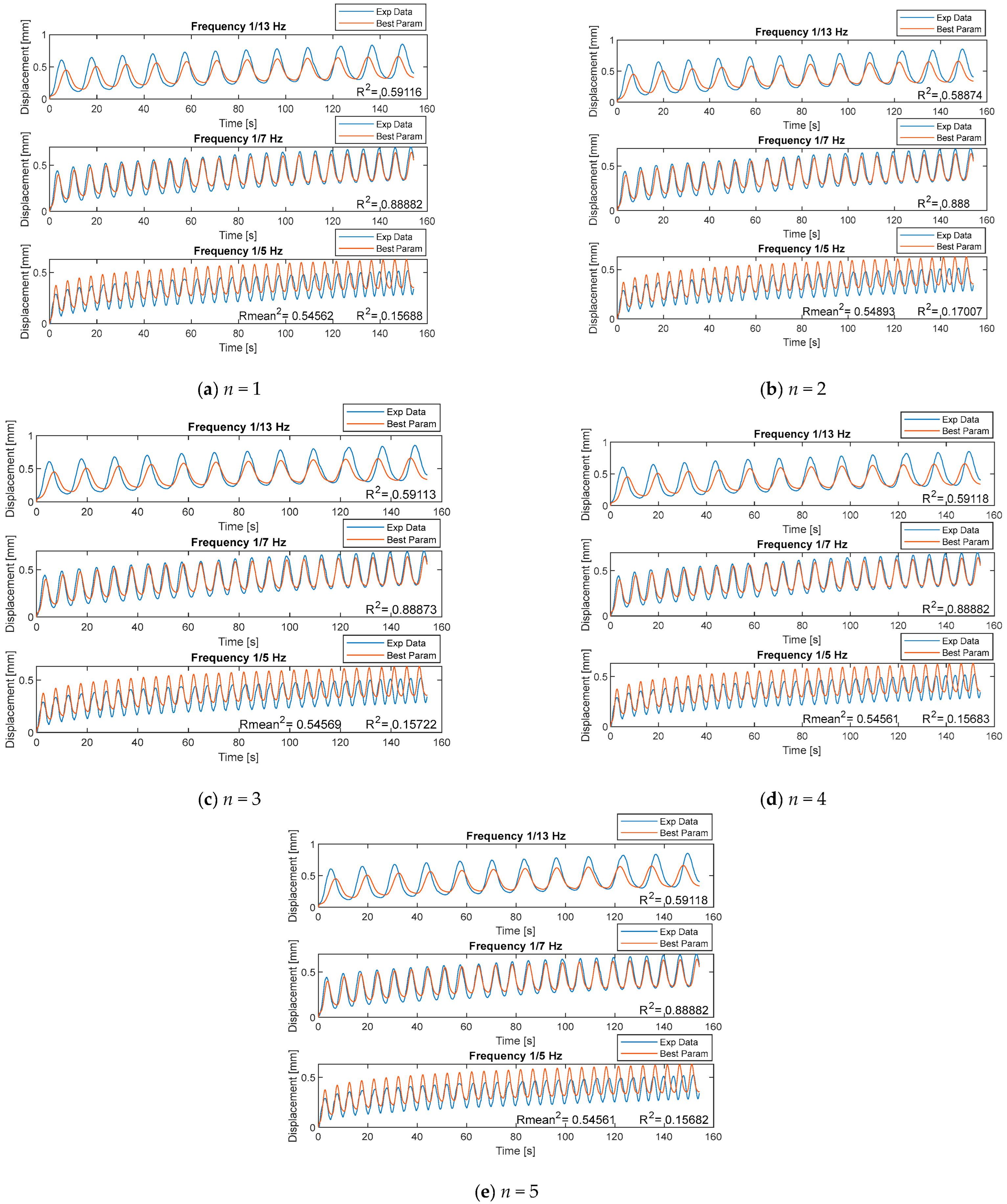
- The number of fully fractional Maxwell elements slightly affected the effectiveness of the model.
- Adding more than two branches did not increase the effectiveness of the model.
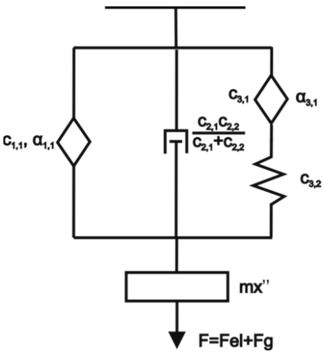
- The fully fractional Maxwell model was reduced to the model seen in Figure 8.
- The middle frequency of 1/7 Hz had the best agreement of 0.88 between data.
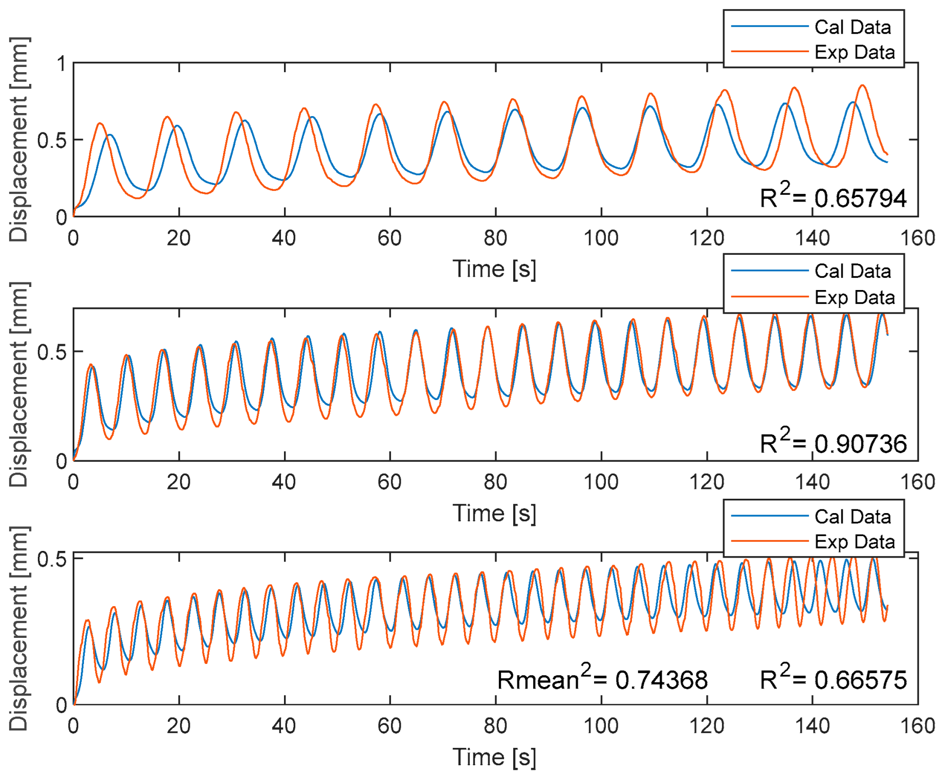
- Optimising each frequency individually drastically improved the overall agreement between data to 0.745.
- Optimising each frequency individually has a drawback since each frequency requires its own material parameters.
- Topology optimisation cannot be included into the Pattern Search algorithm.
5. Conclusions
Author Contributions
Funding
Data Availability Statement
Conflicts of Interest
References
- Youn, J.-H.; Jeong, S.M.; Hwang, G.; Kim, H.; Hyeon, K.; Park, J.; Kyung, K.-U. Dielectric Elastomer Actuator for Soft Robotics Applications and Challenges. Appl. Sci. 2020, 10, 640. [Google Scholar] [CrossRef]
- Bar-Cohen, Y. Electroactive Polymer (EAP) Actuators as Artificial Muscles: Reality, Potential, and Challenges; SPIE Press: Bellingham, WA, USA, 2001. [Google Scholar]
- Pei, Q.; Rosenthal, M.; Stanford, S.; Prahlad, H.; Pelrine, R. Multiple-degrees-of-freedom electroelastomer roll actuators. Smart Mater. Struct. 2004, 13, N86–N92. [Google Scholar] [CrossRef]
- Carpi, F.; Migliore, A.; Serra, G.; De Rossi, D. Helical dielectric elastomer actuators. Smart Mater. Struct. 2005, 14, 1210–1216. [Google Scholar] [CrossRef]
- Rui, Z.; Patrick, L.; Andreas, K.; Gabor, M.K. Spring roll dielectric elastomer actuators for a portable force feedback glove. In Proceedings of Smart Structures and Materials 2006: Electroactive Polymer Actuators and Devices (EAPAD), San Diego, CA, USA, 26 February–2 March 2006. [Google Scholar]
- Rosset, S.; Shea, H.R. Flexible and stretchable electrodes for dielectric elastomer actuators. Appl. Phys. A 2013, 110, 281–307. [Google Scholar] [CrossRef]
- Suo, Z.; Zhao, X.; Greene, W.H. A nonlinear field theory of deformable dielectrics. J. Mech. Phys. Solids 2008, 56, 467–486. [Google Scholar] [CrossRef]
- Gu, G.G.; Zhu, J.; Zhu, L.; Zhu, X. Modeling of Viscoelastic Electromechanical Behavior in a Soft Dielectric Elastomer Actuator. IEEE Trans. Robot. 2017, 133, 1263–1271. [Google Scholar] [CrossRef]
- Zou, J.; Gu, G. Modeling the Viscoelastic Hysteresis of Dielectric Elastomer Actuators with a Modified Rate-Dependent Prandtl–Ishlinskii Model. Polymers 2018, 10, 525. [Google Scholar] [CrossRef] [PubMed]
- Zou, J.; Gu, G. Dynamic modeling of dielectric elastomer actuators with a minimum energy structure. Smart Mater. Struct. 2019, 28, 085039. [Google Scholar] [CrossRef]
- Wissler, M.; Mazza, E. Mechanical behavior of an acrylic elastomer used in dielectric elastomer actuators. Sens. Actuators A Phys. 2007, 134, 494–504. [Google Scholar]
- Zhao, X.; Koh, S.; Suo, Z. Nonequilibrium Thermodynamics of Dielectric Elastomers. Int. J. Appl. Mech. 2011, 3, 203–217. [Google Scholar] [CrossRef]
- Xiang, G.; Yin, D.; Cao, C.; Gao, Y. Fractional description of creep behavior for fiber reinforced concrete: Simulation and parameter study. Constr. Build. Mater. 2022, 318, 126101. [Google Scholar] [CrossRef]
- Meng, R.; Yin, D.; Drapaca, C.S. Variable-order fractional description of compression deformation of amorphous glassy polymers. Comput. Mech. 2019, 64, 163–171. [Google Scholar] [CrossRef]
- Gao, Y.; Zhao, B.; Yin, D.; Yuan, L. A general fractional model of creep response for polymer materials: Simulation and model comparison. J. Appl. Polym. Sci. 2022, 139, 51577. [Google Scholar] [CrossRef]
- Su, X.; Chen, W.; Xu, W.; Liang, Y. Non-local structural derivative Maxwell model for characterizing ultra-slow rheology in concrete. Constr. Build. Mater. 2018, 190, 342–348. [Google Scholar]
- Xu, H.; Jiang, X. Creep constitutive models for viscoelastic materials based on fractional derivatives. Comput. Math. Appl. 2017, 73, 1377–1384. [Google Scholar] [CrossRef]
- Barretta, R.; Marotti de Sciarra, F.; Pinnola, F.P.; Vaccaro, M.S. On the nonlocal bending problem with fractional hereditariness. Meccanica 2022, 57, 807–820. [Google Scholar] [CrossRef]
- Luo, D.; Chen, H.-S. A new generalized fractional Maxwell model of dielectric relaxation. Chin. J. Phys. 2017, 55, 1998–2004. [Google Scholar] [CrossRef]
- 3M™. 3M™ VHB™ Tape Speciality Tapes. Available online: https://multimedia.3m.com/mws/media/986695O/3m-vhb-tape-specialty-tapes.pdf (accessed on 12 January 2021).
- Conductive, B. Electric Paint. Available online: https://www.bareconductive.com/shop/electric-paint-50ml/ (accessed on 11 July 2020).
- Podlubny, I. Fractional Differential Equations: An Introduction to Fractional Derivatives, Fractional Differential Equations, to Methods of Their Solution and Some of Their Applications; Elsevier Science: Amsterdam, The Netherlands, 1998. [Google Scholar]
- Mainardi, F. Fractional Calculus and Waves in Linear Viscoelasticity: An Introduction to Mathematical Models; Imperial College Press: London, UK, 2010; pp. 51–63. [Google Scholar]
- Mainardi, F.; Spada, G. Creep, relaxation and viscosity properties for basic fractional models in rheology. Eur. Phys. J. Spec. Top. 2011, 193, 133–160. [Google Scholar] [CrossRef]
- FOMCON. FOMCON Toolbox for Matlab. Available online: http://fomcon.net/ (accessed on 10 December 2020).
- Wenglor. YP05MGV80. Available online: https://www.google.com/url?sa=t&rct=j&q=&esrc=s&source=web&cd=1&ved=2ahUKEwihnaWa0bbjAhXiB50JHWepBx0QFjAAegQIBhAC&url=http%3A%2F%2Fwww.shintron.com.tw%2Fproimages%2Ftakex%2Fwenglor%2FYP05MGV80.pdf&usg=AOvVaw0hZdH3GNiqDLpm9BclkSVw (accessed on 15 July 2020).


| Symbol | Unit | Meaning |
|---|---|---|
| Area. | ||
| / | Order or fractional derivation of the springpots. | |
| Time limits of the fractional derivation. | ||
| Material properties of the springpots. | ||
| Modul of elasticity. | ||
| Absolute permittivity. | ||
| / | Relative permittivity. | |
| 1 | Strain. | |
| Maxwell force. | ||
| Electrical force. | ||
| Force in individual branch. | ||
| Calculated data. | ||
| / | Current number of fractional Maxwell element. | |
| Spring constant. | ||
| Dimensions of the DEA. | ||
| Initial length. | ||
| Displacement. | ||
| / | Integer order of derivation by the definition. | |
| Mass of weight. | ||
| / | Number of fractional Maxwell elements. | |
| Viscosity. | ||
| / | Fractional order of derivation by the definition. | |
| / | Coefficient of determination. | |
| / | Mean value of coefficient of determination. | |
| / | Laplace operator. | |
| / | Total sum of squares. | |
| / | Residual sum of squares. | |
| Stress. | ||
| Voltage. | ||
| Displacement of individual branch. | ||
| Measured data. | ||
| Averaged measured data. |
| Fully Fractional Generalised Maxwell Model Number of Branches | |
|---|---|
| n= 1 | 0.5456 |
| n= 2 | 0.5489 |
| n = 3 | 0.5456 |
| n = 4 | 0.5456 |
| n = 5 | 0.5456 |
| Param. | n= 1 | |||||||||||
| Initial | 0.2 | 1 | 1 | |||||||||
| Optimised | 0.2 | 0.002 | 1 | |||||||||
| Parameters | ||||||||||||
| Initial | 500 | 500 | 500 | |||||||||
| Optimised | 62.952 | 0.036 | 0.142 | |||||||||
| Param. | n= 2 | |||||||||||
| Initial | 0.2 | 1 | 1 | 1 | 1 | |||||||
| Optimised | 0.2 | 1 | 1 | 0.523 | 0.046 | |||||||
| Param. | ||||||||||||
| Initial | 500 | 500 | 500 | 500 | 500 | |||||||
| Optimised | 62.740 | 47.958 | 173.21 | 430.381 | 0.215 | |||||||
| Param. | n= 3 | |||||||||||
| Initial | 0.2 | 1 | 1 | 1 | 1 | 1 | 1 | |||||
| Optimised | 0.2 | 1 | 1 | 1 | 0.002 | 1 | 1 | |||||
| Param. | ||||||||||||
| Initial | 500 | 500 | 500 | 500 | 500 | 500 | 500 | |||||
| Optimised | 62.950 | 0.267 | 0.464 | 0.140 | 0.088 | 0.036 | 0.237 | |||||
| Param. | n= 4 | |||||||||||
| Initial | 0.2 | 1 | 1 | 1 | 1 | 1 | 1 | 1 | 1 | |||
| Optimised | 0.2 | 0.002 | 1 | 0.002 | 1 | 1 | 0.002 | 1 | 0.002 | |||
| Param. | ||||||||||||
| Initial | 500 | 500 | 500 | 500 | 500 | 500 | 500 | 500 | 500 | |||
| Optimised | 62.950 | 0.103 | 0.036 | 0.321 | 0.036 | 0.094 | 0.157 | 0.036 | 0.225 | |||
| Param. | n= 5 | |||||||||||
| Initial | 0.2 | 1 | 1 | 1 | 1 | 1 | 1 | 1 | 1 | 1 | 1 | |
| Optimised | 0.2 | 0.002 | 1 | 1 | 1 | 1 | 0.002 | 1 | 0.002 | 1 | 1 | |
| Param. | ||||||||||||
| Initial | 500 | 500 | 500 | 500 | 500 | 500 | 500 | 500 | 500 | 500 | 500 | |
| Optimised | 62.950 | 0.097 | 0.315 | 0.036 | 0.356 | 0.036 | 0.097 | 0.036 | 0.095 | 0.036 | 0.285 |
| Parameters | F = 1/13 Hz n = 3 | ||||||||
| Initial | 0.2 | 1 | 1 | 1 | 1 | ||||
| Optimised | 0.1795 | 1 | 1 | 1 | 1 | ||||
| Parameters | |||||||||
| Initial | 500 | 500 | 500 | 500 | 500 | 0.658 | |||
| Optimised | 51.773 | 0.002 | 0.002 | 0.002 | 0.002 | ||||
| Parameters | F = 1/7 Hz n = 3 | ||||||||
| Initial | 0.2 | 1 | 1 | 1 | 1 | ||||
| Optimised | 0.188 | 0.255 | 0.046 | 0.225 | 0.880 | ||||
| Parameters | |||||||||
| Initial | 500 | 500 | 500 | 500 | 500 | 0.907 | |||
| Optimised | 57.696 | 569.346 | 0.003 | 406.744 | 0.479 | ||||
| Parameters | F = 1/5 Hz n = 3 | ||||||||
| Initial | 0.2 | 1 | 1 | 1 | 1 | ||||
| Optimised | 0.2 | 1 | 1 | 1 | 0.002 | ||||
| Parameters | |||||||||
| Initial | 500 | 500 | 500 | 500 | 500 | 0.665 | |||
| Optimised | 73.133 | 19.199 | 188.074 | 305.285 | 191.367 | ||||
| 0.743 |
Publisher’s Note: MDPI stays neutral with regard to jurisdictional claims in published maps and institutional affiliations. |
© 2022 by the authors. Licensee MDPI, Basel, Switzerland. This article is an open access article distributed under the terms and conditions of the Creative Commons Attribution (CC BY) license (https://creativecommons.org/licenses/by/4.0/).
Share and Cite
Karner, T.; Belšak, R.; Gotlih, J. Using a Fully Fractional Generalised Maxwell Model for Describing the Time Dependent Sinusoidal Creep of a Dielectric Elastomer Actuator. Fractal Fract. 2022, 6, 720. https://doi.org/10.3390/fractalfract6120720
Karner T, Belšak R, Gotlih J. Using a Fully Fractional Generalised Maxwell Model for Describing the Time Dependent Sinusoidal Creep of a Dielectric Elastomer Actuator. Fractal and Fractional. 2022; 6(12):720. https://doi.org/10.3390/fractalfract6120720
Chicago/Turabian StyleKarner, Timi, Rok Belšak, and Janez Gotlih. 2022. "Using a Fully Fractional Generalised Maxwell Model for Describing the Time Dependent Sinusoidal Creep of a Dielectric Elastomer Actuator" Fractal and Fractional 6, no. 12: 720. https://doi.org/10.3390/fractalfract6120720
APA StyleKarner, T., Belšak, R., & Gotlih, J. (2022). Using a Fully Fractional Generalised Maxwell Model for Describing the Time Dependent Sinusoidal Creep of a Dielectric Elastomer Actuator. Fractal and Fractional, 6(12), 720. https://doi.org/10.3390/fractalfract6120720