Article

Fractal Continuum Calculus of Functions on Euler-Bernoulli Beam

1
SEPI-ESIME Zacatenco, Instituto Politécnico Nacional, Unidad Profesional Adolfo López Mateos, Mexico City 07738, Mexico
2
Engineering Department, Instituto Politécnico Nacional, UPIITA, Av. IPN, No. 2580, Col. La Laguna Ticoman, Gustavo A. Madero, Mexico City 07340, Mexico
*
Author to whom correspondence should be addressed.
Fractal Fract. 2022, 6(10), 552; https://doi.org/10.3390/fractalfract6100552
Submission received: 19 July 2022 / Revised: 21 September 2022 / Accepted: 27 September 2022 / Published: 29 September 2022
(This article belongs to the Special Issue Fractal Approaches in Materials: Structure and Mechanics)

Abstract

:
A new approach for solving the fractal Euler-Bernoulli beam equation is proposed. The mapping of fractal problems in non-differentiable fractals into the corresponding problems for the fractal continuum applying the fractal continuum calculus ( F d H 3 -CC) is carried out. The fractal Euler-Bernoulli beam equation is derived as a generalization using F d H 3 -CC under analogous assumptions as in the ordinary calculus and then it is solved analytically. To validate the spatial distribution of self-similar beam response, three different classical beams with several fractal parameters are analysed. Some mechanical implications are discussed.

1. Introduction

Fractal geometry has been widely used in many fields of science and technology such as: medicine [1,2], hydrology [3,4], materials science [5,6,7], applied physics [8,9] and mathematical modelling [10,11,12], among others.
The concept of fractal continuum was introduced in 2005 by Tarasov [13] and has become popular in the last two decades. Many different methods of nonlocal and local fractal continua have been formulated [14,15,16,17,18,19,20,21,22,23,24,25,26].
In this regard, the fractal continuum calculus, introduced by Balankin and Elizarraraz [20,21], gives possibility to define generalized differential structures, which are non-differentiable in ordinary sense. This formulation was validated on fractal materials to solve the pressure-transient and Maxwell Equations [21,23]. Recently, this method was applied to derive the fractal Euler-Bernoulli beam equation using the virtual work principle [27].
In [22,28], fractal continuum calculus was firstly formulated based on classical Menger sponge embedded in 3 . Main definitions involve the assumption of a fractal continuum F d H 3 without pores or empty spaces defined as a three-dimensional object in 3 and endowed with appropriate fractional measure, metric, and norm and a set of rules for integro-differential calculus, as well as with a proper Laplacian, accounting for the metric, connectivity, and topological properties of the fractal domain [28].
This concept enables us to map the fractal domain denoted by F 3 d H 3 (see Figure 1), whose properties are essentially discontinuous in the embedding space 3 , into the fractal continuum domain denoted by F d H 3 3 (see Figure 2), the properties of which behave as analytic envelopes of non-analytic functions in the fractal object under study [20,21]. The generalization from F 3 d H to F d H 3 using local fractional differential operators is called fractal continuum calculus F d H 3 -CC, and it has been adopted in order to solve different engineering problems [20,23,27].
The present manuscript shows applications of fractal Euler-Bernoulli equation using F d H 3 -CC to calculate the spatial distribution of rotation and transversal displacement in classical beams with fractal geometry. The generalization from ordinary calculus to fractal continuum calculus of Euler-Bernoulli beam equation is carried out using the engineering mechanics approach based mainly on two assumptions: the constitutive law of isotropic elasticity and the geometry of deformation [29], as an alternative approach to the principle of virtual work. The total mechanical response caused by the fractal configuration of the self-similar beams is highlighted.
The paper consists of 5 sections: following the "Introduction", we review the basic tools required in Section 2. Whereas Section 3 is devoted to the formulation of fractal Euler-Bernoulli beam equation. Proposed formulation is applied to classical beams and the structural details are discussed in Section 4. Section 5 closes the paper with conclusions.

2. Mathematical Background

First, we review Menger’s sponge-like sets and their properties and then we summarize F d H 3 -CC.

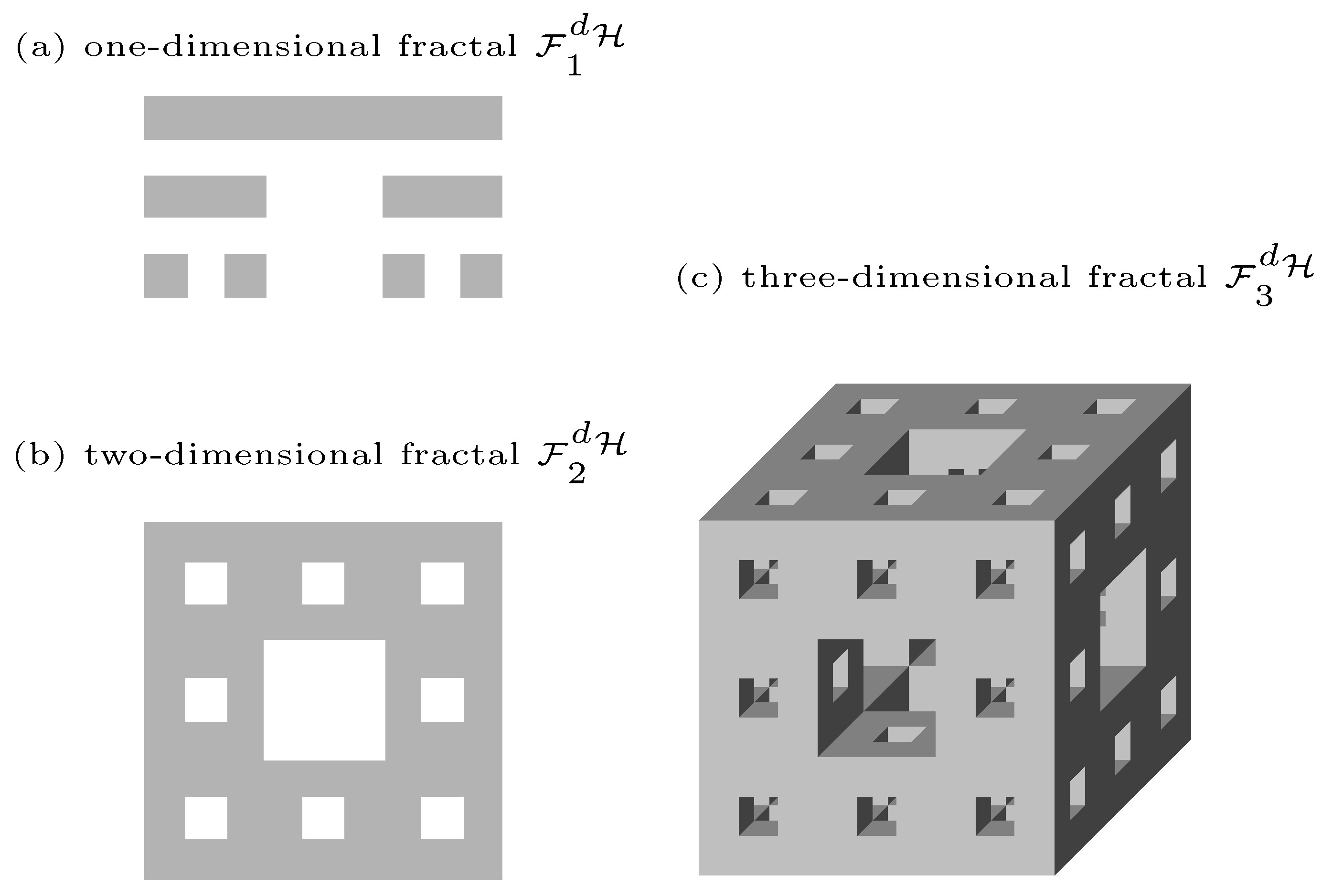
2.1. Menger Sponge Fractals
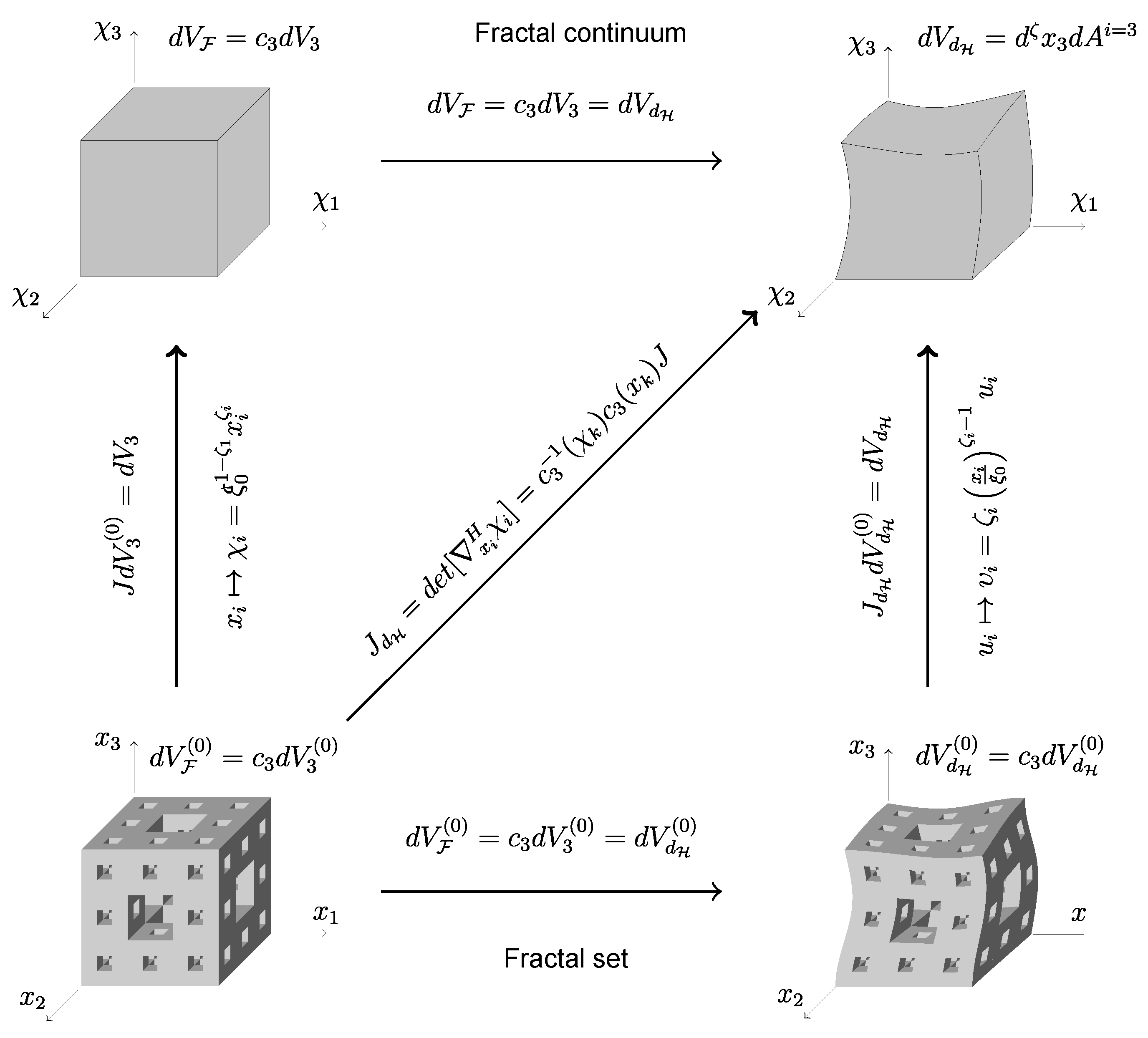
The Menger sponge M η is a three-dimensional version of the middle- η Cantor fractal set C η [ 0 , 1 ] and the Sierpinski carpet S η is its two-dimensional version (see Figure 1), which are self-similar fractals.
The middle- η Cantor set C η is constructed by iterative removal of open middle- η segments from remaining segments of the previous iteration, starting from the unit interval [ 0 , 1 ] = L (divided in segments of size 0 < η < 1 ) ad infinitum [30].
In similar fashion, the Sierpinski carpet can be constructed by iterative process from the unit square [ 0 , 1 ] 2 , which is divided into η × η sub-squares of equal size and the interior of β 2 sub-squares are deleted. Iterating this process infinitely many times we obtain the fractal S η [ 0 , 1 ] 2 2 .
Finally, the Menger sponge is constructed starting from the unit cube [ 0 , 1 ] 3 3 , which is divided into η × η × η sub-cubes of equal size, after that, the interior of β 3 sub-cubes are deleted. In each of the remaining sub-cubes the same operation is repeated. This procedure is iterated ad infinitum (see Figure 1).
Figure 1. Construction of three-dimensional fractal Menger sponge, (a) The middle- 1 / 3 Cantor set: C 1 / 3 , (b) two-dimensional Cantor Set or Sierpinski carpet: S 1 / 3 2 , and (c) three-dimensional Cantor set or Menger sponge: M 1 / 3 3 .
Fractalfract 06 00552 g001
Hausdorff dimension of the above fractals is given by [31]:
d H = log η n β n log η ,
where the value of d H is constant for ξ 0 < L ξ C , where ξ 0 and ξ C are the lower and upper cutoffs, respectively [32]; η = L / ξ 0 denotes the size of box needed to cover the fractal mass, β is the total number of boxes removed from the fractal mass and n = 1 , 2 , 3 , defines the Hausdorff dimension for the one, two and three-dimensional versions of Cantor middle- η , respectively [27,31].
The connectivity and topology of Menger sponge are characterized by the chemical fractal dimension d , as any fractal F 3 d H can be covered by d -dimensional boxes [33] of size at most L / ξ , such that [33]:
d = log N L ξ log L ξ .
The above equation implies that ξ is measured with respect to the geodesic metric on M η [34]. From Equations (1) and (2) it follows that ξ d ξ 0 d H such that, the geodesic distances between two points on the fractal L g scales with the Euclidean distance between these points in the embedding Euclidean space L as L g L d g , being d g = d H / d = 1 the geodesic dimension of Menger sponge [34]. Another characteristics of the fractal topology are the fractal dimensions of cross-section areas d A i given by the intersections between the fractal domain F 3 d H 3 and two-dimensional Cartesian planes in 3 [20,21], where the index i = 1 , 2 , 3 denotes the Cartesian plane orthogonal to i-axis. Fractal area of cross section d A scales with its linear size L and so, for the Menger sponge where η = 1 / 3 we have that 2 d = d H = 2.72 3 and A F is defined as [27,28]:
A F = ξ 0 2 L ξ 0 d A ;
where d A = d H ( S 1 / 3 ) = 1.89 . On the other hand, the fractal distance on x i ( L ) is given by [28]:
x i ( L ) = ξ 0 L ξ 0 ζ i ,
where
ζ i = d H d A
is the fractal dimension of the coordinate χ i . Meanwhile, the fractal mass M scales with respect to the linear size L ( ξ 0 , ξ C ) as [13]:
M = ρ 0 x i ( L ) A F = ρ 0 ξ 0 3 L ξ 0 d H ,
where ρ 0 is the mass density.
The fractal measure of M η is characterized by its Hausdorff dimension d H , whereas the fractal metric is controlled by the fractal dimension of the coordinate χ i given by ζ i = d H d A i along with the chemical dimension d .

2.2. Mapping F 3 d H F d H 3

The F d H 3 -CC consists in to make an approximation of non-differentiable functions defined on fractals F 3 d H by differentiable analytic envelopes into fractal continuum F d H 3 in the fractal object under study [20,21,28]. For this reason, F d H 3 3 is defined as a three-dimensional region filled with continuous matter and so, its topological dimension is d t = 3 . In addition, it was endowed with the following local fractional differential operators [28]:
i
Fractional norm is given by A = i 3 χ a i 2 γ 1 / 2 γ , being γ = d / 3 1 and
χ i = ξ 0 1 ζ i x i ζ i
are the fractional coordinates in fractal continuum domain F 3 d H 3 allied with the Cartesian coordinates in n (for i = 1 , 2 , 3 ).
ii
Distance between two points A , B F 3 d H is given by Δ ( A , B ) = i 3 Δ i 2 γ 1 / 2 γ being Δ i = χ a i χ b i .
iii
Local partial derivatives in F d H 3 3 so-called Hausdorff derivatives [28] can be expressed in terms of conventional partial derivatives ( / x i ) in 3 as:
i H f = lim χ i χ i f ( χ i ) f ( χ i ) χ i χ i = lim x i x i f ( x i ) f ( x i ) Δ x i , x i = χ i f ( χ i ) = 1 c 1 i x i f
where c 1 i = ζ i ξ 0 1 ζ i x i ζ i 1 is the density of admissible states along the i-axis in F d H 3 3 .
iv
Hausdorff del operator in F d H 3 is defined as H = e 1 1 ζ + e 2 2 ζ + e 3 3 ζ , where e i 3 are basis vectors.
v
The divergence is given by:
d i v H f = i 3 1 c 1 i f x i ,
vi
And the generalized Laplacian of scalar function is defined as:
Δ H F f = i H · i H f = i 3 c 1 i 2 2 f x i 2 + γ ζ i x i f x i
while the infinitesimal volume element in F d H 3 3 can be generally decomposed as:
d V d H = d χ i ( x i ) d A i ( x j i ) = c 1 i ( x i ) c 2 i ( x j i ) d x i d A 2 i = c 3 ( x k ) V 3 = c 3 d x 1 d x 2 d x 3
where d A 2 i = d x j d x k and d A i are the infinitesimal area elements on the intersection between F d H 3 and two-dimensional plane normal to i-axis in 3 and in F d H 3 3 , respectively, c 2 i ( x j i ) is the density of admissible states in the plane of this intersection, and c 3 = c 1 i c 2 i .
vii
The measure in the fractal continuum is defined by the following relations d V 3 c 3 ξ 0 3 d H L d H , d A 2 i c 2 i L d A i and d χ i = d x i c 1 i ξ 0 1 ζ i L ζ i .
On the other hand, the concept of elastic fractal continuum is governed by the Equations [27]
d i v H σ i j + b i = 0 , ε i j = 1 2 j H υ i + i H υ j = 1 2 1 c 1 υ i x j + υ j x i , σ i j = C i j k l ε k l , u i = u ^ i , σ i j n j = t ^ i ,
where σ i j is the Cauchy stress tensor and b i is the body force; ε i j is the infinitesimal strain tensor; C i j k l is the stiffness tensor; n j is the outward unit normal vector; t is the Cauchy traction vector; x is a material variable, u is the displacement and Ω u and Ω σ are parts of boundary F d H 3 where the displacements and the tractions are applied, respectively. We have c 1 = ζ 1 x 1 / ξ 0 ζ 1 1 , and υ i F d H 3 are defined by [28] as:
υ i = ζ i x i ξ 0 ζ i 1 u i
where υ i are the components of the displacement vector in fractal continuum domain. In Figure 2 the relations between initial and deformed configurations on the mapping from a fractal set to its corresponding fractal continuum, F 3 d H F d H 3 are presented.
Figure 2. Geometrical interpretation of mapping of Menger sponge F 3 2.72 into the fractal continuum F 2.72 3 from the original to deformed configurations [22,28].
Fractalfract 06 00552 g002

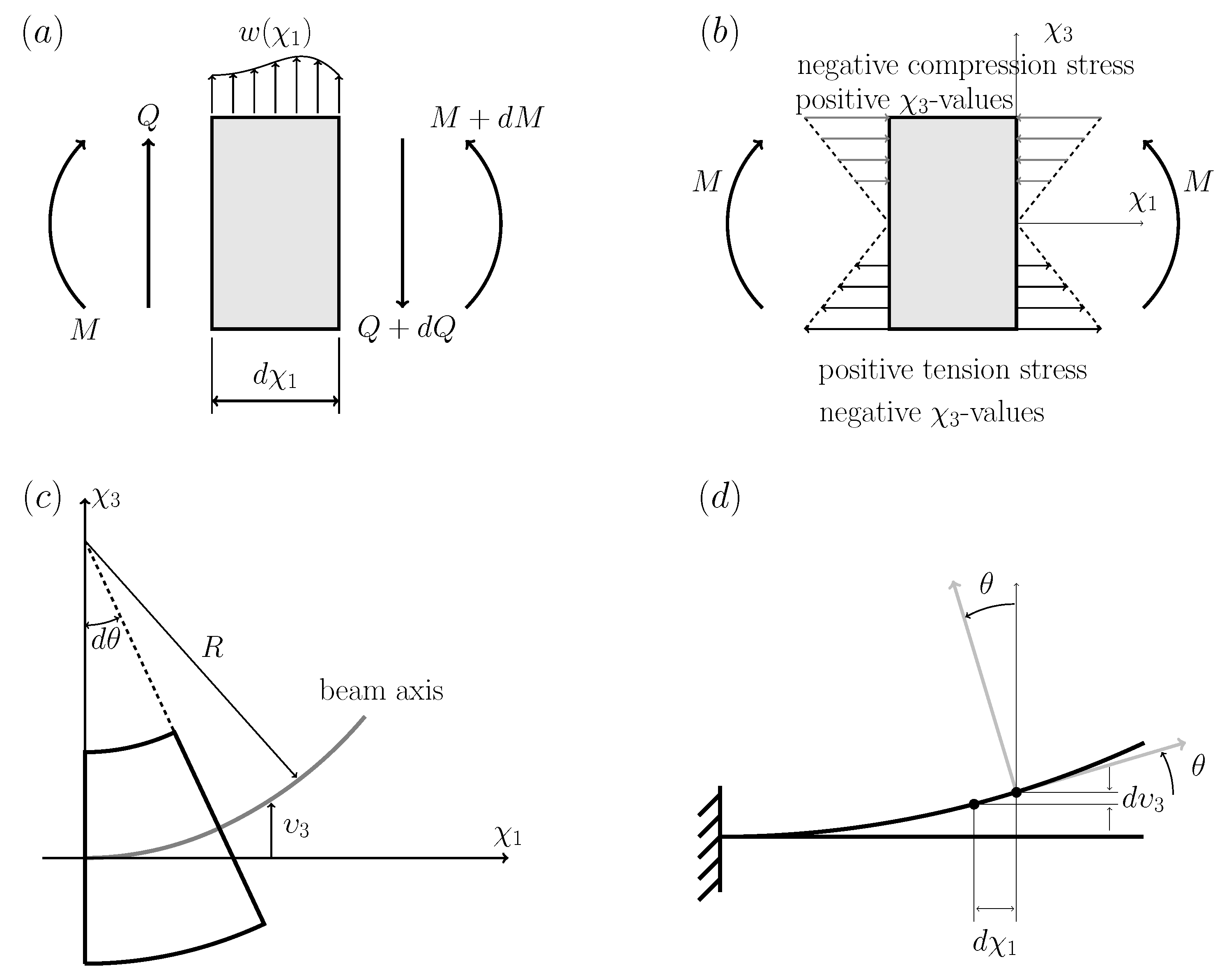
3. Differential Equations of Euler-Bernoulli Beam Using F d H 3 -CC

This section is devoted to deduce the Euler-Bernoulli beam equation for fractal beams by applying concepts reviewed in the behold section.
The fractal Euler-Bernoulli beam theory is based on the following assumptions [35]:
1.
The cross-section is infinitely rigid in its own plane. This implies there is no deformations in the plane of the cross-section.
2.
The cross-section of a beam remains plane after deformation: a transverse plane section perpendicular to the centroidal axis of the beam before deformation remains plane after bending.
3.
The cross-section remains normal to the deformed axis of the beam, i.e., the cross section is perpendicular to the bent centroidal axis after bending.
Governing equations of the Euler-Bernoulli beam in the mechanics of fractal continuum are obtained under the analogous assumptions like those obtained in classical calculus.
Considering an infinitesimal beam element as is shown in Figure 3a, the following equilibrium equations can be obtained, for the vertical equilibrium:
w ( χ 1 ) = d Q d χ 1 ,
and for the moment equilibrium:
Q = d M d χ 1 ,
On the other hand, the bending moment M is deduced by the integration of axial stresses over the cross section as
M = A σ χ 3 d A ,
for a geometrical illustration see the Figure 3b. Whereas that the relationship between the axial strain and the transversal displacement of a beam element is given by
ε = d υ 1 d χ 1 .
In Figure 3c an infinitesimal beam element is plotted where it can be observed that the axial displacement υ 1 is related to the rotation θ of the cross-section. It is a straightforward matter to see the axial displacement of each infinitesimally short fibre is
d υ 1 = d θ χ 3 .
Finally, the rotation θ is related to the transversal displacement υ 3 . The geometrical interpretation of Figure 3d, shows that
tan θ = d υ 3 d χ 1 θ ,
which is possible because the deformations are sufficiently small so that tan θ θ . So, the kinematics equation for the beam members is obtained as
ε = d υ 1 d χ 1 = d θ d χ 1 χ 3 = d 2 υ 3 d χ 1 2 χ 3 .
This expression implies an approximation of the exact curvature of the beam. Mathematically, the curvature is defined as κ = 1 / R , where R is the radius of curvature of the beam. In the Euler-Bernoulli beam theory that is presented here, the curvature is approximated by κ = d θ / d χ 1 d 2 υ 3 / d χ 1 2 (see Figure 2).
The differential equation for the beam bending is obtained substituting Equation (16) in Equation (15) and substituting the result in Equation (14), so:
w ( χ 1 ) = d Q d χ 1 = d 2 M d χ 1 2 = d 2 d χ 1 2 A σ χ 3 d A ,
by applying the Hooke law σ = E ε and Equation (20) in the above equation, we obtain
w ( χ 1 ) = d 2 d χ 1 2 A E ε χ 3 d A = E d 2 d χ 1 2 d 2 υ 3 d χ 1 2 A χ 3 2 d A = E I d 4 υ 3 d χ 1 4 ,
where A χ 3 2 d A = I defines the moment of inertia. Then, the governing Equation (22) that relates the deflection with the load applied to beam is obtained.
The generalization of Equations (19) and (22) from ordinary calculus to fractal continuum calculus is carried out using Equations (7) and (13) in order to map the fractal beam into fractal continuum beam, so the fractal rotation is
θ ( χ 1 ) = d υ 3 d χ 1 = ξ 0 ζ 1 1 d u 3 d x 1 ζ 1 ,
and for the fractal Euler-Bernoulli bending beam
w ( χ 1 ) = E I d 4 υ 3 d χ 1 4 = ξ 0 4 ζ 1 4 E I d 4 u 3 d x 1 4 ζ 1 .
It is worth noting that for ζ i = 1 , the fractal Euler-Bernoulli beam equation takes the form of the ordinary equation of Euler-Bernoulli beam w ( x 1 ) = E I d 4 u 3 / d x 1 4 . Moreover, the generalized Euler-Bernoulli bending equation is valid only if the bending moment acts on one of the principal axes of the cross-section and the bending axis acts on a symmetric cross-section; otherwise, combined bending occurs in both principal axes of the cross-section. Therefore, this restriction must be taken into account when applying Euler-Bernoulli’s bending theory. The resultant axial force on the cross-sectional area is equal to zero only when the neutral axis passes through the centroid of the area, such that A σ d A = 0 .

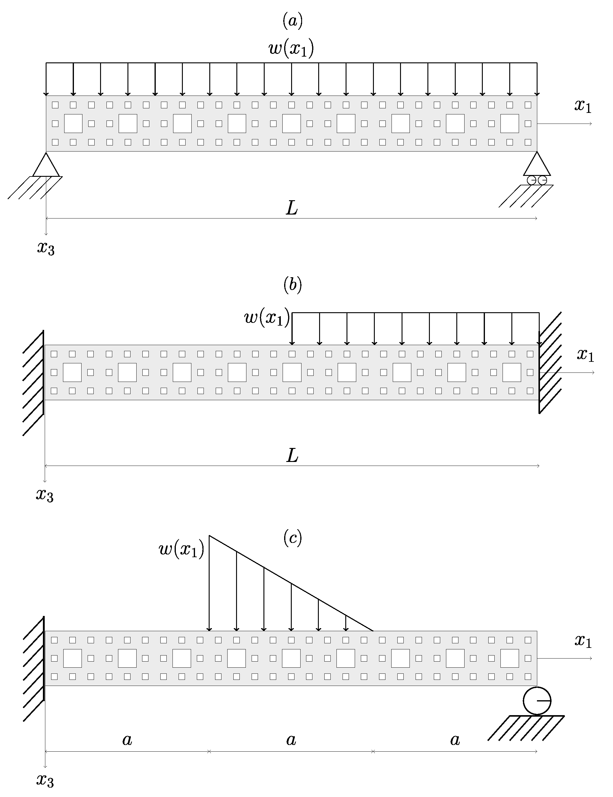
4. Bending of Self-Similar Beams

In this section we apply the fractal Euler-Bernoulli equation on classical beams with different fractal geometry and several boundary conditions in order to demonstrate its engineering implications.

4.1. Illustrative Examples

We consider three different beams presented in Figure 4. The fractal parameters of the beams are given in Table 1; where η represents the mass removed in the corresponding Cantor set from which the Sierpinski carpet and Menger sponge are constructed, i.e., for the triadic Cantor set ( η = 1 / 3 ), the classical Sierpinsky carpet and Menger sponge are obtained (see Figure 1); while for η = 0 , the corresponding Cantor set is the unitary interval [ 0 ,   1 ] , consequently, the Hausdorff dimension of Sierpinski carpet is two and the Menger sponge has d H = 3 , and the beam is a Euclidean solid beam. The beam is self-similar for all cases where η > 0 (see Figure 4). Besides, each beam has the following data: L = 2.7 m, h = b = 0.3 m, a = L / 3 , E = 30 × 10 9 N/m 2 , w = 100 N/m.
For the simply supported beam the structural analysis is carried out with the following boundary conditions:
υ 3 ( 0 ) = M ( 0 ) = υ 3 ( L ) = M ( L ) = 0 .
Meanwhile for the fixed cantilever beam the boundary conditions are:
υ 3 ( 0 ) = θ ( 0 ) = υ 3 ( L ) = θ ( L ) = 0 ,
and for the propped beam we have:
υ 3 ( 0 ) = θ ( 0 ) = υ 3 ( L ) = M ( L ) = 0 ,

4.2. Fractal Response Details

By applying boundary conditions given in Equations (25)–(27) the transversal displacement and rotation for the classical beams studied are obtained:
Simply supported beam. The transversal displacement in fractal coordinates is given by:
υ 3 ( χ 1 ) = w χ 1 24 E I χ 1 3 2 L χ 1 2 + L 3
and the map from F 3 d H into F d H 3 for the displacement is:
υ 3 ( χ 1 ) = w ξ 0 4 4 ζ 1 x 1 ζ 1 24 E I x 1 3 ζ 1 2 L ζ 1 x 1 2 ζ 1 + L 3 ζ 1 .
Fixed beam. This beam has two ranges
υ 3 ( χ 1 ) = w E I 5 L 2 384 χ 1 2 + 3 L 192 χ 1 3 , for 0 < χ 1 L 2 w E I 5 L 2 384 χ 1 2 + 3 L 192 χ 1 3 1 24 χ 1 L 2 4 , for L 2 < χ 1 < L
and the fractal displacement in Cartesian coordinates is described by
υ 3 ( χ 1 ) = w ξ 0 4 4 ζ 1 E I 5 L 2 ζ 1 384 x 1 2 ζ 1 + 3 L ζ 1 192 x 1 3 ζ 1 , for 0 < x 1 L 2 w ξ 0 4 4 ζ 1 E I 5 L 2 ζ 1 384 x 1 2 ζ 1 + 3 L ζ 1 192 x 1 3 ζ 1 1 24 x 1 ζ 1 L ζ 1 2 4 , for L 2 < x 1 < L
Propped cantilever beam. Both displacements have three following ranges:
for 0 < χ 1 L 3
υ 3 ( χ 1 ) = w E I 101 L 2 6480 χ 1 2 + 401 L 19440 χ 1 3 ,
for L 3 < χ 1 2 L 3
υ 3 ( χ 1 ) = w E I 101 L 2 6480 χ 1 2 + 401 L 19440 χ 1 3 1 24 χ 1 L 3 4 + 1 40 L χ 1 L 3 5 ,
for 2 L 3 < χ 1 L
υ 3 ( χ 1 ) = w E I 101 L 2 6480 χ 1 2 + 401 L 19440 χ 1 3 1 24 χ 1 L 3 4 + 1 40 L χ 1 L 3 5 1 40 L χ 1 2 L 3 5 ,
and the fractal displacement in Cartesian coordinates is described by
for 0 < x 1 L 3
υ 3 ( χ 1 ) = w ξ 0 4 4 ζ 1 E I 101 6480 L 2 ζ 1 x 1 2 ζ 1 + 401 19440 L ζ 1 x 1 3 ζ 1 ,
for L 3 < x 1 2 L 3
υ 3 ( χ 1 ) = w ξ 0 4 4 ζ 1 E I 101 6480 L 2 ζ 1 x 1 2 ζ 1 + 401 19440 L ζ 1 x 1 3 ζ 1 1 24 x 1 ζ 1 L ζ 1 3 4 + 1 40 L ζ 1 x 1 ζ 1 L ζ 1 3 5 ,
for 2 L 3 < x 1 L
υ 3 ( χ 1 ) = w ξ 0 4 4 ζ 1 E I 101 6480 L 2 ζ 1 x 1 2 ζ 1 + 401 19440 L ζ 1 x 1 3 ζ 1 1 24 x 1 ζ 1 L ζ 1 3 4 + 1 40 L ζ 1 x 1 ζ 1 L ζ 1 3 5 1 40 L ζ 1 x 1 ζ 1 2 L ζ 1 3 5 ,
Whereas that rotations are described for simply supported, fixed and propped cantilever beams respectively by:
θ ( χ 1 ) = w ξ 0 3 3 ζ 1 24 E I 4 x 1 3 ζ 1 6 L ζ 1 x 1 2 ζ 1 + L 3 ζ 1 ,
θ ( χ 1 ) = w ξ 0 3 3 ζ 1 192 E I 5 L 2 ζ 1 x 1 ζ 1 + 9 L ζ 1 x 1 2 ζ 1 , for 0 < x 1 L / 2 w ξ 0 3 3 ζ 1 192 E I 5 L 2 ζ 1 x 1 ζ 1 + 9 L ζ 1 x 1 2 ζ 1 32 x 1 ζ 1 L ζ 1 2 3 , for L / 2 < x 1 < L
θ ( χ 1 ) = w ξ 0 3 3 ζ 1 6480 E I 202 L 2 ζ 1 x 1 ζ 1 + 401 L ζ 1 x 1 2 ζ 1 , for 0 < x 1 L / 3 w ξ 0 3 3 ζ 1 6480 E I 202 L 2 ζ 1 x 1 ζ 1 + 401 L ζ 1 x 1 2 ζ 1 1080 x 1 ζ 1 L ζ 1 3 3 + 810 L ζ 1 x 1 ζ 1 L ζ 1 3 4 , for L / 3 < x 1 < 2 / 3 L w ξ 0 3 3 ζ 1 6480 E I 202 L 2 ζ 1 x 1 ζ 1 + 401 L ζ 1 x 1 2 ζ 1 1080 x 1 ζ 1 L ζ 1 3 3 + 810 L ζ 1 x 1 ζ 1 L ζ 1 3 4 810 L ζ 1 x 1 ζ 1 2 L ζ 1 3 4 , for 2 L / 3 < x 1 < L
Total responses are plotted in Figure 5, Figure 6 and Figure 7.

4.3. Discussion of Results

Three cases of the Euler-Bernoulli fractal beam problem with different boundary conditions have been analysed.
The first case corresponds to a simply supported beam with uniformly distributed load along the length of the beam, the maximum deflection occurs in the middle of the beam ( L / 2 ), meanwhile the slope equation shows its maximum values at each of the pinned supports. The equations are consistent with behavior of the standard Euler-Bernoulli beam.
In the second case, the beam is fixed at both ends and has a uniform load distributed on the right half of the beam. As it was expected, the maximum value of beam deflection corresponds to the points where the slope is zero. Also, the slope is equal to zero at both fixed ends.
In the latter case, the beam is fixed at one end, pinned at the other one, and loaded with a triangular linearly distributed load in the central part of the beam. The slope equals to zero at the fixed end and have a non-zero value at the pinned end.
Also, it can be seen in Figure 5, Figure 6 and Figure 7 that the fractal beam shows a greater bending stiffness as the fractal dimension of coordinate χ 1 decreases.

5. Conclusions

The Euler-Bernoulli beam equations were applied to a set of fractal beams with different boundary conditions, a generalized formulation has been proposed by applying the fractal continuum calculus, which is given in Equation (24). In addition, it was shown that when ζ 1 = 1 identical results as for the classical equation are obtained. A comparative analysis was carried out by solving the standard Euler-Bernoulli beam equations and using the fractal continuum calculus. The effects of fractality have been investigated using several values of ζ 1 , as the fractional order is linked to the fractal dimensions of the beam (as it can be seen in Equation (5), Table 1 and Figure 5, Figure 6 and Figure 7). Also, a generalized rotational equation was suggested in Equation (23).
The mapping of the non-differentiable bending functions defined on a fractal beam using F d H 3 -CC was developed. Three cases of beams with different boundary conditions were analyzed; the slope and deflection equations were depicted and compared with the classical beam. It can be seen that the parameter of the fractal dimension of the beam is strongly related to the bending stiffness of the beam. It was found that the bending stiffness of the beam increases when the fractal dimension of coordinate χ 1 given by ζ 1 decreases.
The equations for linear elastic isotropic fractal continuum were obtained by applying the continuum fractal model to a static beam bending case. The mapping of the equations can be extended to other cases, including the dynamical problems by extending the model considering the inertia.

Author Contributions

Conceptualization, D.S. and G.V.; methodology, A.K. and H.M.; validation, D.S. and A.K.; formal analysis, D.S., A.K., H.M. and G.V.; investigation, D.S. and G.V.; writing—review and editing, D.S., A.K. and H.M. All authors have read and agreed to the published version of the manuscript.

Funding

This work was supported by the Instituto Politécnico Nacional under the research SIP-IPN grants No. 20220193, 20220455 and 20220493.

Data Availability Statement

All data are contained within the paper, and a report of any other data is not included.

Conflicts of Interest

The authors declare no conflict of interest.

References

  1. Razia, B.; Tunc, O.; Hasib, K.; Haseena, G.; Aziz, K. A fractional order Zika virus model with Mittag–Leffler kernel. Chaos Solitons Fractals 2021, 146, 110898. [Google Scholar] [CrossRef]
  2. Khan, H.; Ahmad, F.; Tunc, O.; Idrees, M. On fractal-fractional Covid-19 mathematical model. Chaos Solitons Fractals 2022, 157, 11937. [Google Scholar] [CrossRef]
  3. Zhou, H.W.; Yang, S.; Idrees, M. Fractional derivative approach to non-Darcian flow in porous media. J. Hydrol. 2018, 566, 910–918. [Google Scholar] [CrossRef]
  4. Chang, A.; Sun, H.G.; Zhang, Y.; Zheng, C.; Min, F. Spatial fractional Darcy’s law to quantify fluid flow in natural reservoirs. Phys. A 2019, 519, 119–126. [Google Scholar] [CrossRef]
  5. Carpinteri, A. Fractal nature of material microstructure and size effects on apparent mechanical properties. Mech. Mater. 1994, 18, 89–101. [Google Scholar] [CrossRef]
  6. Shen, L.; Ostoja-Starzewski, M.; Porcu, E. Bernoulli–Euler beams with random field properties under random field loads: Fractal and Hurst effects. Arch. Appl. Mech. 2014, 84, 1595–1626. [Google Scholar] [CrossRef]
  7. Davey, K.; Rasgado, A. Analytical solutions for vibrating fractal composite rods and beams. Appl. Math. Model. 2011, 35, 1194–1209. [Google Scholar] [CrossRef]
  8. Golmankhaneh, A.; Tunc, C. Analogues to Lie Method and Noether’s Theorem in Fractal Calculus. Fractal Fract. 2019, 3, 25. [Google Scholar] [CrossRef]
  9. Gowrisankar, A.; Golmankhaneh, A.K.; Serpa, C. Fractal calculus on fractal interpolation functions. Fractal Fract. 2021, 5, 157. [Google Scholar] [CrossRef]
  10. Tunc, O.; Atan, O.; Tunc, C.; Yao, J.-C. Qualitative Analyses of Integro-Fractional Differential Equations with Caputo Derivatives and Retardations via the Lyapunov–Razumikhin Method. Axioms 2021, 10, 58. [Google Scholar] [CrossRef]
  11. Bohner, M.; Tunc, O.; Tunc, C. Qualitative analysis of caputo fractional integro-differential equations with constant delays. Comp. Appl. Math. 2021, 40, 214. [Google Scholar] [CrossRef]
  12. Parvate, A.; Seema, S.; Gangal, A.D. Calculus on fractal subsets of real line-I: Formulation. Fractals 2009, 17, 53–81. [Google Scholar] [CrossRef]
  13. Tarasov, B.E. Continuous medium model for fractal media. Phys. Lett. A 2005, 336, 167–174. [Google Scholar] [CrossRef]
  14. Tarasov, B.E. Wave equation for fractal solid string. Mod. Phys. Lett. B 2005, 19, 721–728. [Google Scholar] [CrossRef]
  15. Ostoja-Starzewski, M. Towards thermomechanics of fractal media. Z. Angew. Math. Phys. 2007, 58, 1085–1096. [Google Scholar] [CrossRef]
  16. Ostoja-Starzewski, M. Continuum mechanics models of fractal porous media: Integral relations and extremum principles. J. Mech. Mater. Struct 2009, 4, 901–912. [Google Scholar] [CrossRef]
  17. Ostoja-Starzewski, M. Extremum and variational principles for elastic and inelastic media with fractal geometries. Acta Mech 2009, 205, 161–170. [Google Scholar] [CrossRef]
  18. Li, J.; Ostoja-Starzewski, M. Fractal solids, product measures and fractional wave equations. Proc. R. Soc. A 2009, 465, 2521–2536. [Google Scholar] [CrossRef]
  19. Li, J.; Ostoja-Starzewski, M. Micropolar continuum mechanics of fractal media. Int. J. Eng. Sci. 2011, 249, 1302–1310. [Google Scholar] [CrossRef]
  20. Balankin, A.S.; Elizarraraz, B.E. Hydrodynamics of fractal continuum flow. Phys. Rev. E 2012, 85, 025302(R). [Google Scholar] [CrossRef]
  21. Balankin, A.S.; Elizarraraz, B.E. Map of fluid flow in fractal porous medium into fractal continuum flow. Phys. Rev. E 2012, 85, 056314. [Google Scholar] [CrossRef]
  22. Balankin, A.S. Stresses and strain in a deformable fractal medium and in its fractal continuum model. Phys. Lett. A 2013, 377, 2535–2541. [Google Scholar] [CrossRef]
  23. Balankin, A.S.; Mena, B.; Patino, J.; Morales, D. Electromagnetic fields in fractal continuum. Phys. Lett. A 2013, 377, 783–788. [Google Scholar] [CrossRef]
  24. Carpinteri, A.; Corneti, P.; Sapora, A.; Di Paola, M.; Zingzles, M. Fractional calculus in solid mechanics: Local versus non-local approach. Phys. Scr. 2009, 2009, 014003. [Google Scholar] [CrossRef]
  25. Carpinteri, A.; Corneti, P.; Sapora, A.; Di Paola, M.; Zingzles, M. Wave propagation in nonlocal elastic continua modelled by a fractional calculus approach. Commun. Nonlinear Sci. Numer. Simul. 2013, 18, 63–74. [Google Scholar] [CrossRef]
  26. Drapaca, C.S.; Sivaloganathan, S. A Fractional Model of Continuum Mechanics. J. Elast. 2012, 107, 105–123. [Google Scholar] [CrossRef]
  27. Samayoa, D.; Damián-Adame, L.; Kryvko, A. Map of a Bending Problem for Self-Similar Beams into the Fractal Continuum Using the Euler–Bernoulli Principle. Fractal Fract. 2022, 6, 230. [Google Scholar] [CrossRef]
  28. Balankin, A.S. A continuum framework for mechanics of fractal materials I: From fractional space to continuum with fractal metric. Eur. J. Phys. B 2015, 88, 1–13. [Google Scholar] [CrossRef]
  29. Ochsner, A. Classical Beam Theories of Structural Mechanics; Springer: Berlin/Heidelberg, Germany, 2021; pp. 7–64. [Google Scholar]
  30. Tunc, C.; Golmankhaneh, A. On stability of a class of second alpha-order fractal differential equations. AIMS Math. 2020, 5, 2126–2142. [Google Scholar] [CrossRef]
  31. Samayoa, D.; Ochoa-Ontiveros, L.A.; Damián-Adame, L.; Reyes de Luna, E.; Alvarez-Romero, L.; Romero-Paredes, G. Fractal model equation for spontaneous imbibition. Rev. Mex. FÍsica 2020, 66, 283–290. [Google Scholar] [CrossRef]
  32. Balankin, A.S.; Susarrey, O.; García, R.; Morales, L.; Samayoa, D.; López, J.A. Intrinsically anomalous roughness of admissible crack traces in concrete. Phys. Rev. E 2005, 72, 065101(R). [Google Scholar] [CrossRef]
  33. Ben-Avraham, D.; Havlin, S. Diffusion and Reactions in Fractal and Disordered Systems; Cambridge University Press: Cambridge, UK, 2002; pp. 21–32. [Google Scholar]
  34. Balankin, A.S. Fractional space approach to studies of physical phenomena on fractals and in confined low-dimensional systems. Chaos Solitons Fractals 2020, 132, 109572. [Google Scholar] [CrossRef]
  35. Wang, C.M.; Reddy, J.N.; Lee, K.H. Shear Deformable Beam and Plates; Elsevier: Oxford, UK, 2000; pp. 11–16. [Google Scholar]
Figure 3. Strains, displacements and rotations on Euler-Bernoulli Beam, (a) equilibrium for infinitesimal beam element, (b) axial stress over the cross section, (c) a beam segment in bending and (d) rotation of the cross section of a beam element.
Fractalfract 06 00552 g003
Figure 4. Classical beams with fractal geometry and cross-section type Sierpinski carpet, (a) simply supported, and (b) fixed, and (c) propped cantilever.
Fractalfract 06 00552 g004
Figure 5. Simply supported beam: (a) lateral displacement and (b) rotation.
Fractalfract 06 00552 g005
Figure 6. Fixed beam: (a) lateral displacement and (b) rotation.
Fractalfract 06 00552 g006
Figure 7. Propped cantilever: (a) lateral displacement and (b) rotation.
Fractalfract 06 00552 g007
Table 1. Fractal parameters of the beams.
Parameter η = 0 η = 1 / 9 η = 1 / 5 η = 2 / 8 η = 3 / 9 η = 1 / 3
d H 32.98412.93172.91822.86342.7268
d A 21.99431.97461.96891.94631.8927
ζ i 10.98980.95710.94930.91710.8341
ξ 0 0 2.7 / 3 4 2.7 / 3 4 2.7 / 3 4 2.7 / 3 4 2.7 / 3 4
ξ 0 1 ζ L ζ 2.702.582.232.161.871.30
I ( × 10 6 )675 674.897 673.920 672.363 666.666666.666
Publisher’s Note: MDPI stays neutral with regard to jurisdictional claims in published maps and institutional affiliations.

