Article

An Adaptive Projection Gradient Method for Solving Nonlinear Fractional Programming

Department of Mathematics, Faculty of Science, Khon Kaen University, Khon Kaen 40002, Thailand
*
Author to whom correspondence should be addressed.
Fractal Fract. 2022, 6(10), 566; https://doi.org/10.3390/fractalfract6100566
Submission received: 24 August 2022 / Revised: 19 September 2022 / Accepted: 22 September 2022 / Published: 5 October 2022
(This article belongs to the Section General Mathematics, Analysis)

Abstract

:
In this study, we focus on solving the nonlinear fractional optimization problem in which the numerator is smooth convex and the denominator is smooth concave. To achieve this goal, we develop an algorithm called the adaptive projection gradient method. The main advantage of this method is that it allows the computations for the gradients of the considered functions and the metric projection to take place separately. Moreover, an interesting property that distinguishes the proposed method from some of the existing methods is the nonincreasing property of its step-size sequence. In this study, we also prove that the sequence of iterates that is generated by the method converges to a solution for the considered problem and we derive the rate of convergence. To illustrate the performance and efficiency of our algorithm, some numerical experiments are performed.

1. Introduction

Many practical situations that arise in economics [1,2,3,4], machine learning [5,6,7,8] and wireless communication [9,10,11] can be formulated as the problem of minimizing or maximizing objective functions that appear as ratios of functions. This problem is referred to as the fractional programming problem. Due to its broad range of applications, the fractional programming problem has received a lot of attention and has been studied for many decades.
In this paper, we consider the following nonlinear fractional programming problem:
θ * : = min x C f ( x ) g ( x ) ,
where C is a nonempty closed and convex subset of a Euclidean space R n with the inner product · , · and its induced norm · . We also assume that the following conditions hold:
( A f )
The function f : R n R is convex (Fréchet) differentiable, the gradient of which is Lipschitz continuous with a Lipschitz constant L f > 0 and f ( x ) 0 for all x C .
( A g )
The function g : R n R is concave (Fréchet) differentiable, the gradient of which is Lipschitz continuous with a Lipschitz constant L g > 0 and there is M > 0 such that 0 < g ( x ) M for all x C .
We denote the solution set of (1) as
S : = x * C : f ( x * ) g ( x * ) = θ * ,
providing that the solution set S is nonempty.
It is worth mentioning that the nonlinear fractional optimization problem (1) covers a wide range of interesting practical applications, such as the optimization of risk-adjusted performance measures where the goal is to maximize objective functions that appear in the form of the Sharpe ratio. This problem can be reformulated as problem (1), which was studied by Chen et al. in [12]. As well as the financial field, problem (1) can also be found in the inventory routing problem in [13] and the environmental–economic power dispatch problem in [14]. To be specific, in [13], Archetti et al. formed a model that aimed to minimize objective functions in the form of logistic ratios, which related to the ratio of the total routing costs and the total distributed quantity. In [14], Chen et al. considered a minimization model for the ratio of the total fuel costs and the total emissions of power dispatch systems. Another example of an application of problem (1) is the recovery of sparse signals by minimizing the ratio of the 1 -norm and the Euclidean norm, which is a special case of problem (1) and was shown by Rahimi et al. in [15]. More comprehensive application overviews can also be found in [16,17,18].
There are some existing methods that can be used to solve the nonlinear fractional optimization problem (1). In the literature, one of the classical and popular methods for solving problem (1) is the so-called Dinkelbach’s algorithm [19], in which, for an arbitrary initial point x 1 C , the iterate is defined by:
x n + 1 argmin x C [ f ( x ) θ n g ( x ) ] ,
for all n N , where θ n = f ( x n ) g ( x n ) . This method has been further developed by several authors (for instance, [20,21,22] and the references therein). The key feature of this method is that it exploits the benefits of the relationship between the nonlinear fractional programming problem and the nonlinear parametric programming problem [19,23]. The latter problem is presented in the form:
min x C f ( x ) θ * g ( x ) ,
where θ * R . It was stated in [19] that finding an optimal solution x * S in problem (1) is essentially equivalent to finding an optimal solution to problem (3) when the optimal objective value of problem (3) is zero with θ * = f ( x * ) g ( x * ) . However, the optimal solution to problem (3) is not necessarily known because solving each iteration in problem (2) requires high computational costs and cannot be performed easily in finite sub-iterations due to the additive structure of the objective function f θ n g .
To overcome this limitation, it is natural to consider iterative algorithms that can perform the functions f and g separately. The first successful splitting method was proposed by Boţ and Csetnek [24], which had the form:
x n + 1 argmin x C f ( x ) + 1 2 η n x ( x n + η n θ n g ( x n ) ) 2 ,
where x 1 C is the initial point, θ n = f ( x n ) g ( x n ) is the step size and η n = 1 2 L g θ n . Since this representative starting point for dealing with the additive structure of f θ n g was proposed, several generalizations, variant settings and acceleration techniques have subsequently been investigated (for example, some recent contributions can be found in [7,8,25]). Notice that, when the constrained set C is not the whole space R n , method (4) requires the evaluation of the proximity operator of the sum η n ( f + δ C ) at point x n + η n θ n g ( x n ) . However, it is well known that computing the proximity operators of additive structure functions can generally be fairly difficult since it can involve solving sub-problems with splitting-type algorithms (there are some further discussions in [26]).
To fulfill this practical limitation, we turn to the particular structure in which the function f is smooth and propose a type of projection gradient method to solve the nonlinear fractional optimization problem (1). The presented method allows us not only to compute the gradients of f, the gradient of g and the metric projection onto C separately but also to construct a nonincreasing step-size sequence { η n } n 1 . We prove that the sequence that is generated by the proposed method converges to a point in S and then subsequently derive the O ( 1 / N ) rate of convergence for the function value min n = 1 , , N θ n to the optimal value θ * . Finally, we perform numerical experiments to illustrate the convergence behaviors of the proposed method via various types of the considered nonlinear fractional programming problem.
The rest of this paper is organized as follows. In Section 2, we recall some preliminary tools and key propositions for proving convergence results. In Section 3, we present out adaptive projection gradient method and investigate its convergence properties. In Section 4, we present our numerical experiments. In the last section, we conclude the presented work.

2. Preliminaries

In this section, we recall some useful definitions and properties that are used in the subsequent sections to prove our convergence results.
Let C be a nonempty closed and convex set in R n . For every x R n , there exists a unique point x * C , such that
x x * x y ,
for every y C ([27], Theorem 1.2.3). We call point x * a projection of x onto C and denote it as P C ( x ) . The normal cone to C at x R n is defined by
N C ( x ) = { y R n : y , z x 0 , z C } .
Proposition 1.
([27], Lemma 1.2.9) For every x R n , the following statements are equivalent:
(i)   y = P C ( x ) ;
(ii)  y C and x y N C ( y ) .
Note that the following characterization of the metric projection holds true:
x P C ( x ) , z P C ( x ) 0 , z C .
The indicator function is defined as δ C ( x ) = 0 when x C and it is defined as δ C ( x ) = when x C . It is worth mentioning that δ C = N C . The following two propositions play key roles in proving our convergence results.
Proposition 2.
([24], the descent lemma) Let f : R n R be (Fréchet) differentiable with a gradient that is Lipschitz continuous with a Lipschitz constant L 0 . Then, for any x , y R n
f ( y ) f ( x ) + f ( x ) , y x + L 2 x y 2 .
Proposition 3.
([28], Lemma 11) Let { a n } n 1 , { b n } n 1 and { c n } n 1 be sequences of nonnegative real numbers, such that
a n + 1 + b n a n + c n , n 1 .
If n 1 c n < , then lim n a n exists and n 1 b n < .
In order to show that sequence { x n } n 1 converges to a point in S , we need a variation statement of the Opial lemma, which is stated in the following proposition.
Proposition 4.
([29], Lemma 2) Let { x n } n 1 be a sequence in R n and { β n } n 1 be a sequence of nonnegative real numbers. Let X be a nonempty subset of R n . Assume that the following conditions hold:
(i) { x n } n 1 is bounded;
(ii) the cluster points of { x n } n 1 belong to X;
(iii) it holds that
x n + 1 x 2 + β n + 1 x n x 2 + β n , x X , n 1 .
Then, { x n } n 1 converges to an element in X.

3. Algorithm and Convergence Results

In this section, we present our iterative method for solving the nonlinear fractional programming problem. We assume that the Lipschitz constants L f and L g are not equal to 0 simultaneously.
Algorithm 1: Adaptive projection gradient method.
Initialization: Choose an initial point x 1 C , two real numbers η ̲ > 0 and
   0 < a < 1 . Set θ 1 = f ( x 1 ) g ( x 1 ) and η 1 = min g ( x 1 ) M , a L f + θ 1 L g .
Step 1: For a current iterate x n C and a step size η n ( n = 1 , 2 , ).
 Set
θ n = f ( x n ) g ( x n ) ,
  and define
x n + 1 = P C x n η n f ( x n ) + η n θ n g ( x n ) .
  Step 2: Update a step size η n + 1 as follows. If η n η ̲ , then set η n + 1 = η n .
  Otherwise, set
η n + 1 = min η n g ( x n + 1 ) M , a L f + θ n + 1 L g .
  Let n : = n + 1 and go to Step 1.
Remark 1.
(i) Since the iterate x n C for all n 1 , we obtain θ n θ * for all n 1 ;
(ii) It is worth noting that when n 0 N exists where θ n 0 = 0 , then the iterate x n 0 C is a solution of the fractional programming problem (1) since θ * 0 . Thus, in this work, we assume that Algorithm 1 does not terminate in any finite number of iterations n 1 .
Lemma 1.
The step-size sequence { η n } n 1 is a positive and nonincreasing sequence. Furthermore, we also have that the limit lim n η n > 0 .
Proof. 
We precede the proof of positivity of { η n } n 1 by the induction statement. Since the value θ 1 is nonnegative, it is clear that η 1 > 0 . Then, we let k be a natural number, such that η k > 0 . When η k + 1 = η k g ( x k + 1 ) M , then we obtain η k > 0 from the induction hypothesis, together with the positivities of g ( x k + 1 ) and M, that η k + 1 > 0 . On the other hand, when η k + 1 = a L f + θ k + 1 L g , we obtain from the nonnegativity of θ k + 1 that η k + 1 is also positive. Hence, we obtain that sequence { η n } n 1 i a positive sequence.
Since 0 < g ( x n + 1 ) M for all n 0 , we obtain:
η n + 1 η n g ( x n + 1 ) M η n n 1 .
This means that the sequence { η n } n 1 is a nonincreasing sequence.
Next, we prove that the limit lim n η n > 0 . When there is n 0 1 , such that η n 0 η ̲ , then η n = η n 0 for all n n 0 . This means that sequence { η n } n n 0 is a constant sequence in which its value is equal to η n 0 and hence, the limit lim n η n = η n 0 > 0 . When η n η ̲ for all n 1 , then η ̲ is the lower bound of the nonincreasing sequence { η n } n 1 , which implies that
lim n η n = inf n 1 η n η ̲ > 0 .
This completes the proof. □
Remark 2.
Due to the fact that the limit of sequence { η n } n 1 is more than 0, we have that n 1 η n = .
For the sake of simplicity, we denote
Γ n ( x ) : = x n x 2 + 2 η n θ n M x C ,   n 1 .
Our analysis of the proposed adaptive projection gradient method is based on the three-term inequality that is presented in the following lemma.
Lemma 2.
For every n 1 and x C , we have
Γ n + 1 ( x ) Γ n ( x ) 2 η n g ( x ) θ n f ( x ) g ( x ) ( 1 a ) x n + 1 x n 2 .
Proof. 
Let n 1 and x C . Firstly, we note from the characterization of the metric projection P C that
x n η n f ( x n ) + η n θ n g ( x n ) x n + 1 , x x n + 1 0 ,
which is
x n x n + 1 , x x n + 1 η n f ( x n ) , x x n + 1 + η n θ n g ( x n ) , x x n + 1 .
We note that
2 x n x n + 1 , x x n + 1 = x n + 1 x 2 x n x 2 + x n + 1 x n 2 ,
so it follows that (5) becomes
x n + 1 x 2 x n x 2 x n + 1 x n 2 + 2 η n f ( x n ) , x x n + 1 + 2 η n θ n g ( x n ) , x x n + 1 .
By using the convexity of f and applying the descent lemma (Proposition 2) to f, we obtain
2 η n f ( x n ) , x x n + 1 = 2 η n f ( x n ) , x x n + 2 η n f ( x n ) , x n x n + 1 2 η n ( f ( x ) f ( x n ) ) + 2 η n f ( x n ) f ( x n + 1 ) + L f 2 x n + 1 x n 2 = 2 η n ( f ( x ) f ( x n + 1 ) ) + η n L f x n + 1 x n 2 .
Since the function g is concave, we know that g is convex. Furthermore, we note that the function g is differentiable with a Lipschitz gradient with the constant L g . By applying these facts and the descent lemma to g , we obtain
2 η n θ n g ( x n ) , x x n + 1 = 2 η n θ n g ( x n ) , x x n + 2 η n θ n g ( x n ) , x n x n + 1 2 η n θ n ( g ( x ) + g ( x n ) ) + 2 η n θ n g ( x n ) + g ( x n + 1 ) + L g 2 x n + 1 x n 2 = 2 η n θ n ( g ( x ) + g ( x n + 1 ) ) + η n θ n L g x n + 1 x n 2 .
By combining (6), (7) and (8), we obtain
x n + 1 x 2 x n x 2 ( 1 η n ( L f + θ n L g ) ) x n + 1 x n 2 + 2 η n ( f ( x ) f ( x n + 1 ) ) + 2 η n θ n ( g ( x ) + g ( x n + 1 ) ) x n x 2 ( 1 η n ( L f + θ n L g ) ) x n + 1 x n 2 + 2 g ( x ) η n f ( x ) g ( x ) θ n + 2 η n ( θ n g ( x n + 1 ) f ( x n + 1 ) ) ,
It follows from the fact that g ( x n ) M for all n 1 that
x n + 1 x 2 + 2 η n f ( x n + 1 ) x n x 2 + 2 η n θ n M 2 g ( x ) η n θ n f ( x ) g ( x ) ( 1 η n ( L f + θ n L g ) ) x n + 1 x n 2 .
We note that 0 < 1 a 1 η n ( L f + θ n L g ) for all n 1 . Moreover, we also note from the fact that η n + 1 η n g ( x n + 1 ) M that
2 η n f ( x n + 1 ) 2 η n + 1 f ( x n + 1 ) g ( x n + 1 ) M = 2 η n + 1 θ n + 1 M n 1 .
Thus, using these derived relationships, we obtain that inequality (9) becomes
x n + 1 x 2 + 2 η n + 1 θ n + 1 M x n x 2 + 2 η n θ n M 2 g ( x ) η n θ n f ( x ) g ( x ) ( 1 a ) x n + 1 x n 2 ,
and hence
Γ n + 1 ( x ) Γ n ( x ) 2 g ( x ) η n θ n f ( x ) g ( x ) ( 1 a ) x n + 1 x n 2 ,
as required. □
Thus, we prove that sequence { x n } n 1 converges to a solution of the considered problem.
Theorem 1.
The sequence { x n } n 1 that is generated by Algorithm 1 converges to an optimal solution x * within the solution set S .
Proof. 
We let x * S . By plugging x : = x * into Lemma 2, we obtain
Γ n + 1 ( x * ) Γ n ( x * ) 2 g ( x * ) η n θ n θ * ( 1 a ) x n + 1 x n 2 , n 1 .
We note that θ n θ * for all n 1 . By applying Proposition 3 with a n : = Γ n ( x * ) , b n : = 2 g ( x * ) η n θ n θ * + ( 1 a ) x n + 1 x n 2 and c n : = 0 , we find that the limit lim n Γ n ( x * ) exists and that the series
n 1 η n θ n θ * < and n 1 x n + 1 x n 2 < .
The last two results imply that
lim n η n θ n θ * = lim n ( x n + 1 x n ) = 0 .
Recalling that lim n η n > 0 , we obtain
lim n θ n θ * = lim n η n θ n θ * lim n η n = 0 ,
and so
lim n θ n = θ * .
Since the limits lim n Γ n ( x * ) and lim n η n θ n both exist, we also note that sequence { x n x * } n 1 is convergent and so, sequence { x n } n 1 is bounded. This means that condition (i) of Proposition 4 holds true.
Now, let x ¯ be a cluster point of { x n } n 1 . Then, there exists a subsequence { x n k } k 1 of { x n } n 1 , such that x n k x ¯ R n . We then prove that x ¯ S . We note from the relationship between the metric projection and the normal cone in Proposition 1 that
x n k η n k f ( x n k ) + η n k θ n k g ( x n k ) x n k + 1 N C ( x n k + 1 ) ,
and by using the property of the normal cone, we obtain
( x n k x n k + 1 ) η n k f ( x n k ) + θ n k g ( x n k ) 1 η n k N C ( x n k + 1 ) N C ( x n k + 1 ) .
By adding the terms f ( x n k + 1 ) and θ * g ( x n k + 1 ) into both sides of the above relationship, we obtain
( x n k x n k + 1 ) η n k + ( f ( x n k + 1 ) f ( x n k ) ) + ( θ n k θ * ) g ( x n k ) + θ * ( g ( x n k ) g ( x n k + 1 ) ) f ( x n k + 1 ) θ * g ( x n k + 1 ) + N C ( x n k + 1 ) = ( f θ * g + δ C ) ( x n k + 1 ) .
We then consider the left-hand side of (11) as follows. We note that
lim k x n k x n k + 1 η n k = lim k x n k x n k + 1 lim k η n k = 0 .
Moreover, the L f -smoothness of f and L g -smoothness of g yields that
0 ( f ( x n k + 1 ) f ( x n k ) ) + θ * ( g ( x n k ) g ( x n k + 1 ) ) ( L f + θ * L g ) x n k + 1 x n k 0 .
Furthermore, we note from the boundedness of sequence { g ( x n ) } n 1 and (10) that
0 ( θ n k θ * ) g ( x n k ) 0 .
By invoking (12), (13) and (14), we obtain that the limit k of the left-hand side is equal to 0. Thus, by applying the closedness property of the convex subdifferential, we derive that
0 ( f θ * g + δ C ) ( x ¯ ) ,
hence, under the necessary and sufficient optimality conditions for convex constrained optimization, we obtain that
f ( x ) θ * g ( x ) f ( x ¯ ) θ * g ( x ¯ ) , x C .
Since x * S C , we obtain
0 = f ( x * ) θ * g ( x * ) f ( x ¯ ) θ * g ( x ¯ ) ,
that is
θ * f ( x ¯ ) g ( x ¯ ) ,
which implies that x ¯ S . This means that the cluster point x ¯ of the sequence { x n } n 1 belongs to the solution set S , in which condition (ii) of Proposition 4 is satisfied.
Finally, it is noted from Lemma 2 that
x n + 1 x * 2 + 2 η n + 1 θ n + 1 M x n x * 2 + 2 η n θ n M , x * S , n 1 ,
and by setting β n : = 2 η n θ n M for all n 1 , we obtain that condition (iii) of Proposition 4 is also satisfied. Hence, we conclude that sequence { x n } n 1 converges to a point in S . □
Remark 3.
It is worth noting from Theorem 1 that the sequence of the function values { θ n } n 1 converges to the optimal value θ * of the considered problem (1).
We can also estimate the rate of convergence of a sequence that is generated by Algorithm 1. In fact, we find that the distance from min n = 1 , , N θ n to θ * is bounded above by a constant factor of 1 / N , as presented in the following theorem.
Theorem 2.
Let { x n } n 1 be a sequence generated by Algorithm 1 and x * S and θ * be an optimal solution and the optimal value of problem (1), respectively. Then, for any N = 1 , 2 , , the following estimates can be obtained:
If there is n 0 1 such that η n 0 η ̲ , then
min n = 1 , , N θ n θ * 1 N x 1 x * 2 + 2 η 1 θ 1 M 2 g ( x * ) η n 0 .
Otherwise
min n = 1 , , N θ n θ * 1 N x 1 x * 2 + 2 η 1 θ 1 M 2 g ( x * ) η ̲ .
Proof. 
We prove the upper bounds for the series of the different θ n θ * when η n η ̲ for all n 1 . The other case can also be obtained using the same lines of proof. Then, by taking x : = x * S from Lemma 2, we obtain for all n 1
Γ n ( x * ) Γ n + 1 ( x * ) 2 g ( x * ) η n θ n θ * 2 g ( x * ) η ̲ θ n θ * .
By summing this inequality for all n from 1 to N and discarding the nonpositive term on the right-hand side, we obtain
Γ 1 ( x * ) 2 g ( x * ) η ̲ n = 1 N θ n θ * ,
which yields that
N min n = 1 , , N θ n θ * n = 1 N ( θ n θ * ) x 1 x * 2 + 2 η 1 θ 1 M 2 g ( x * ) η ̲ ,
and hence
min n = 1 , , N θ n θ * 1 N x 1 x * 2 + 2 η 1 θ 1 M 2 g ( x * ) η ̲ ,
as required. □

4. Numerical Examples

In this section, we present some numerical behaviors of the proposed APGM (Algorithm 1) in the nonlinear fractional programming problem. We implemented the numerical codes in MATLAB and performed all computations on a MacBook Pro 13-inch 2019 with a 2.4 GHz Intel Core i5 processor and an 8 GB/2133 MHz LPDDR3 memory.

4.1. Convex–Concave Fractional Programming

We start this subsection by considering the following one-dimensional convex–concave fractional programming
min x [ 0 , 2 ] x 2 + 1 1.1 ( x 1 ) 2 .
Note that the functions f ( x ) = x 2 + 1 and g ( x ) = 1.1 ( x 1 ) 2 are convex differentiable and concave differentiable, respectively, with a Lipschitz constant gradient of 2, i.e., L f = L g = 2 > 0 . Moreover, it can be seen that f ( x ) 1 0 and 0 < 0.1 g ( x ) 1.1 = : M for all x [ 0 , 2 ] . This means that the assumptions ( A f ) and ( A g ) are satisfied. Thus, this considered problem fits into the framework of the fractional programming problem (1).
In our numerical experiments, we explored the influence of APGM on various values of the initial point x 1 [ 0 , 2 ] and various values of the parameter a ( 0 , 1 ) , which were compared to the performance of the proximal gradient method (PGM) for convex–concave fractional programming that was proposed in [30] (Algorithm 6). We set the lower bound as η ̲ = 10 10 . It is worth mentioning that the optimal solution and the optimal value for this problem are approximately 0.5945 and 1.4466, respectively. To demonstrate the performance of APGM and PGM, we explored the behavior of the iterate x n , function value θ n = f ( x n ) g ( x n ) and step size η n for 50 iterations, as shown in Figure 1 and Figure 2, respectively.
In Figure 1, it can be seen that in spite of using different values of the initial point x 1 , both PGM and APGM converged to their approximate solutions with various values of the parameter a. To be precise, it is worth observing that for any case of x 1 , PGM and APGM both converged to their solutions within 10 iterations with a = 0.9 and a = 0.99 . Moreover, it can be seen that, in some situations, APGM managed to obtain approximate solutions that were closer to the optimal solution than those obtained by PGM and that the best overall performance was delivered when using a = 0.99 . These findings underline the advantages of our proposed APGM.
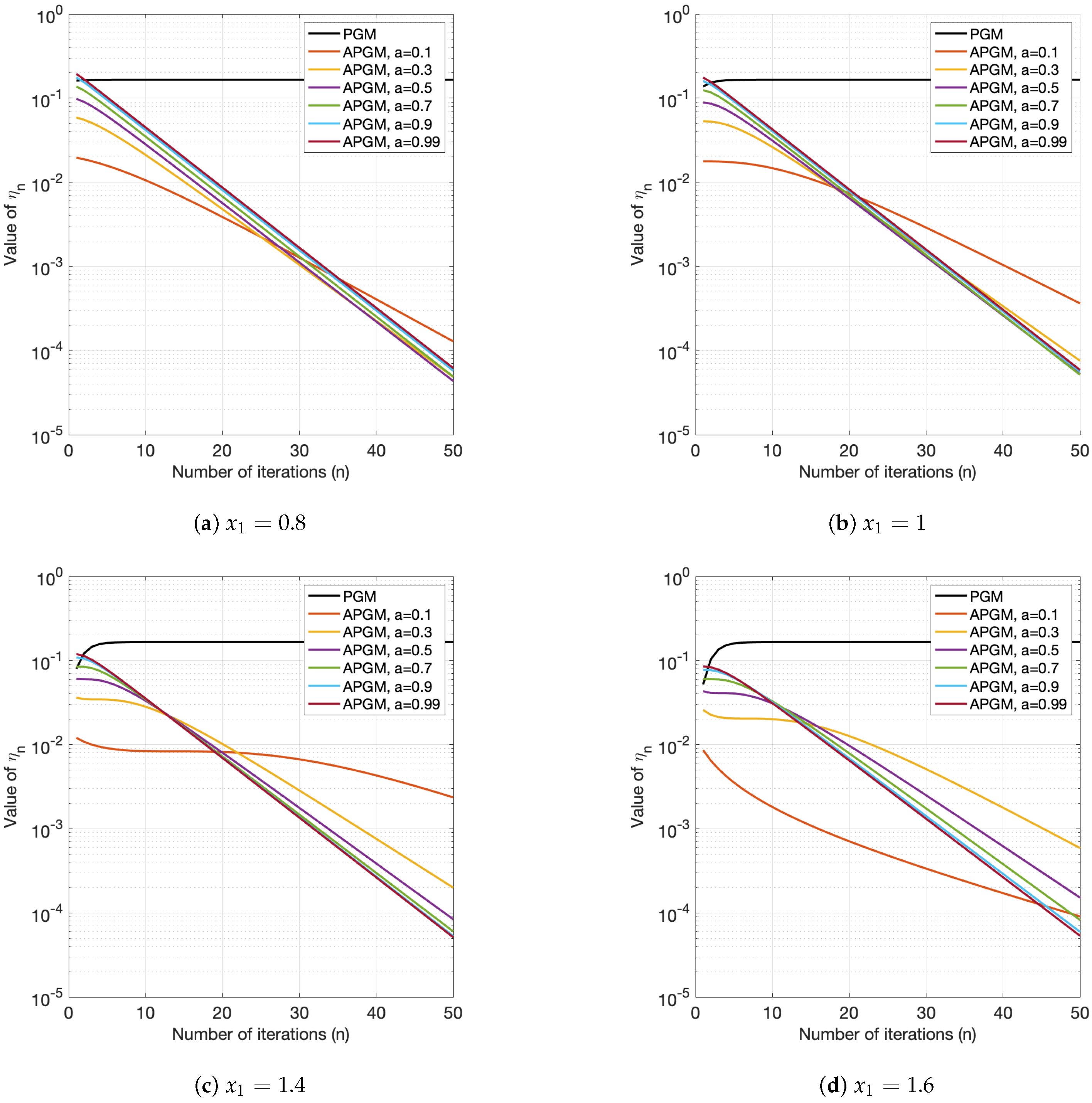
According to Figure 2, the values of η n tended to be nondecreasing throughout the considered iterations when performed by PGM, meanwhile the values of η n rapidly decreased for all values of the parameter a when performed by APGM. This numerical behavior of APGM demonstrated its theoretical perspective that was stated in Lemma 1.

4.2. Convex–Concave Fractional Programming with Linear Constraints

In this subsection, we present our considerations of the following convex–concave fractional programming with linear constraints:
minimize 0.5 x 2 10 0.5 x 2 subject to A x b x [ 0 , 1 ] 2
where
A : = 2 1 4 3 1 2 3 1 1 1 and b : = 2 4 2 4 2 .
By invoking the convex differentiable proximity function in which the weighted sum of the squared values of the constraints is minimal, we obtain
h ( x ) : = 0.5 i = 1 5 1 5 ( max { A ( i , : ) , x b ( i ) , 0 } ) 2 , x R 2 ,
so we can consider problem (16) as the following nonlinear convex–concave fractional programming:
min x [ 0 , 1 ] 2 0.5 x 2 + 0.5 i = 1 5 1 5 ( max { A ( i , : ) , x b ( i ) , 0 } ) 2 10 0.5 x 2 .
Note that function f ( x ) = 0.5 x 2 + 0.5 i = 1 5 1 5 ( max { A ( i , : ) , x b ( i ) , 0 } ) 2 is a convex differentiable with a gradient of the Lipschitz constant L f = 46 > 0 . Moreover, we observe that f ( x ) 0 for all x [ 0 , 1 ] 2 , which shows that assumption ( A f ) is satisfied. Furthermore, we observe that function g ( x ) = 10 0.5 x 2 is a concave differentiable with a gradient of the Lipschitz constant L g = 1 > 0 and we note that 0 < 9 g ( x ) 10 = : M for all x [ 0 , 1 ] 2 . This means that assumption ( A g ) is also satisfied. Thus, the considered problem fits into the framework of the fractional programming problem (1).
In the same fashion as the previous subsection, we now present the numerical experiment that illustrated the influence of APGM on various values of the initial point x 1 [ 0 , 1 ] 2 and various values of the parameter a ( 0 , 1 ) . We set the the lower bound as η ̲ = 10 10 . The behavior of the iterate x n , function value θ n and step-size η n for 500 iterations are presented in Figure 3, Figure 4 and Figure 5, respectively. It is worth mentioning that we did not include PGM ([30], Algorithm 6) in this experiment because this method was not appropriate for solving problem (17) as the computation of the proximal operator of the sum of the convex functions required the subproblem in each iteration (n) to be solved. Again, this demonstrates the advantages of our proposed APGM.
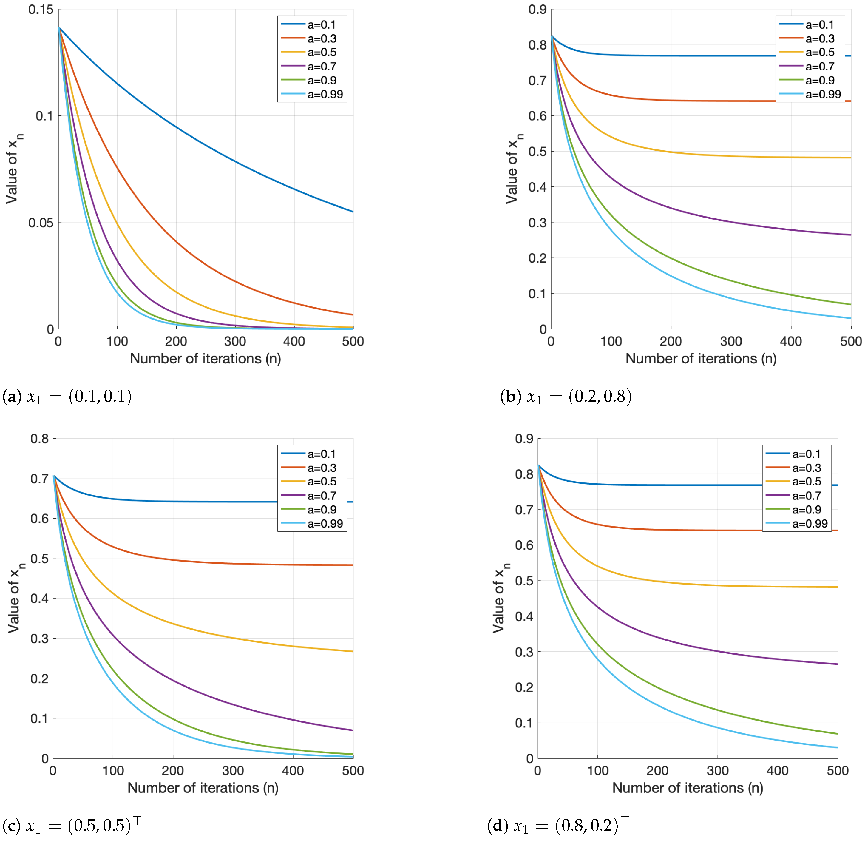
In Figure 3, it can be seen that for all different values of x 1 , APGM converged to their approximate solutions for all values of a. Moreover, it can also be seen that a = 0.99 yielded the fastest overall convergence for every value of x 1 . In particular, by using x 1 = ( 0.1 , 0.1 ) with a = 0.9 , APGM converged within only 200 iterations.
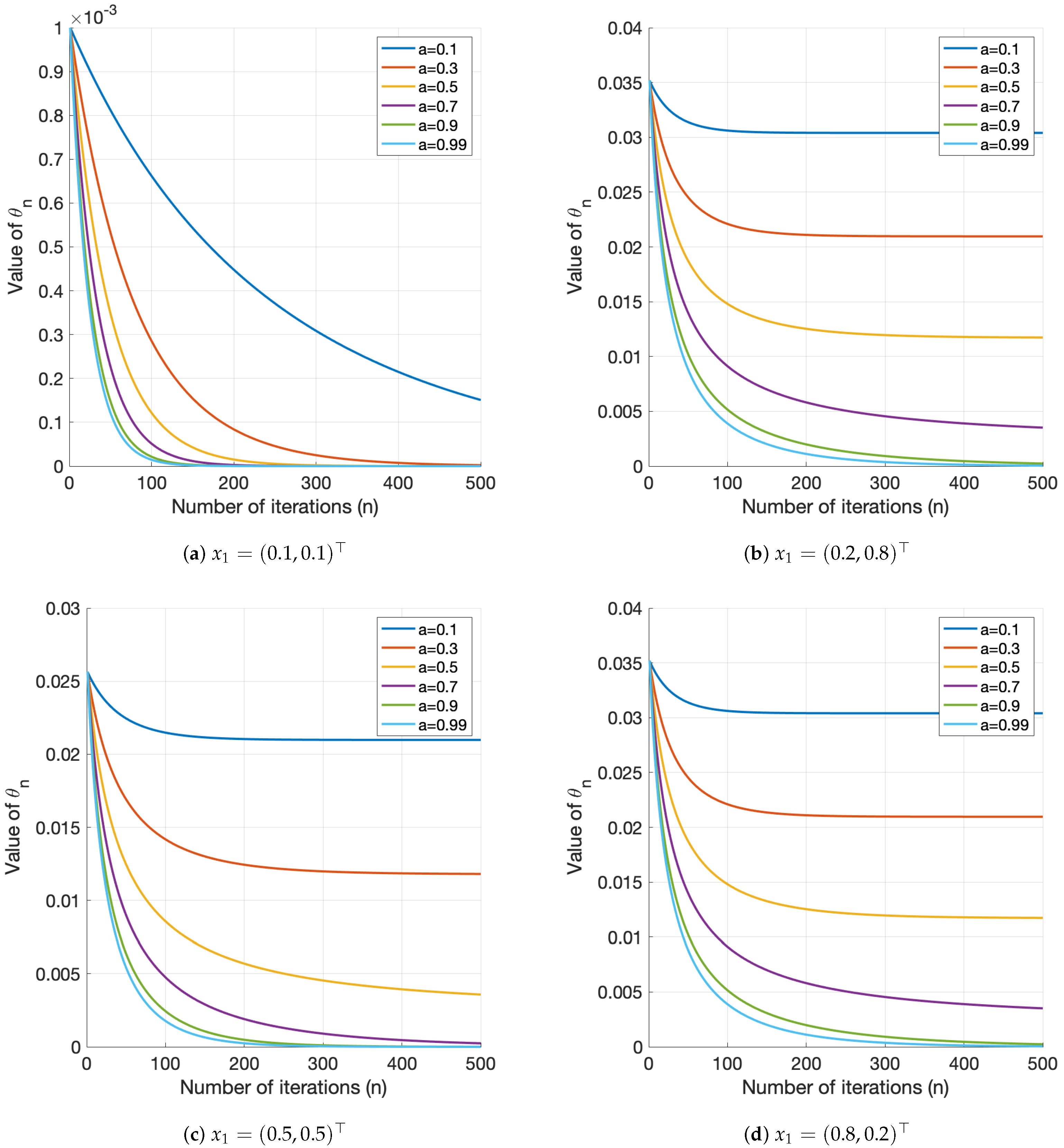
Figure 4 shows that the function values θ n of APGM for all values of x 1 and a tended to decrease to the optimal value. We noticed that the best overall performance was observed with a = 0.99 . Moreover, it can be seen that by using x 1 = ( 0.1 , 0.1 ) with a = 0.7 , 0.9 and 0.99 , the function values of APGM achieved their lowest values within only 200 iterations.
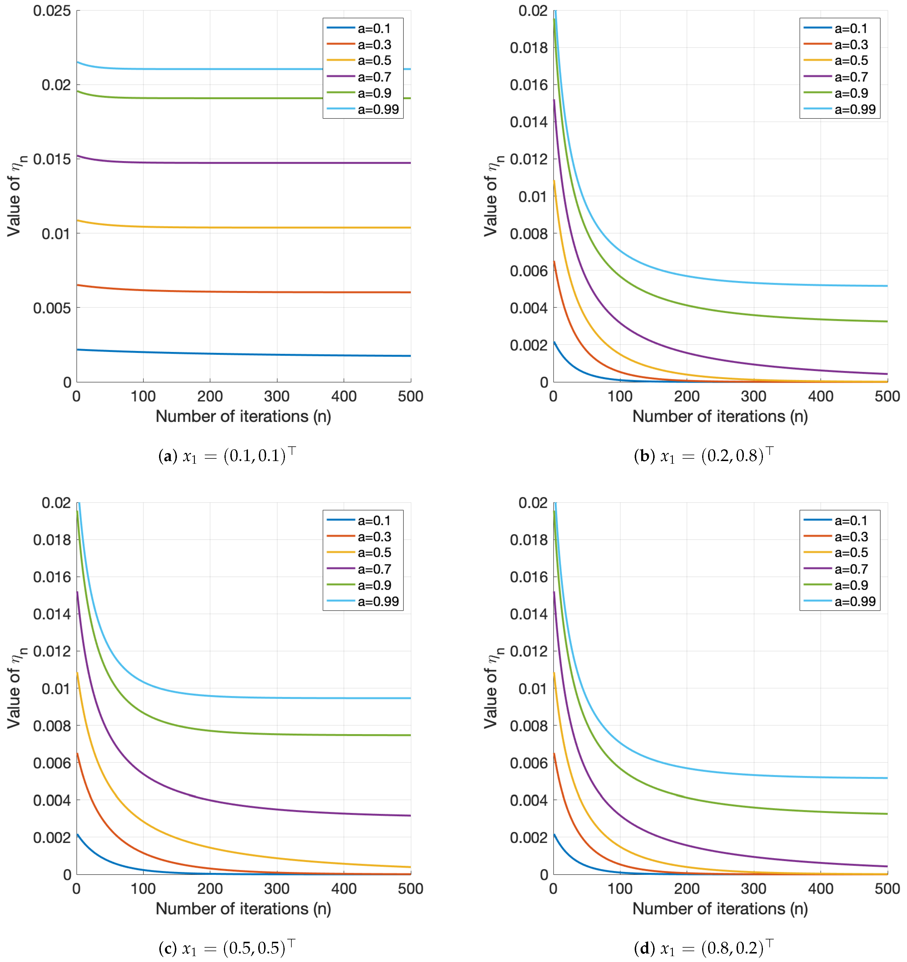
According to Figure 5, it can be seen that the values of η n appeared to be nonincreasing throughout the 500 iterations for all values of the parameter a when performed by APGM. This numerical behavior of APGM again demonstrates its theoretical perspective that was stated in Lemma 1. Moreover, we observed that the greatest value of η n was obtained with a = 0.99 , while the lowest value of η n occurred with a = 0.1 .

4.3. Quadratic Fractional Programming

In this subsection, we present our considerations of quadratic fractional programming in the following form ([31], Problem (23)):
min x [ 1 , 3 ] 5 x , A x + b , x + c d , x + r
where
A : = 5 1 2 0 2 1 6 1 3 0 2 1 3 0 1 0 3 0 5 0 2 0 1 0 4 , b : = 1 2 1 2 1 , d : = 1 0 1 0 1 ,
c : = 2 and r : = 20 . Note that function f ( x ) = x , A x + b , x + c is a convex differentiable with a gradient of the Lipschitz constant L f = 2 M > 0 . We observe that f ( x ) 34 > 0 for all x [ 1 , 3 ] 5 . This means that assumption ( A f ) is satisfied. Furthermore, function g ( x ) = d , x + r is an affine (i.e., concave) differentiable with a gradient of the Lipschitz constant L g = 0 . We note that 0 < 21 g ( x ) 23 = : M for all x [ 1 , 3 ] 5 , which means that assumption ( A g ) is also satisfied. Thus, the considered problem fits into the framework of the fractional programming problem (1).
In this numerical experiment, we explored the influence of APGM on the initial point x 1 : = ( 3 , 1.5 , 2 , 1.5 , 2 ) with different values of parameter a ( 0 , 1 ) . We set the lower bound as η ̲ = 10 10 . We compared the performance of APGM to that of the proximity gradient–sub-gradient algorithm (PGSA) for fractional programming, which was proposed in [8] (Algorithm 1). The behavior of the iterate x n and function value θ n are illustrated in Table 1.
It can be observed from Table 1 that both methods yielded almost the exact same results throughout the considered iterations. This was probably caused by the simplicity of the affine function g, which had a gradient of the Lipschitz constant L g = 0 . However, note that APGM and PGSA were studied in different settings, yet both methods achieved the same results.

5. Conclusions

In this paper, we presented our so-called adaptive projection gradient method for solving the nonlinear fractional optimization problem in which the numerator is smooth convex and the denominator is smooth concave. An interesting property that distinguished the proposed method from some existing methods was the nonincreasing property of the step-size sequence, which was stated in Lemma 1. We proved that the sequence of iterates that was generated by the proposed method converged to a solution for the considered problem. Finally, we also presented numerical experiments to illustrate the efficiency of the proposed method by applying APGM to solve three different types of the nonlinear fractional programming problem.

Author Contributions

Conceptualization, M.P., T.F. and N.N.; methodology, M.P., T.F. and N.N.; software, M.P., T.F. and N.N.; validation, M.P., T.F. and N.N.; convergence analysis, M.P. and N.N.; investigation, M.P., T.F. and N.N.; writing—original draft preparation, M.P., T.F. and N.N.; writing—review and editing, M.P., T.F. and N.N.; visualization, M.P., T.F. and N.N.; supervision, N.N.; project administration, N.N.; funding acquisition, N.N. All authors have read and agreed to the published version of the manuscript.

Funding

This research was supported by the Fundamental Fund of Khon Kaen University. This research received funding support from the National Science, Research and Innovation Fund or NSRF.

Informed Consent Statement

Not applicable.

Data Availability Statement

Not applicable.

Acknowledgments

The authors would like to thank the editors and anonymous referees for their comments and remarks, which improved the quality and presentation of the paper. Mootta Prangprakhon was partially supported by the Science Achievement Scholarship of Thailand (SAST) and the Faculty of Science at Khon Kaen University.

Conflicts of Interest

The authors declare no conflict of interest.

References

  1. Bradley, S.P.; Frey, S.C., Jr. Fractional programming with homogeneous functions. Oper. Res. 1974, 22, 350–357. [Google Scholar] [CrossRef]
  2. Charnes, A.; Cooper, W.W.; Rhodes, E. Measuring the efficiency of decision making units. Eur. J. Oper. Res. 1978, 2, 429–444. [Google Scholar] [CrossRef]
  3. Konno, H.; Inori, M. Bond portfolio optimization by bilinear fractional programming. J. Oper. Res. Soc. Jpn. 1989, 32, 143–158. [Google Scholar] [CrossRef]
  4. Pardalos, P.M.; Sandström, M.; Zopounidis, C. On the use of optimization models for portfolio selection: A review and some computational results. Comput. Econ. 1994, 7, 227–244. [Google Scholar] [CrossRef]
  5. Hyvärinen, A.; Oja, E. A fast fixed-point algorithm for independent component analysis. Neural Comput. 1997, 9, 1483–1492. [Google Scholar] [CrossRef]
  6. Hyvärinen, A.; Oja, E. Independent component analysis: Algorithms and applications. Neural Netw. 2000, 13, 411–430. [Google Scholar] [CrossRef] [Green Version]
  7. Li, Q.; Shen, L.; Zhang, N.; Zhou, J. A proximal algorithm with backtracked extrapolation for a class of structured fractional programming. Appl. Comput. Harmon. Anal. 2022, 56, 98–122. [Google Scholar] [CrossRef]
  8. Zhang, N.; Li, Q. First-order algorithms for a class of fractional optimization problems. SIAM J. Optim. 2022, 32, 100–129. [Google Scholar] [CrossRef]
  9. Shen, K.; Yu, W. Fractional programming for communication systems-part I: Power control and beamforming. IEEE Trans. Signal Process. 2018, 66, 2616–2630. [Google Scholar] [CrossRef] [Green Version]
  10. Zappone, A.; Björnson, E.; Sanguinetti, L.; Jorswieck, E. Globally optimal energy-efficient power control and receiver design in wireless networks. IEEE Trans. Signal Process. 2017, 65, 2844–2859. [Google Scholar] [CrossRef]
  11. Zappone, A.; Sanguinetti, L.; Debbah, M. Energy-delay efficient power control in wireless networks. IEEE Trans. Commun. 2017, 66, 418–431. [Google Scholar] [CrossRef] [Green Version]
  12. Chen, L.; He, S.; Zhang, S.Z. When all risk-adjusted performance measures are the same: In praise of the Sharpe ratio. Quant. Financ. 2011, 11, 1439–1447. [Google Scholar] [CrossRef]
  13. Archetti, C.; Desaulniers, G.; Speranza, M.G. Minimizing the logistic ratio in the inventory routing problem. EURO J. Transp. Logist. 2017, 6, 289–306. [Google Scholar] [CrossRef]
  14. Chen, F.; Huang, G.H.; Fan, Y.R.; Liao, R.F. A nonlinear fractional programming approach for environmental-economic power dispatch. Int. J. Electr. Power Energy Syst. 2016, 78, 463–469. [Google Scholar] [CrossRef]
  15. Rahimi, Y.; Wang, C.; Dong, H.; Lou, Y. A scale-invariant approach for sparse signal recovery. SIAM J. Sci. Comput. 2019, 41, 3649–3672. [Google Scholar] [CrossRef] [Green Version]
  16. Boţ, R.I.; Dao, M.N.; Li, G. Inertial proximal block coordinate method for a class of nonsmooth sum-of-ratios optimization problems. SIAM J. Optim. 2022; accepted. [Google Scholar]
  17. Stancu-Minasian, I.M. Fractional Programming: Theory, Methods, and Applications; Kluwer Academic Publishers: Boston, MA, USA, 1997. [Google Scholar]
  18. Stancu-Minasian, I.M. A ninth bibliography of fractional programming. Optimization 2019, 68, 2125–2169. [Google Scholar] [CrossRef]
  19. Dinkelbach, W. On nonlinear fractional programming. Manag. Sci. 1976, 13, 492–498. [Google Scholar] [CrossRef]
  20. Crouzeix, J.P.; Ferland, J.A.; Schaible, S. An algorithm for generalized fractional programs. J. Optim. Theory Appl. 1985, 47, 35–49. [Google Scholar] [CrossRef]
  21. Ibaraki, T. Parametric approaches to fractional programs. Math. Program. 1983, 26, 45–362. [Google Scholar] [CrossRef]
  22. Schaible, S. Fractional programming. II, on Dinkelbach’s algorithm. Manag. Sci. 1976, 22, 868–873. [Google Scholar] [CrossRef]
  23. Jagannathan, R. On some properties of programming problems in parametric form pertaining to fractional programming. Manag. Sci. 1966, 12, 609–615. [Google Scholar] [CrossRef]
  24. Bauschke, H.H.; Combettes, P.L. Convex Analysis and Monotone Operator Theory in Hilbert Spaces; CMS Books in Mathematics; Springer: New York, NY, USA, 2017. [Google Scholar]
  25. Boţ, R.I.; Dao, M.N.; Li, G. Extrapolated proximal sub-gradient algorithms for nonconvex and nonsmooth fractional programs. Math. Oper. Res. 2021. [Google Scholar] [CrossRef]
  26. Aragón Artacho, F.J.; Campoy, R.; Tam, M.K. Strengthened splitting methods for computing resolvents. Comput. Optim. Appl. 2021, 80, 549–585. [Google Scholar] [CrossRef]
  27. Cegielski, A. Iterative Methods for Fixed Point Problems in Hilbert Spaces; Lecture Notes in Mathematics 2057; Springer: Berlin, Germany, 2012. [Google Scholar]
  28. Polyak, B.T. Introduction to Optimization; Optimization Software: New York, NY, USA, 1987. [Google Scholar]
  29. Malitsky, Y.; Mishchenko, K. Adaptive gradient descent without descent. In Proceedings of the 37th International Conference on Machine Learning, Virtual, 13–18 July 2020; Volume 119 of Proceedings of Machine Learning Research. pp. 6702–6712. [Google Scholar]
  30. Boţ, R.I.; Csetnek, E.R. Proximal-gradient algorithms for fractional programming. Optimization 2017, 66, 1383–1396. [Google Scholar] [CrossRef] [PubMed] [Green Version]
  31. Boţ, R.I.; Csetnek, E.R.; Vuong, P.T. The forward-backward-forward method from continuous and discrete perspective for pseudo-monotone variational inequalities in Hilbert spaces. Eur. J. Oper. Res. 2020, 287, 49–60. [Google Scholar] [CrossRef]
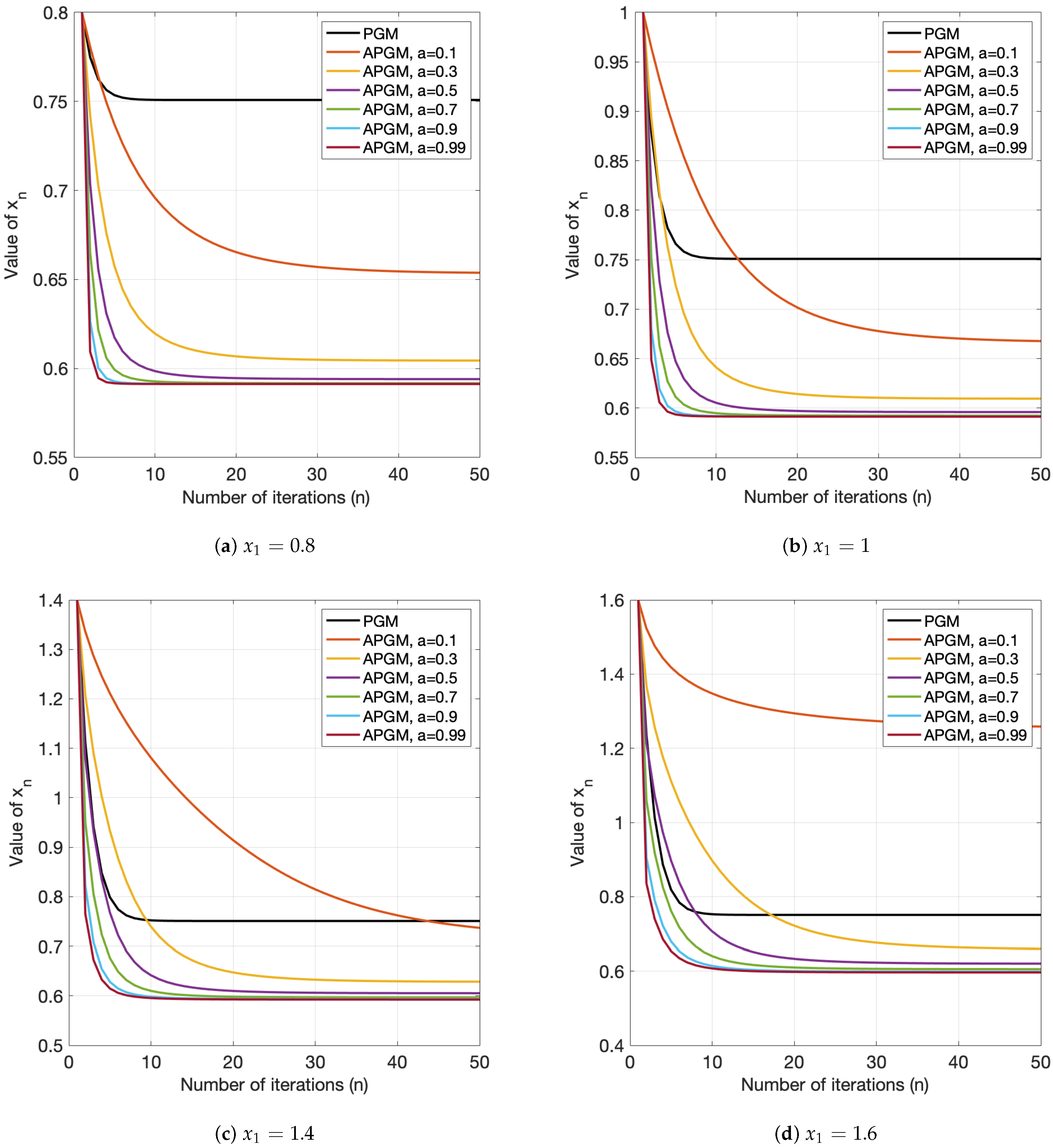
Figure 1. The behavior of the iterate x n for different values of the initial point x 1 when performed by PGM and APGM with various values for a.
Fractalfract 06 00566 g001
Figure 2. The behavior of the step size η n for different values of the initial point x 1 when performed by PGM and APGM with various values for a.
Fractalfract 06 00566 g002
Figure 3. The behavior of the iterate x n for different values of the initial point x 1 when performed by APGM with various values for a.
Fractalfract 06 00566 g003
Figure 4. The behavior of the function value θ n for different values of the initial point x 1 when performed by APGM with various values for a.
Fractalfract 06 00566 g004
Figure 5. The behavior of the step size η n for different values of the initial point x 1 when performed by APGM with various values for a.
Fractalfract 06 00566 g005
Table 1. The behavior of the iterate x n and function value θ n when performed by APGM and PGSA with various values for a.
anAPGMPGSA ([8], Algorithm 1)
x n θ n x n θ n
0.6 1 ( 3 , 1.5 , 2 , 1.5 , 2 ) 6.6630 ( 3 , 1.5 , 2 , 1.5 , 2 ) 6.6630
2 ( 1.7758 , 1 , 1 , 1 , 1.1365 ) 2.4070 ( 1.7758 , 1 , 1 , 1 , 1.1365 ) 2.4070
3 ( 1.0605 , 1 , 1 , 1 , 1 ) 1.6641 ( 1.0250 , 1 , 1 , 1 , 1 ) 1.6375
4 ( 1 , 1 , 1 , 1 , 1 ) 1.6190 ( 1 , 1 , 1 , 1 , 1 ) 1.6190
0.7 1 ( 3 , 1.5 , 2 , 1.5 , 2 ) 6.6630 ( 3 , 1.5 , 2 , 1.5 , 2 ) 6.6630
2 ( 1.5717 , 1 , 1 , 1 , 1 ) 2.1025 ( 1.5717 , 1 , 1 , 1 , 1 ) 2.1025
3 ( 1 , 1 , 1 , 1 , 1 ) 1.6190 ( 1 , 1 , 1 , 1 , 1 ) 1.6190
0.9 1 ( 3 , 1.5 , 2 , 1.5 , 2 ) 6.6630 ( 3 , 1.5 , 2 , 1.5 , 2 ) 6.6630
2 ( 1.1637 , 1 , 1 , 1 , 1 ) 1.7443 ( 1.1637 , 1 , 1 , 1 , 1 ) 1.7443
3 ( 1 , 1 , 1 , 1 , 1 ) 1.6190 ( 1 , 1 , 1 , 1 , 1 ) 1.6190
0.99 1 ( 3 , 1.5 , 2 , 1.5 , 2 ) 6.6630 ( 3 , 1.5 , 2 , 1.5 , 2 ) 6.6630
2 ( 1 , 1 , 1 , 1 , 1 ) 1.6190 ( 1 , 1 , 1 , 1 , 1 ) 1.6190
Publisher’s Note: MDPI stays neutral with regard to jurisdictional claims in published maps and institutional affiliations.