On Study of Modified Caputo–Fabrizio Omicron Type COVID-19 Fractional Model

Abstract

In this paper, we analyze the novel type of COVID-19 caused by the Omicron virus under a new operator of fractional order modified by Caputo–Fabrizio. The whole compartment is chosen in the sense of the said operator. For simplicity, the model is distributed into six agents along with the inclusion of the Omicron virus infection agent. The proposed fractional order model is checked for fixed points with the help of fixed point theory. The series solution is carried out by the technique of the Laplace Adomian decomposition technique. The compartments of the proposed problem are simulated for graphical presentation in view of the said technique. The numerical simulation results are established at different fractional orders along with the comparison of integer orders. This consideration will also show the behavior of the Omicron dynamics in human life and will be essential for its control and future prediction at various time durations. The sensitivity of different parameters is also checked graphically.

1. Introduction

From the outbreak of infection of COVID-19, different types of it due to several viruses have been discovered, like MERS-COVID, COVID-19, Omicron type COVID-19, etc. The Omicron type virus is a new infection of SARS-CoV-2 caused by the virus known as the Omicron virus. It is produced from the COVID-19 chain of SARS-CoV-2 (COVID-19), discovered in the month of November 2021 in the country of South Africa. After that, the said virus expansion occurs very quickly, and it is transmitted to many continents of the world. The cases of the Omicron disease are growing day by day. The disease of this virus is not more severe than the usual COVID-19 and its other types, but it infects very fast as compared with the other COVID-19 types. According to the reports of World Health Organization (WHO), it can affect the vaccinated population and those who do not have any proper symptoms of infection [1]. However, up to now, few common signs of this infection have been found, like coughing, congestion, watery nose, body aches, etc. Like the bans of COVID-19, this infection also faces bans on overcrowding, unmasking, traffic, and flight suspensions.

COVID-19 has been investigated by many researchers and biologists to control or reduce the infection and its further expansion in the human communities. They tried to find a treatment and a cure in the form of vaccination to vaccinate many people in order to minimize the number of infectious people and their future control. Still, with the duration of time and the emergency of the novel viruses of COVID-19, the world is facing such a type of pandemic in many countries and societies. Mathematical models touched on each and every infection in mathematical terms. Therefore, some mathematical models in natural and non-natural orders are considered to investigate the COVID-19 pandemic. For example, the first infection of COVID-19 in Wuhan, China in the sense of a very significant mathematical model, was studied in [2]. The optimal control techniques for the eradication or control of the infection in Pakistan, by proposing the real COVID-19 classes have been discussed in [3]. The COVID-19 disease is spread to healthy people very quickly, so the best and most effective framework to minimize the infection, is the self-isolation and quarantining technique, which is analyzed by a mathematical model established by scholars in [4]. The lockdown and its impacts on infection control have been investigated through a mathematical formulation technique in [5]. The researchers constructed an Susceptible-Exposed-Infectious-Recovered (SEIR) model by using the realistic data approach from France and Italy and established the disease control techniques [6]. Various reports related to COVID-19 cases and their formulation in Nigeria, by comparison, have been given in [7]. A global analysis on COVID-19 to study the self-isolation, quarantined, and environmental vital wights has been pointed out in [8]. A comprehensive discussion on COVID-19 in the framework of fractional environment is carried out in [9]. The discussion of the COVID-19 disease modeling the realistic cases in Saudi Arabia has been established in [10].

Mathematical formulations provide a comprehensive tool for the analysis of different dynamics of social, physical, and biological problems. Most linear phenomena are generally idealistic and not realistic, as several real-world phenomena are non-linear. As a result, non-linear mathematical models for real-world problems are superior to linear models. So far, a number of attempts have been made by different scientists to mathematically formulate the dynamics and control of this novel Omicron type virus COVID-19 infection. The Omicron infection of November 2021, which occurred in African and European countries, has been investigated in detail by Altaf et al. [11]. By the application of the controlling theory of optimality, they minimize the said infection [12]. Vaccination and curing have also reduced the transmission of the Omicron virus COVID-19 [13].

In the article of Altaf et al. [14], the six compartmental model subject to the initial conditions along with the inclusion of the Omicron virus agent is considered as follows:

$$\begin{array}{c}\hfill \begin{array}{cc}& \frac{d}{dt}\left(\mathbb{S}\left(\tau \right)\right)=\lambda -\frac{\alpha ({\mathbb{I}}_{\alpha }\left(\tau \right)+\kappa {\mathbb{I}}_s\left(\tau \right)+u{\mathbb{I}}_O\left(\tau \right)\mathbb{S}\left(\tau \right))}{N}-\nu \mathbb{S}\left(\tau \right),\hfill \\ & \frac{d}{dt}\left(\mathbb{E}\left(\tau \right)\right)=\frac{\alpha ({\mathbb{I}}_{\alpha }\left(\tau \right)+\kappa {\mathbb{I}}_s\left(\tau \right)+u{\mathbb{I}}_O\left(\tau \right)\mathbb{S}\left(\tau \right))}{N}-(\tau +\nu )\mathbb{E}\left(\tau \right),\hfill \\ & \frac{d}{dt}\left({\mathbb{I}}_{\beta }\left(\tau \right)\right)=\tau \Psi \mathbb{E}\left(\tau \right)-({\Delta }_1+\nu ){\mathbb{I}}_{\beta }\left(\tau \right),\hfill \\ & \frac{d}{dt}\left({\mathbb{I}}_s\left(\tau \right)\right)=(1-\Psi -\varphi )\tau \mathbb{E}\left(\tau \right)-({\Delta }_2+\nu +{\delta }_1){\mathbb{I}}_s\left(\tau \right),\hfill \\ & \frac{d}{dt}\left({\mathbb{I}}_O\left(\tau \right)\right)=\varphi \tau \mathbb{E}\left(\tau \right)-({\Delta }_3+\nu ){\mathbb{I}}_O\left(\tau \right),\hfill \\ & \frac{d}{dt}\left(\mathbb{R}\left(\tau \right)\right)={\Delta }_1{\mathbb{I}}_{\beta }\left(\tau \right)+{\Delta }_2{\mathbb{I}}_s\left(\tau \right)+{\Delta }_3{\mathbb{I}}_O\left(\tau \right)-\nu \mathbb{R}\left(\tau \right),\hfill \\ & \mathbb{S}\left(0\right)={\mathbb{S}}_0\ge 0,\mathbb{E}\left(0\right)={\mathbb{E}}_0\ge 0,{\mathbb{I}}_{\beta }\left(0\right)={\mathbb{I}}_{\left(\beta \right)0}\ge 0,{\mathbb{I}}_s\left(0\right)={\mathbb{I}}_{\left(s\right)0}\ge 0,\hfill \\ & {\mathbb{I}}_O\left(0\right)={\mathbb{I}}_{\left(O\right)0}\ge 0,\mathbb{R}\left(0\right)={\mathbb{R}}_0\ge 0.\hfill \end{array}\end{array}$$

(1)

The compartments and parameters of the above model are defined in Table 1.

Table 1. Description of the parameter of (1).

Notation	Description of the Parameter
$\mathbb{S}\left(t\right)$	Susceptible or healthy class
$\mathbb{E}\left(t\right)$	Exposed class
${\mathbb{I}}_{\alpha }\left(t\right)$	Asymptomatic individuals having no symptoms
${\mathbb{I}}_s\left(t\right)$	Symptomatic individuals having symptoms of COVID-19
${\mathbb{I}}_O\left(t\right)$	Infection with Omicron virus
$\mathbb{R}\left(t\right)$	Recovered class from all type of infections
$\lambda$	Rate of birth to susceptible population
$\alpha$	Rate of infection of susceptible peoples from asymptomatic infection
$\kappa$	Probability of infectiousness of symptomatic class
u	Naturally death rate
$\nu$	Probability of infection through omicron variant
$\tau$	Infection incubation period
$\Psi$	Proportion contribution of infection to asymptomatic population
$\varphi$	Proportion contribution of infection to Omicron variant population
${\Delta }_1$	Rate of recovery of asymptomatic class
${\Delta }_2$	Rate of recovery of symptomatic class
${\Delta }_3$	Rate of recovery of Omicron variant infection
$d_1$	Rate of death of symptomatic class

For the analysis of fractional problems, different operators, including fractal derivative, non-integer order derivatives with kernels of singularity and non-singularity, fractional–fractal operator, and some other derivative operators, have been introduced in [15,16,17,18,19,20]. The inclusion of fractional derivative terms in the form of deterministic equations has more realistic achievements. The analysis of inside properties is found in many infectious disease models, the flow of heat, fluid flow, and many complex advection problems [19,21,22,23]. Several authors have used different techniques of fractional calculus by applying different operators and studying several types of disease models such as the coronavirus model, co-infection model, typhoid disease model, etc. [24,25,26,27]. In fractional calculus, the exponential and Mittag–Leffler mappings are not able to find the inside dynamics. Therefore, to solve such problems, one of the advanced approaches to fractional differentiation and integration has been introduced by many researchers. They introduced the classical and global derivatives along with some applicable examples [28,29,30,31]. We will investigate the said problem for qualitative analysis and numerical analysis in the sense of Modified Caputo–Fabrizio (MCF) fractional derivative. In the sense of a non-singular kernel, (1) can be written in Modified Caputo derivative format as follows:

$$\begin{array}{c}\hfill \begin{array}{cc}& {}^{CF}{\mathbf{D}}^{\wp }\left(\mathbb{S}\left(\tau \right)\right)=\lambda -\frac{\alpha ({\mathbb{I}}_{\alpha }\left(\tau \right)+\kappa {\mathbb{I}}_s\left(\tau \right)+u{\mathbb{I}}_O\left(\tau \right)\mathbb{S}\left(\tau \right))}{N}-\nu \mathbb{S}\left(\tau \right),\hfill \\ & {}^{CF}{\mathbf{D}}^{\wp }\left(\mathbb{E}\left(\tau \right)\right)=\frac{\alpha ({\mathbb{I}}_{\alpha }\left(\tau \right)+\kappa {\mathbb{I}}_s\left(\tau \right)+u{\mathbb{I}}_O\left(\tau \right)\mathbb{S}\left(\tau \right))}{N}-(\tau +\nu )\mathbb{E}\left(\tau \right),\hfill \\ & {}^{CF}{\mathbf{D}}^{\wp }\left({\mathbb{I}}_{\beta }\left(\tau \right)\right)=\tau \Psi \mathbb{E}\left(\tau \right)-({\Delta }_1+\nu ){\mathbb{I}}_{\beta }\left(\tau \right),\hfill \\ & {}^{CF}{\mathbf{D}}^{\wp }\left({\mathbb{I}}_s\left(\tau \right)\right)=(1-\Psi -\varphi )\tau \mathbb{E}\left(\tau \right)-({\Delta }_2+\nu +{\delta }_1){\mathbb{I}}_s\left(\tau \right),\hfill \\ & {}^{CF}{\mathbf{D}}^{\wp }\left({\mathbb{I}}_O\left(\tau \right)\right)=\varphi \tau \mathbb{E}\left(\tau \right)-({\Delta }_3+\nu ){\mathbb{I}}_O\left(\tau \right),\hfill \\ & {}^{CF}{\mathbf{D}}^{\wp }\left(\mathbb{R}\left(\tau \right)\right)={\Delta }_1{\mathbb{I}}_{\beta }\left(\tau \right)+{\Delta }_2{\mathbb{I}}_s\left(\tau \right)+{\Delta }_3{\mathbb{I}}_O\left(\tau \right)-\nu \mathbb{R}\left(\tau \right),\hfill \\ & \mathbb{S}\left(0\right)={\mathbb{S}}_0\ge 0,\mathbb{E}\left(0\right)={\mathbb{E}}_0\ge 0,{\mathbb{I}}_{\beta }\left(0\right)={\mathbb{I}}_{\left(\beta \right)0}\ge 0,{\mathbb{I}}_s\left(0\right)={\mathbb{I}}_{\left(s\right)0}\ge 0,\hfill \\ & {\mathbb{I}}_O\left(0\right)={\mathbb{I}}_{\left(O\right)0}\ge 0,\mathbb{R}\left(0\right)={\mathbb{R}}_0\ge 0.\hfill \end{array}\end{array}$$

(2)

As far as the novelty is concerned, we converted the integer order model to a fractional MCF operator. As MCF operators are fractionalized derivative orders, therefore, they have an extra degree of freedom and choices. We have checked the dynamics of different fractional orders lying between 0 and 1, and compared them with the integer order. On small fractional orders, stability is achieved quickly, and vice versa. The fractional model is investigated for the existence and uniqueness of solution in the sense of the MCF operator. The approximate or series solution is obtained by the well-known Laplace Adomian decomposition method under the mentioned operator. All the quantities in the proposed problem are converging to their equilibrium points.

This paper is organized as follows: Section 2 is related to basic definitions taken from the literature of fractional calculus. In Section 3, the existence results and uniqueness of the solution is presented for the considered model. A series solution is obtained for the system with the help of Laplace Adomian decomposition method in Section 4. In Section 5, we presented the obtained solution graphically and explained the dynamical behavior for each compartment. Finally, we conclude our work in Section 6.

2. Preliminaries

Here, we include some definitions regarding this article.

Definition 1.

[32] Let a function be$\mathrm{\Phi }\in {\mathrm{H}}^1[0,T]$and$0<T$, $\wp \in (0,1),$then the Caputo–Fabrizio fractional derivative (CFFD) is defined as

$${}^{CF}{\mathbf{D}}^{\wp }(\Phi \left(\tau \right))=\frac{\mathbf{M}(\wp )}{(1-\wp )}{\int }_0^t{\Phi }^{\prime }\left(\tau \right)exp\left[-\wp \frac{t-\zeta }{1-\wp }\right]d\zeta ,$$

where $\mathbf{M}(\wp )$ is $\mathbf{M}(\wp )=\frac{2}{2-\wp },0<\wp \le 1$. Furthermore, $\mathbf{M}\left(0\right)=1.$ If Φ∉ in ${\mathrm{H}}^1(0,T)$, so the CF operator is

$${}^{CF}{\mathbf{D}}^{\wp }(\Phi \left(\tau \right))=\frac{\mathbf{M}(\wp )}{(1-\wp )}{\int }_0^t(\Phi \left(\tau \right)-\Phi \left(\zeta \right))exp\left[-\wp \frac{t-\zeta }{1-\wp }\right]d\zeta .$$

Definition 2.

[33] Let$\Phi \left(\tau \right):[a,\infty )\to R$be a smooth function with$a<0$ and $t>0$, and then the modified CF operator is given as

$$\begin{array}{c}\hfill {}^{MCF}{\mathbf{D}}^{\wp }(\Phi \left(\tau \right))=\frac{1}{1-\wp }{\int }_0^t\left({\psi }_0^{\prime }\left(\zeta \right)\beta (t-\zeta )+{\Phi }^{\prime }\left(\zeta \right)exp\left(-\frac{\wp }{1-\wp }(t-\zeta )\right)\right)d\zeta ,\end{array}$$

(3)

where

$$\begin{array}{c}\hfill {\psi }_0^{\prime }\left(\zeta \right)={\int }_a^0{\Phi }^{\prime }\left(\zeta \right)exp\left(-\frac{\wp }{1-\wp }(t-\zeta )\right)d\zeta .\end{array}$$

(4)

Definition 3.

[32] Suppose $\wp \in ]0,1[,$ then CF integral having order ℘ of Φ is

$${}^{CF}{I}^{\wp }[\Phi \left(\tau \right)]=G\Phi \left(\tau \right)+\overline{G}{\int }_0^t\Phi \left(\zeta \right)d\zeta ,\tau \ge 0,$$

when $\wp =1$, one can obtain classical integral of Φ, where

$$G=\frac{(1-\wp )}{\mathbf{M}(\wp )},\overline{G}=\frac{\wp }{\mathbf{M}(\wp )}.$$

Definition 4.

The Laplace transform of CF operator is

$$\mathcal{L}\left\{{}^{Modified-CF}{D}_x^{\wp }\Phi (x,\tau )\right\}=\frac{a(2-\wp )}{2(s+(1-s)\wp )}\left[{\zeta }^{n+1}\overline{\Phi }(s,\tau )-\sum _{k=0}^n{s}^{n-k}\left\{\frac{{\partial }^k\Phi (0,t)}{\partial x^k}\right\}\right],$$

where, $n=[\wp ]+1$

3. Qualitative Analysis

This section deals with the existence and uniqueness of solution of the considered model (2). To do this, we need the following theorem from fixed point theory.

Existence and Uniqueness Solution of Model (2)

To prove the results, we give the following notions and lemma.

Consider $\Phi =[0,1]$ and $\mathcal{C}(\Phi )$ represents the space containing continuous functions on $\Phi$. Consider set $B=\mathcal{W}\left(\tau \right)/\mathcal{W}\left(\tau \right)\in \mathcal{C}(\Phi )$ with ${\left|\right|\mathcal{W}\left(\tau \right)\left|\right|}_b\le {max}_{t\in \Phi }\left|\mathcal{W}\left(\tau \right)\right|$ represents Banach space. For simplicity, consider $\mathcal{W}\left(\tau \right)=\Phi (\tau ,\Omega \left(\tau \right)),\nu \left(\tau \right)={\Phi }_1(t,{\Omega }_1\left(\tau \right))$ and $\mathcal{W}\left(0\right)=\Omega \left(0\right)={\mathcal{W}}_0$ and $\mathcal{V}\left(0\right)={\Omega }_1\left(0\right)={\mathcal{V}}_0$. The model (2) in integral form is

$$\mathcal{W}\left(\tau \right)={\mathcal{W}}_0+\frac{2(1-\wp )}{(2-\wp )\mathbf{M}(\wp )}(\Phi (\tau ,\Omega \left(\tau \right)))+\frac{(2\wp )}{(2-\wp )\mathbf{M}(\wp )}{\int }_0^t\Phi (\zeta ,\Omega \left(\zeta \right))d\zeta .$$

Let us suppose an operator $\mathcal{T}:\mathbb{B}\to \mathbb{B}$ defined as

$$\mathcal{T}\mathcal{W}\left(\tau \right)={\mathcal{W}}_0+\frac{2(1-\wp )}{(2-\wp )\mathbf{M}(\wp )}(\Phi (\tau ,\Omega \left(\tau \right))+\frac{(2\wp )}{(2-\wp )\mathbf{M}(\wp )}{\int }_0^t\Phi (\zeta ,\Omega \left(\zeta \right))d\zeta ,$$

and then operator $\mathcal{T}$ has same fixed-point (FP) as (2).

Theorem 1.

Suppose a continuous function to be$f:\Phi \times \mathcal{R}\to \mathcal{R}$. Also, consider in the following at least one is satisfied.

$\left({\mathcal{H}}_1\right)$

Let the function$g\left(\tau \right)\in L[0,1]$exists which is non-negative, such that

$$|\Phi (\tau ,x)|\le h\left(\tau \right)+c_0{\left|x\right|}^{\zeta },here,c_0\ge 0,0<\zeta <1.$$

$\left({\mathcal{H}}_2\right)$

The function Φ satisfies$|\Phi (\tau ,x)|\le c_0{\left|x\right|}^{\zeta }$, where$c_0>0$,$\zeta >1$. Then model (2) has a solution.

Proof. 

By using the Schauder FP theorem to prove the results, consider, $\left({\mathcal{H}}_1\right)$ is holds. Let us consider $\mathbb{G}=\left\{\mathcal{W}\left(\tau \right)\right|\mathcal{W}\left(\tau \right)\in \mathbb{B},\parallel \mathcal{W}{\parallel }_{\mathbb{B}}\le k,t\in \Phi \}$, where $k\ge max{\left(2A{c}_0\right)}^{\left(\frac{1}{1-\zeta }\right)},2l$ and $l={max}_{y\in \Phi }\left({\mathcal{W}}_0+\frac{4(1-\wp )}{(2-\wp )\mathbf{M}(\wp )g\left(\tau \right)}+\frac{(2\wp )}{(2-\wp )\mathbf{M}(\wp )}{\int }_0^t\left|g\left(\zeta \right)\right|d\zeta \right)$. Obviously, $\mathbb{G}$ is a ball in $\mathbb{B}$. Furthermore, we prove that $\mathcal{T}:\mathbb{G}\to \mathbb{G}$. For all $u\in \mathbb{G}$, we have

$$\begin{array}{cc}& \left|\mathcal{T}\mathcal{W}\left(\tau \right)\right|=|{\mathcal{W}}_0+\frac{2(1-\wp )}{(2-\wp )\mathbf{M}(\wp )}(\Phi (\tau ,\Omega \left(\tau \right)))+\frac{(2\wp )}{(2-\wp )\mathbf{M}(\wp )}{\int }_0^t\Phi (\zeta ,\Omega \left(\zeta \right))d\zeta |\hfill \\ & \le {\mathcal{W}}_0+\frac{2(1-\wp )}{(2-\wp )\mathbf{M}(\wp )}|\Phi (\tau ,\Omega \left(\tau \right))|+\frac{2(1-\wp )}{(2-\wp )\mathbf{M}(\wp )}+\frac{(2\wp )}{(2-\wp )\mathbf{M}(\wp )}{\int }_0^t\Phi (\zeta ,\Omega \left(\zeta \right))d\zeta \hfill \\ & \le {\mathcal{W}}_0+\frac{4(1-\wp )}{(2-\wp )\mathbf{M}(\wp )}\left(g\left(\tau \right)+c_0{k}^{\zeta }\right)+\frac{(2\wp )}{(2-\wp )\mathbf{M}(\wp )}{\int }_0^t(g\left(\zeta \right)+c_0{k}^{\zeta })d\zeta \hfill \\ & \le {\mathcal{W}}_0+\frac{4(1-\wp )}{(2-\wp )\mathbf{M}(\wp )}\left(g\left(\tau \right)+c_0{k}^{\zeta }\right)+\frac{2\wp c_0{k}^{\zeta }t}{(2-\wp )\mathbf{M}(\wp )}+\frac{(2\wp )}{(2-\wp )\mathbf{M}(\wp )}{\int }_0^t(g\left(\zeta \right)d\zeta \hfill \\ & \le {\mathcal{W}}_0+\frac{4(1-\wp )}{(2-\wp )\mathbf{M}(\wp )}g\left(\tau \right)+\frac{(2\wp )}{(2-\wp )\mathbf{M}(\wp )}{\int }_0^t(g\left(\zeta \right)d\zeta +\left(\frac{4(1-\wp )}{(2-\wp )\mathbf{M}(\wp )}+\frac{2\wp t}{(2-\wp )\mathbf{M}(\wp )}\right)c_0{k}^{\zeta }\hfill \\ & \le {\mathcal{W}}_0+\frac{4(1-\wp )}{(2-\wp )\mathbf{M}(\wp )}g\left(\tau \right)+\frac{(2\wp )}{(2-\wp )\mathbf{M}(\wp )}{\int }_0^{t}g\left(\zeta \right)d\zeta +\left(\frac{4(1-\wp )}{(2-\wp )\mathbf{M}(\wp )}+\frac{2c_0{k}^{\zeta }}{M(\wp )}\right).\hfill \end{array}$$

Therefore,

$$\begin{array}{cc}\hfill & {\left|\right|\mathcal{T}\mathcal{W}\left(\tau \right)\left|\right|}_B=\underset{t\in \Phi }{max}\left|\mathcal{T}\mathcal{W}\left(\tau \right)\right|\hfill \\ & \le l+\frac{2c_0{k}^{\zeta }}{\mathbf{M}(\wp )}=l+A{c}_0{k}^{\zeta }\le \frac{k}{2}+\frac{k}{2}=k.\hfill \end{array}$$

Thus, the operator $T\mathcal{W}\left(\tau \right)$ is continuous on $\Phi$.

Next, suppose that the assumption $\left({\mathcal{H}}_2\right)$ is also satisfied by selecting $0\le k\le \left(\frac{1}{A{c}_0}\right)(\frac{1}{\zeta -1})$. Take into account the same procedure as used above, we obtain

$${\parallel \mathcal{T}\mathcal{W}\parallel }_{\mathbb{B}}\le A{c}_0{k}^{\zeta }\le k.$$

Finally, we obtain $\mathcal{T}:\mathbb{G}\to \mathbb{G}$ that the operator $\mathcal{T}$ is continuous because of the continuity of $\Phi$.

Next, we prove that the operator T is continuous completely. Let $R={max}_{t\in \Phi }|\Phi (\tau ,\Omega \left(\tau \right))|$, for any $\Phi \in \mathbb{G}$. Let $\left({\tau }_1\right),\left({\tau }_2\right)\in \Phi$ such that $\left({\tau }_1\right)<\left({\tau }_2\right)$.

Also, let ${\Psi }_1=\frac{2(1-\wp )}{(2-\wp )\mathbf{M}(\wp )}$ and ${\Psi }_2=\frac{2\wp }{(2-\wp )\mathbf{M}(\wp )}$, and we get

$$\begin{array}{cc}\hfill & |T\Phi \left({\tau }_2\right)-T\Phi \left({\tau }_1\right)|=|{\mathcal{W}}_0+{\Psi }_1\left[\mathcal{W}({\tau }_2,\Phi \left({\tau }_2\right))\right]+{\Psi }_2{\int }_0^{\left({\tau }_2\right)}f(\zeta ,u\left(\zeta \right))d\zeta \hfill \\ & -{\mathcal{W}}_0-{\Psi }_1\left[\mathcal{W}({\tau }_1,\Phi \left({\tau }_1\right))\right]+{\Psi }_2{\int }_0^{\left({\tau }_2\right)}\mathcal{W}(\zeta ,u\left(\zeta \right))d\zeta |\hfill \\ & =|{\Psi }_1[\mathcal{W}({\tau }_2,\Phi \left({\tau }_2\right))-\mathcal{W}({\tau }_1,\Phi \left({\tau }_1\right))]+{\Psi }_2{\int }_{\left({\tau }_1\right)}^{\left({\tau }_2\right)}\Phi (\zeta ,u\left(\zeta \right))d\zeta |\hfill \\ & \le {\Psi }_1\left|\mathcal{W}({\tau }_2,\Phi \left({\tau }_2\right))\right|+{\Psi }_1\left|\mathcal{W}({\tau }_1,\Phi \left({\tau }_1\right))\right|+{\Psi }_2{\int }_{\left({\tau }_1\right)}^{\left({\tau }_2\right)}\left|\mathcal{W}(\zeta ,u\left(\zeta \right))\right|d\zeta \hfill \\ & \le 2R{\Psi }_1+R{\Psi }_2{\int }_{\left({\tau }_1\right)}^{\left({\tau }_2\right)}d\zeta =R(2{\Psi }_1+{\Psi }_2(\left({\tau }_2\right)-\left({\tau }_1\right))).\hfill \end{array}$$

According to uniform continuity of the function $({\tau }_2-{\tau }_1)$ on interval $\Phi$, we prove that $\mathcal{T}\mathbb{G}$ is an equicontinuous set. From the above theorems, we observe that this function is uniformly bounded as $\mathcal{T}\mathbb{G}\subseteq \mathbb{G}$; therefore $\mathcal{T}$ is completely continuous. So by using the Schauder FP theorem, ∃ a solution of Equation (2) in the set $\mathbb{G}$. □

Corollary 1.

Suppose a bounded continuous function be$\mathcal{W}$on$\Phi \times \mathrm{R}$, and then Equation (2) has a solution.

Proof. 

As we know that $\mathcal{W}$ is continuous as well as bounded on $\Phi \times \mathrm{R}$, ∃$L>0$, satisfying $\left|\mathcal{W}\right|<L$. Consider $h\left(\tau \right)=L,c_0=0$ in $\left({\mathcal{H}}_1\right)$ of 1, then the model (2) has a solution.

Next we use the Banach contraction principle to establish uniqueness results for solutions to (2). □

Theorem 2.

Suppose that$\mathcal{W}:let\Phi \times \mathrm{R}\to \mathrm{R}$be a continuous function, which also satisfied the following conditions.

$\left({\mathcal{H}}_3\right)$

Consider function$h\left(\tau \right)\in L[0,1]$exists which is non-negative, such that

$$\left|\mathcal{W}\right(\tau \left)\right|\le h|\Phi (\tau ,\Omega \left(\tau \right)\left)\right|,t\in [0,1].$$

In addition, function$\mathcal{W}$ satisfies $\mathcal{W}\left(0\right)=0$

$\left(H_{\mathcal{H}}\right)$

Consider that$\zeta ={max}_{t\in \Phi }|\frac{2(1-\wp )}{(2-\wp )\mathbf{M}(\wp )}h\left(\tau \right)+\frac{(2\wp )}{(2-\wp )\mathbf{M}(\wp )}{\int }_0^t\left|h\left(\zeta \right)\right|d\zeta |<1$, Then model (2) has a unique solution.

Proof. 

We represent the operator $\mathcal{T}$ as

$$\begin{array}{cc}\hfill & \mathcal{T}\mathcal{W}\left(\tau \right)={\mathcal{W}}_0+\frac{2(1-\wp )}{(2-\wp )\mathbf{M}(\wp )}\Phi (\tau ,\Omega \left(\tau \right))+\frac{(2\wp )}{(2-\wp )\mathbf{M}(\wp )}{\int }_0^t|\Phi (\zeta ,u\left(\zeta \right))|d\zeta .\hfill \end{array}$$

For $\mathcal{W}\left(\tau \right)\in \mathbb{B}$, we get

$$\begin{array}{cc}\hfill & \left|\mathcal{T}\mathcal{W}\left(\tau \right)\right|=|{\mathcal{W}}_0+\frac{2(1-\wp )}{(2-\wp )\mathbf{M}(\wp )}\Phi (\tau ,\Omega \left(\tau \right))+\frac{(2\wp )}{(2-\wp )\mathbf{M}(\wp )}{\int }_0^t|\Phi (\zeta ,u\left(\zeta \right))|d\zeta ,\hfill \\ & \le |\Phi |+|\frac{2(1-\wp )}{(2-\wp )\mathbf{M}(\wp )}\Phi (\tau ,\Omega \left(\tau \right))|+\left|\frac{(2\wp )}{(2-\wp )\mathbf{M}(\wp )}{\int }_0^t\right|\Phi (\zeta ,u\left(\zeta \right))|d\zeta \hfill \\ & \le \left|{\mathcal{W}}_0\right|+\frac{2(1-\wp )}{(2-\wp )\mathbf{M}(\wp )}h\left(\tau \right)\left|\mathcal{W}\left(\tau \right)\right|+\frac{(2\wp )}{(2-\wp )\mathbf{M}(\wp )}{\int }_0^{t}h\left(\zeta \right)|u\left(\zeta \right)d\zeta \hfill \\ & \le \left|{\mathcal{W}}_0\right|+\left(\frac{2(1-\wp )}{(2-\wp )\mathbf{M}(\wp )}h\left(\tau \right)+\frac{(2\wp )}{(2-\wp )\mathbf{M}(\wp )}{\int }_0^{t}h\left(\zeta \right)d\zeta \right)\left|\right|u\left|\right|,\hfill \end{array}$$

and we have

$$\begin{array}{cc}\hfill & {\Vert \mathcal{T}\mathcal{W}\left(\tau \right)\Vert }_B\le \left|{\mathcal{W}}_0\right|+\left(\frac{2(1-\wp )}{(2-\wp )\mathbf{M}(\wp )}h\left(\tau \right)+\frac{(2\wp )}{(2-\wp )\mathbf{M}(\wp )}{\int }_0^{t}h\left(\zeta \right)d\zeta \right)\left|\right|u\left|\right|\hfill \\ & \le |\Phi |+\zeta \Vert u\Vert \le \Vert u\Vert .\hfill \end{array}$$

Let $\mathcal{W}\left(\tau \right),v\left(\tau \right)\in \mathbb{B}$, and then we have

$$\begin{array}{cc}\hfill & |\mathcal{T}\mathcal{W}\left(\tau \right)-\mathcal{T}\nu \left(\tau \right)|=|{\mathcal{W}}_0+\frac{2(1-\wp )}{(2-\wp )\mathbf{M}(\wp )}\Phi (\tau ,\Omega \left(\tau \right))+\frac{(2\wp )}{(2-\wp )\mathbf{M}(\wp )}{\int }_0^t|\Phi (\zeta ,\Omega \left(\zeta \right))|d\zeta \hfill \\ & -{\mathcal{V}}_0-\frac{2(1-\wp )}{(2-\wp )\mathbf{M}(\wp )}{\Phi }_1(\tau ,{\Omega }_1\left(\tau \right))-\frac{(2\wp )}{(2-\wp )\mathbf{M}(\wp )}{\int }_0^t|{\Phi }_1(\zeta ,{\Omega }_1\left(\zeta \right))d\zeta |\hfill \\ & \le \frac{2(1-\wp )}{(2-\wp )\mathbf{M}(\wp )}|\Phi (\tau ,\Omega \left(\tau \right))-{\Phi }_1(\zeta ,{\Omega }_1\left(\zeta \right))|+\frac{(2\wp )}{(2-\wp )\mathbf{M}(\wp )}{\int }_0^t|\Phi (\zeta ,\Omega \left(\zeta \right))-{\Phi }_1(\zeta ,{\Omega }_1\left(\zeta \right))d\zeta |\hfill \\ & \le \frac{2(1-\wp )}{(2-\wp )\mathbf{M}(\wp )}|\mathcal{W}\left(\tau \right)-v\left(\tau \right)|+\frac{(2\wp )}{(2-\wp )\mathbf{M}(\wp )}{\int }_0^t|\Omega \left(\zeta \right)-{\Omega }_1\left(\zeta \right)|d\zeta \hfill \\ & \le \left(\frac{2(1-\wp )}{(2-\wp )\mathbf{M}(\wp )}h\left(\tau \right)+\frac{(2\wp )}{(2-\wp )\mathbf{M}(\wp )}{\int }_0^t|h\left(\zeta \right)d\zeta \right)|\Omega \left(\zeta \right)-{\Omega }_1\left(\zeta \right)|\hfill \\ & \le \Phi \parallel \Omega \left(\zeta \right)-v\left(\zeta \right)\parallel \le \parallel \Omega \left(\zeta \right)-{\Omega }_1\left(\zeta \right)\parallel .\hfill \end{array}$$

In view of $\zeta <1$, $\mathcal{T}$ is contraction. As a result, $\mathcal{T}$ has only one fixed point according to the Banach contraction principle. □

4. Analytical Results

Here, we investigate the analytical results. We apply Laplace transformation on both sides of model (2) as

$$\begin{array}{ccc}\hfill \mathcal{L}{(}^{CF}{\mathrm{D}}_t^{\wp }\mathbb{S}\left(t\right))& =& \mathcal{L}\left(\lambda -\frac{\alpha ({\mathbb{I}}_{\beta }\left(t\right)+\kappa {\mathbb{I}}_s\left(t\right)+u{\mathbb{I}}_O\left(t\right)\mathbb{S}\left(t\right))}{N}-\nu \mathbb{S}\left(t\right)\right),\hfill \\ \hfill \mathcal{L}{(}^{CF}{\mathrm{D}}_t^{\wp }\mathbb{E}\left(t\right))& =& \mathcal{L}\left(\frac{\alpha ({\mathbb{I}}_{\beta }\left(t\right)+\kappa {\mathbb{I}}_s\left(t\right)+u{\mathbb{I}}_O\left(t\right)\mathbb{S}\left(t\right))}{N}-(\tau +\nu )\mathbb{E}\left(t\right)\right),\hfill \\ \hfill \mathcal{L}{(}^{CF}{\mathrm{D}}_t^{\wp }{\mathbb{I}}_{\beta }\left(t\right))& =& \mathcal{L}\left(\tau \Psi \mathbb{E}\left(t\right)-({\Delta }_1+\nu ){\mathbb{I}}_{\beta }\left(t\right)\right),\hfill \\ \hfill \mathcal{L}{(}^{CF}{\mathrm{D}}_t^{\wp }{\mathbb{I}}_s\left(t\right))& =& \mathcal{L}\left((1-\Psi -\varphi )\tau \mathbb{E}\left(t\right)-({\Delta }_2+\nu +{\delta }_1){\mathbb{I}}_s\left(t\right)\right),\hfill \\ \hfill \mathcal{L}{(}^{CF}{\mathrm{D}}_t^{\wp }{\mathbb{I}}_O\left(t\right))& =& \mathcal{L}\left(\varphi \tau \mathbb{E}\left(t\right)-({\Delta }_3+\nu ){\mathbb{I}}_O\left(t\right)\right),\hfill \\ \hfill \mathcal{L}{(}^{CF}{\mathrm{D}}_t^{\wp }\mathbb{R}\left(t\right))& =& \mathcal{L}\left({\Delta }_1{\mathbb{I}}_{\beta }\left(t\right)+{\Delta }_2{\mathbb{I}}_s\left(t\right)+{\Delta }_3{\mathbb{I}}_O\left(t\right)-\nu \mathbb{R}\left(t\right)\right).\hfill \end{array}$$

(5)

Using the initial condition, (5) yields

$$\begin{array}{ccc}\hfill \mathcal{L}\left(\mathbb{S}\right(t\left)\right)& =& \frac{\mathbb{S}\left(0\right)}{s}+\frac{2(s+\wp (1-s\left)\right)}{s(2-\wp )}\mathcal{L}\left(\lambda -\frac{\alpha ({\mathbb{I}}_{\beta }\left(t\right)+\kappa {\mathbb{I}}_s\left(t\right)+u{\mathbb{I}}_O\left(t\right)\mathbb{S}\left(t\right))}{N}-\nu \mathbb{S}\left(t\right)\right),\hfill \\ \hfill \mathcal{L}\left(\mathbb{E}\right(t\left)\right)& =& \frac{\mathbb{E}\left(0\right)}{s}+\frac{2(s+\wp (1-s\left)\right)}{s(2-\wp )}\mathcal{L}\left(\frac{\alpha ({\mathbb{I}}_{\beta }\left(t\right)+\kappa {\mathbb{I}}_s\left(t\right)+u{\mathbb{I}}_O\left(t\right)\mathbb{S}\left(t\right))}{N}-(\tau +\nu )\mathbb{E}\left(t\right)\right),\hfill \\ \hfill \mathcal{L}\left({\mathbb{I}}_{\beta }\left(t\right)\right)& =& \frac{\mathbb{S}\left(0\right)}{s}+\frac{2(s+\wp (1-s\left)\right)}{s(2-\wp )}\mathcal{L}\left(\tau \Psi \mathbb{E}\left(t\right)-({\Delta }_1+\nu ){\mathbb{I}}_{\beta }\left(t\right)\right),\hfill \\ \hfill \mathcal{L}\left({\mathbb{I}}_s\left(t\right)\right)& =& \frac{{\mathbb{I}}_{\beta }\left(0\right)}{s}+\frac{2(s+\wp (1-s\left)\right)}{s(2-\wp )}\mathcal{L}\left((1-\Psi -\varphi )\tau \mathbb{E}\left(t\right)-({\Delta }_2+\nu +{\delta }_1){\mathbb{I}}_s\left(t\right)\right),\hfill \\ \hfill \mathcal{L}\left({\mathbb{I}}_O\left(t\right)\right)& =& \frac{{\mathbb{I}}_s\left(0\right)}{s}+\frac{2(s+\wp (1-s\left)\right)}{s(2-\wp )}\mathcal{L}\left(\varphi \tau \mathbb{E}\left(t\right)-({\Delta }_3+\nu ){\mathbb{I}}_O\left(t\right)\right),\hfill \\ \hfill \mathcal{L}\left(\mathbb{R}\right(t\left)\right)& =& \frac{\mathbb{R}\left(0\right)}{s}+\frac{2(s+\wp (1-s\left)\right)}{s(2-\wp )}\mathcal{L}\left({\Delta }_1{\mathbb{I}}_{\beta }\left(t\right)+{\Delta }_2{\mathbb{I}}_s\left(t\right)+{\Delta }_3{\mathbb{I}}_O\left(t\right)-\nu \mathbb{R}\left(t\right)\right).\hfill \end{array}$$

(6)

Now, we suppose the required solution in infinite series form as

$$\begin{array}{c}\hfill \mathbb{S}\left(t\right)=\sum _{n=0}^{\infty }{\mathbb{S}}_n\left(t\right),\mathbb{E}\left(t\right)=\sum _{n=0}^{\infty }{\mathbb{E}}_n\left(t\right),\\ \hfill {\mathbb{I}}_{\beta }\left(t\right)=\sum _{n=0}^{\infty }{\mathbb{I}}_{\beta n}\left(t\right),{\mathbb{I}}_s\left(t\right)=\sum _{n=0}^{\infty }{\mathbb{I}}_{sn}\left(t\right),\\ \hfill {\mathbb{I}}_O\left(t\right)=\sum _{n=0}^{\infty }{\mathbb{I}}_{On}\left(t\right),\mathbb{R}\left(t\right)=\sum _{n=0}^{\infty }{\mathbb{R}}_n\left(t\right).\end{array}$$

(7)

We use the Adomian polynomials to express the nonlinear term ${\mathbb{I}}_O\left(t\right)\mathbb{S}\left(t\right)$ as

$$\begin{array}{c}\hfill {\mathrm{A}}_n(\mathbb{S},{\mathbb{I}}_O)=\frac{1}{n!}\frac{d^n}{d{\lambda }^n}{\left[\sum _{\kappa =0}^n\left({\lambda }^{\kappa }{\mathbb{S}}_{\kappa }\right)\left({\lambda }^{\kappa }{\mathbb{I}}_{O\kappa }\right)\right]}_{\lambda =0}.\end{array}$$

(8)

We compute some terms of the Adomian polynomials, which are presented as

$$\begin{array}{ccc}\hfill & & n=0:{\mathrm{A}}_0(\mathbb{S},{\mathbb{I}}_O)={\mathbb{S}}_0{\mathbb{I}}_{O0},\hfill \\ & & n=1:{\mathrm{A}}_1(\mathbb{S},{\mathbb{I}}_O)={\mathbb{S}}_0{\mathbb{I}}_{O1}+{\mathbb{S}}_1{\mathbb{I}}_{O0}.\hfill \\ & & n=2:{\mathrm{A}}_2(\mathbb{S},{\mathbb{I}}_O)={\mathbb{S}}_0{\mathbb{I}}_{O2}+{\mathbb{S}}_1{\mathbb{I}}_{O1}+{\mathbb{S}}_2{\mathbb{I}}_{O0},\hfill \end{array}$$

(9)

and so on. The next part is moved to Appendix A.

The final series solution can be expressed as

$$\begin{array}{c}\hfill \begin{array}{cc}& {\mathbb{S}}_n={\mathbb{S}}_0+{\mathbb{S}}_1+{\mathbb{S}}_2+\dots ,{\mathbb{E}}_n={\mathbb{E}}_0+{\mathbb{E}}_1+{\mathbb{E}}_2+\dots ,\hfill \\ & {\mathbb{I}}_{\beta n}={\mathbb{I}}_{\beta 0}+{\mathbb{I}}_{\beta 1}+{\mathbb{I}}_{\beta 2}+\dots ,{\mathbb{I}}_{sn}={\mathbb{I}}_{s0}+{\mathbb{I}}_{s1}+{\mathbb{I}}_{s2}+\dots ,\hfill \\ & {\mathbb{I}}_{On}={\mathbb{I}}_{O0}+{\mathbb{I}}_{O1}+{\mathbb{I}}_{O2}+\dots ,{\mathbb{R}}_n={\mathbb{R}}_0+{\mathbb{R}}_1+{\mathbb{R}}_2+\dots .\hfill \end{array}\end{array}$$

(10)

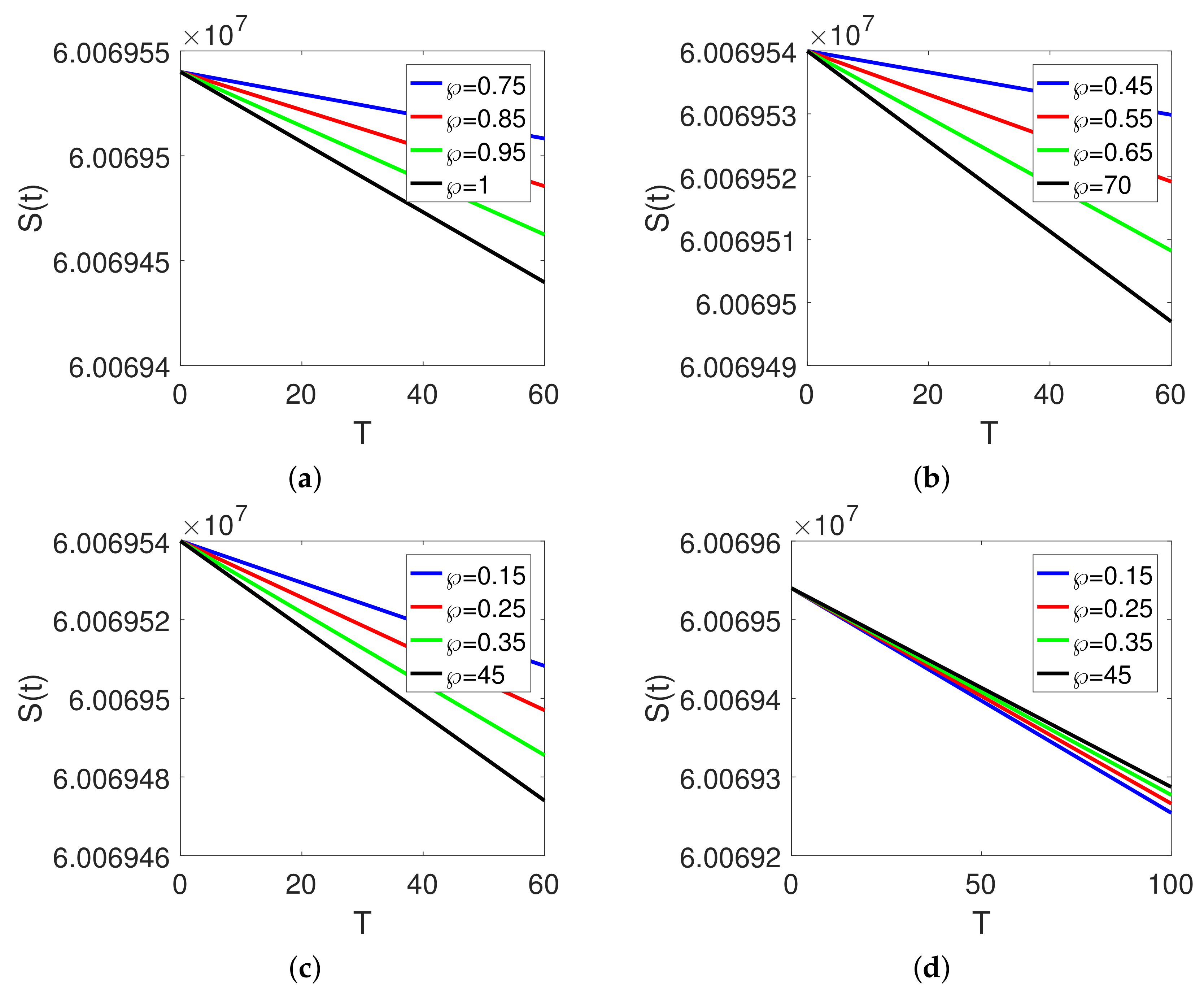
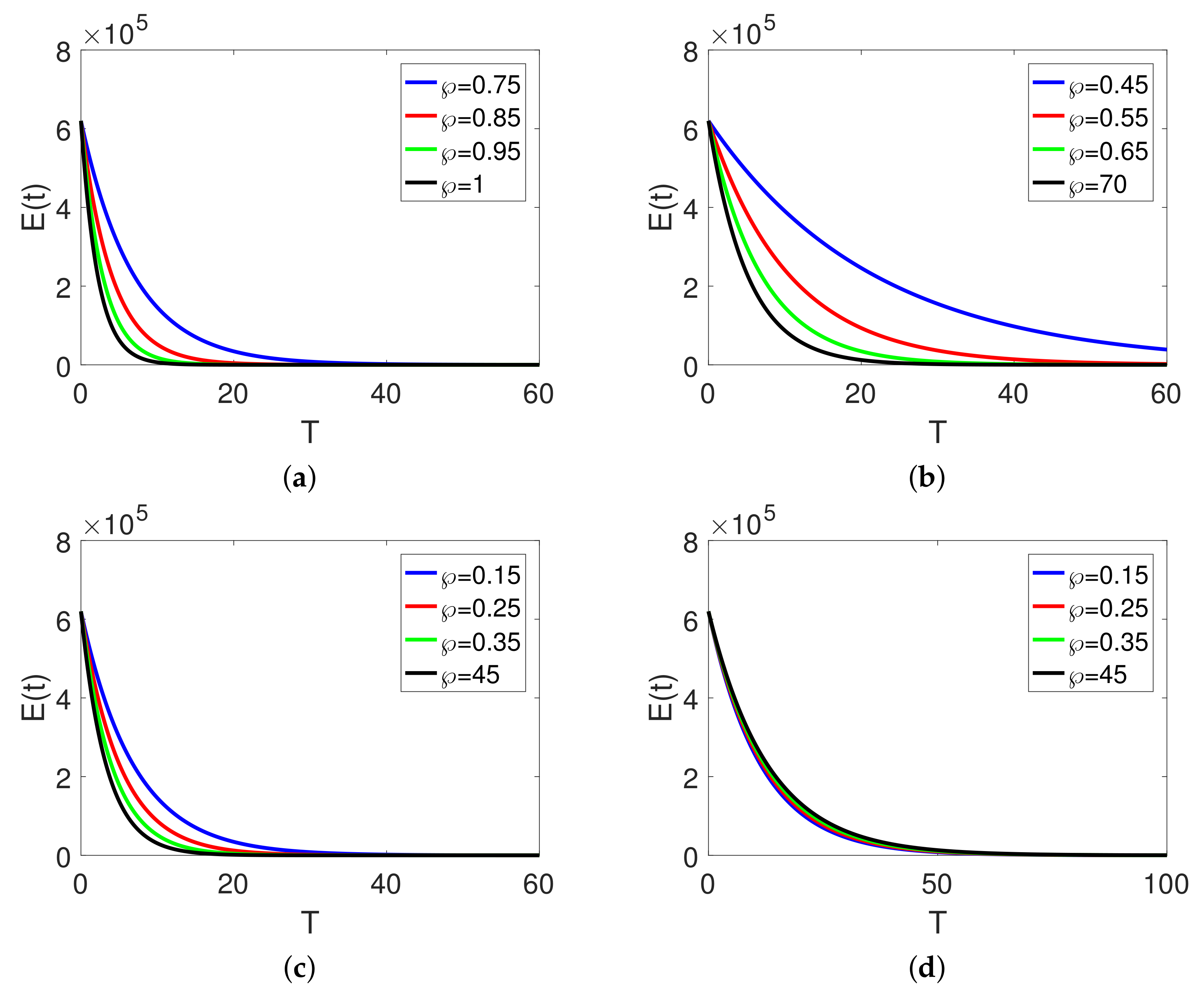
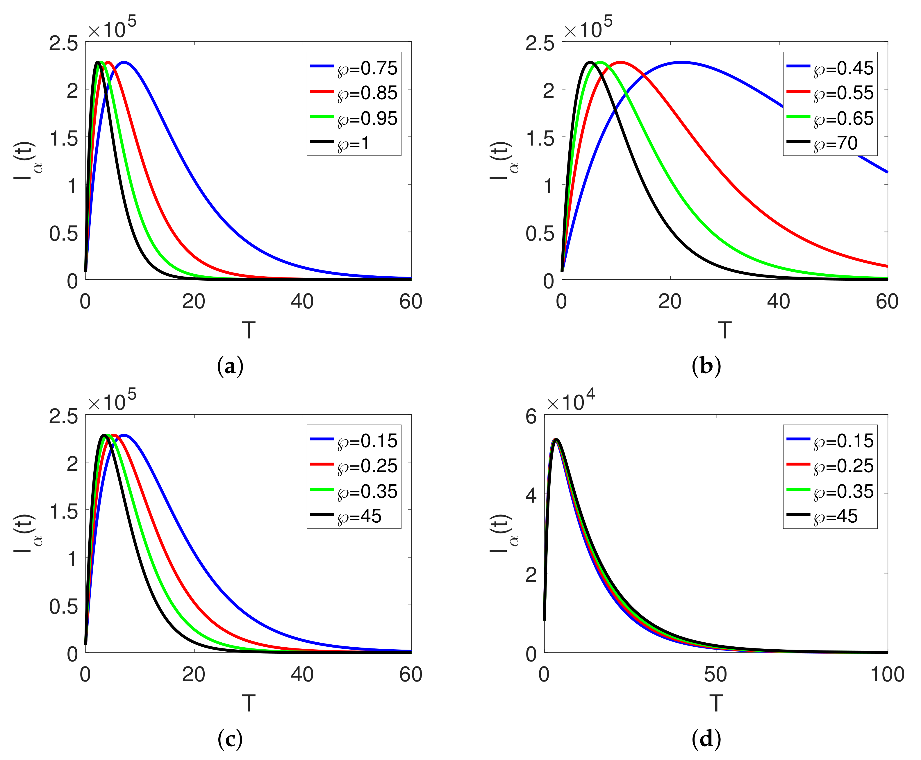
5. Numerical Simulation with Discussion

This section is devoted to the Caputo–Fabrizio derivative model numerical simulation representing the new Omicron virus. We simulate our model for three different fractional orders and time intervals. We take data from [14] for different parameters and compartment of the proposed model as given in Table 2.

Table 2. Initial and parameters numerical values for Omicron virus model [14].

Parameter	Value	Parameter	Value	Parameter	Value
${\mathbb{S}}_0$	$\mathrm{60,069,540}$	u	$\frac{1}{64.38\times 365}$	N	$\mathrm{60,140,000}$
${\mathbb{E}}_0$	$\mathrm{620,000}$	$\alpha$	$0.7999$	$\kappa$	$0.7800$
${\mathbb{I}}_{\alpha \left(0\right)}$	8000	$\tau$	$0.8999$	$\Psi$	$0.9566$
${\mathbb{I}}_{s\left(0\right)}$	360	$\varphi$	$0.0101$	${\Delta }_1$	$0.8447$
${\mathbb{I}}_{O\left(0\right)}$	100	${\Delta }_2$	$0.0200$	${\Delta }_3$	$0.6746$
${\mathbb{R}}_0$	0	${\delta }_1$	$0.0015$

In Figure 1a–d, we draw the dynamics of the susceptible population on three different fractional orders and different time durations. We also variate the step size in the first two graphs, showing that the curves are for away from each other in small step size and vice versa. The class showing decay is transferred to other agents of the system for all different fractional orders and time durations. The decay is greater at the low fractional order and lower at high fractional orders.

Figure 1. Dynamical behavior of susceptible individuals $\mathbb{S}\left(t\right)$ at different arbitrary fractional order ℘ on $[0,T]$, for different times durations.

In Figure 2a–d, we draw the dynamical representation of the exposed population on three different fractional orders and different time durations. We also change the step size in the first two graphs showing that the curves are for away from each other in small step size and vice versa. This class also decreases as it transfers to other compartments of the model for all different fractional orders and time durations. The decrease is greater at low fractional order and lower at high fractional orders.

Figure 2. Dynamical behavior of exposed individuals $\mathbb{E}\left(t\right)$ at different arbitrary fractional order ℘ on $[0,T]$, for different times durations.

Figure 3a–d shows the dynamics of asymptomatic individuals on three different arbitrary orders and time durations. We also change the step size in the first two figures showing that the curves are for away from each other in small step size and vice versa. The population of the said class grows, and after reaching the peak value it declines along with bending at middle. The said class increases by transferring the population from first two classes to it. The increase is greater at high fractional order and lower at low fractional orders while the decrease is the reverse.

Figure 3. Dynamical behavior of asymptomatic individuals ${\mathbb{I}}_{\alpha }\left(t\right)$ at different arbitrary fractional order ℘ on $[0,T]$, for different time durations.

Figure 4a–d shows the dynamical behavior of symptomatic individuals on three different arbitrary orders and time durations for two subintervals showing bending behavior. We change the step size in the first two figures to know about the sensitivity of the model for step size. The population of the said class grows, and after reaching the maximum value it declines and turns at middle. The said class increases by transferring the population from first two classes to it. The increase is greater at high fractional order and lower at low fractional orders while the decrease is the reverse.

Figure 4. Dynamical behavior of symptomatic individuals ${\mathbb{I}}_s\left(t\right)$ at different arbitrary fractional orders ℘ on $[0,T]$, for different times durations.

Figure 5a–d shows the dynamics of Omicron virus infected individuals on four different arbitrary orders and time durations. We change the step size in the first two figures to know about the sensitivity of it. The population of the said class grows and after reaching the maximum value it declines along decay properties at the middle and then stabilizes. The said class increased by transferring the population from first two classes to it in the form of infection cased by Omicron novel infection. The increase is greater at high fractional order and lower at low fractional orders while the decrease is the reverse. With passage of time, the class vanishes or is reduced to minimum or the controlled level.

Figure 5. Dynamical behavior of infection with Omicron virus ${\mathbb{I}}_O\left(t\right)$ at different arbitrary fractional orders r on of $[0,T]$, for different times durations.

Figure 6a–d represents the dynamics of recovery from all types of infection given in the model on three different fractional orders and time durations showing the whole density dynamics. We also fluctuate the step size in the first two figures to know about its sensitivity. The said class grows, and after reaching the maximum value it become stable. The said class increases by transferring the population from all infection classes to it in the form of recovery. The increase is greater at a high fractional order and lower at low fractional orders while the decrease is the reverse.

Figure 6. Dynamical behavior of Recovered individuals $\mathbb{R}\left(t\right)$ at different arbitrary fractional order ℘ on $[0,T]$, for different times durations.

6. Conclusions

We developed a scheme for the fractional dynamics of a non-integer order derivative model of Omicron virus infection by using modified Caputo–Fabrizio fractional operators in the investigated article. The dynamical analysis for the proposed model has been carried out on different fractional orders and time durations. With the help of this article, we will be able to give predictions about infection dynamics at different time intervals with different behaviors. The qualitative techniques for the considered model solution have been developed by using the concept of fixed point theory. In the modified Caputo–Fabrizio framework of order ℘, the numerical solution for the model is evaluated using the Laplace Adomian decomposition procedure. The numerical simulation of all six compartments has been drawn for different data of fractional orders, step size, and time durations. This type of analysis can be applied to real-world dynamical phenomena where change or variation occurs. This investigation is a more realistic approach as the dynamics are changing differently at different time durations. Such an analysis describes the total property spectrum, which is very rarely given in both integer and fractional order deterministic and stochastic problems.

References

1. Omicron Variant: What You Need to Know. Available online: https://www.cdc.gov/coronavirus/2019-ncov/variants/omicron-variant.html (accessed on 23 January 2022).
2. Khan, M.A.; Atangana, A. Modeling the dynamics of novel coronavirus (2019-nCov) with fractional derivative. Alex. Eng. J. 2020, 59, 2379–2389. [Google Scholar] [CrossRef]
3. Ullah, S.; Khan, M.A. Modeling the impact of non-pharmaceutical interventions on the dynamics of novel coronavirus with optimal control analysis with a case study. Chaos Solitons Fractals 2020, 139, 110075. [Google Scholar] [CrossRef] [PubMed]
4. Khan, M.A.; Atangana, A.; Alzahrani, E.; Fatmawati. The dynamics of COVID-19 with quarantined and isolation. Adv. Differ. Equ. 2020, 2020, 425. [Google Scholar] [CrossRef] [PubMed]
5. Atangana, A. Modelling the spread of COVID-19 with new fractal-fractional operators: Can the lockdown save mankind before vaccination? Chaos Solitons Fractals 2020, 136, 109860. [Google Scholar] [CrossRef] [PubMed]
6. López, L.; Rodo, X. A modified SEIR model to predict the COVID-19 outbreak in Spain and Italy: Simulating control scenarios and multi-scale epidemics. Results Phys. 2021, 21, 103746. [Google Scholar] [CrossRef]
7. Ayinde, K.; Lukman, A.F.; Rauf, R.I.; Alabi, O.O.; Okon, C.E.; Ayinde, O.E. Modeling Nigerian COVID-19 cases: A comparative analysis of models and estimators. Chaos Solitons Fractals 2020, 138, 109911. [Google Scholar] [CrossRef] [PubMed]
8. Aba Oud, M.A.; Ali, A.; Alrabaiah, H.; Ullah, S.; Khan, M.A.; Islam, S. A fractional order mathematical model for COVID-19 dynamics with quarantine, isolation, and environmental viral load. Adv. Differ. Equ. 2021, 2021, 106. [Google Scholar] [CrossRef]
9. Khan, M.A.; Ullah, S.; Kumar, S. A robust study on 2019-nCOV outbreaks through non-singular derivative. Eur. Phys. J. Plus 2021, 136, 168. [Google Scholar] [CrossRef]
10. Chu, Y.M.; Ali, A.; Khan, M.A.; Islam, S.; Ullah, S. Dynamics of fractional order COVID-19 model with a case study of Saudi Arabia. Results Phys. 2021, 21, 103787. [Google Scholar] [CrossRef]
11. Kucharski, A.J.; Funk, S.; Eggo, R.M.; Mallet, H.-P.; Edmunds, W.J.; Nilles, E.J. Transmission dynamics of Zika virus in island populations: A modelling analysis of the 2013–14 French Polynesia outbreak. PLoS Negl. Trop. Dis. 2016, 10, e0004726. [Google Scholar] [CrossRef] [Green Version]
12. Bonyah, E.; Okosun, K.O. Mathematical modeling of Zika virus. Asian Pac. J. Trop. Dis. 2016, 6, 637–679. [Google Scholar] [CrossRef]
13. Bonyah, E.; Khan, M.A.; Okosun, K.O.; Islam, S. A theoretical model for Zika virus transmission. PLoS ONE 2017, 12, e0185540. [Google Scholar] [CrossRef] [PubMed]
14. Khan, M.A.; Atangana, A. Mathematical modeling and analysis of COVID-19: A study of new variant Omicron. Phys. A 2022, 599, 127452. [Google Scholar] [CrossRef] [PubMed]
15. Atangana, A.; Baleanu, D. New fractional derivatives with non-local and non-singular kernel: Theory and application to heat transfer model. Therm. Sci. 2016, 20, 763–769. [Google Scholar] [CrossRef]
16. Goufo, E.F.D. Application of the Caputo-Fabrizio fractional derivative without singular kernel to Korteweg-de Vries-Burgers equation. Math. Model. Anal. 2016, 21, 188–198. [Google Scholar] [CrossRef]
17. Goufo, E.F.D. A bio mathematical view on the fractional dynamics of cellulose degradation. Fract. Calc. Appl. Anal. 2015, 18, 554–564. [Google Scholar] [CrossRef]
18. Atangana, A. Extension of rate ofchange concept:from local to nonlocal operators with applications. Results Phys. 2020, 19, 103515. [Google Scholar] [CrossRef]
19. Atangana, A.; Araz, S.I. Nonlinear equations with global differential and integral operators:existence, uniqueness with application to epidemiology. Results Phys. 2021, 20, 103593. [Google Scholar] [CrossRef]
20. Xu, C.; Liao, M.; Li, P.; Yuan, S. Impact of leakage delay on bifurcation in fractional-order complex-valued neural networks. Chaos Solitons Fractals 2021, 142, 110535. [Google Scholar] [CrossRef]
21. Kabunga, S.K.; Goufo, E.F.D.; Tuong, V.H. Analysis and simulation of a mathematical model of tuberculosis transmission in democratic Republic of the Congo. Adv. Differ. Equ. 2020, 2020, 642. [Google Scholar] [CrossRef]
22. Atangana, A.; Araz, S.I. Mathematical model of COVID-19 spread in Turkey and South Africa: Theory, methods and applications. Adv. Differ. Equ. 2020, 2020, 659. [Google Scholar] [CrossRef] [PubMed]
23. Xu, C.; Liu, Z.X.; Liao, M.X.; Yao, L.Y. Theoretical analysis and computer simulations of a fractional order bank data model incorporating two unequal time delays. Expert Syst. Appl. 2022, 199, 116859. [Google Scholar] [CrossRef]
24. Liu, P.; ur Rahman, M.; Din, A. Fractal fractional based transmission dynamics of COVID-19 epidemic model. Comput. Methods Biomech. Biomed. Eng. 2022, 1–18. [Google Scholar] [CrossRef] [PubMed]
25. Shen, W.Y.; Chu, Y.M.; ur Rahman, M.; Mahariq, I.; Zeb, A. Mathematical analysis of HBV and HCV co-infection model under nonsingular fractional order derivative. Results Phys. 2021, 28, 104582. [Google Scholar] [CrossRef]
26. Haidong, Q.; ur Rahman, M.; Arfan, M.; Salimi, M.; Salahshour, S.; Ahmadian, A. Fractal–fractional dynamical system of Typhoid disease including protection from infection. Eng. Comput. 2021, 1–10. [Google Scholar] [CrossRef]
27. Xu, C.; ur Rahman, M.; Baleanu, D. On fractional-order symmetric oscillator with offset-boosting control. Nonlinear Anal. Model. Control. 2022, 27, 1–15. [Google Scholar] [CrossRef]
28. Atangana, A.; Araz, S.I. New concept in calculus: Piecewise differential and integral operators. Chaos Soliton. Fract. 2021, 145, 110638. [Google Scholar] [CrossRef]
29. Arfan, M.; Shah, K.; Ullah, A.; Salahshour, S.; Ahmadian, A.; Ferrara, M. A novel semi-analytical method for solutions of two dimensional fuzzy fractional wave equation using natural transform. Discret. Contin. Dyn. Syst.-S 2022, 15, 315–338. [Google Scholar] [CrossRef]
30. ur Rahman, M.; Arfan, M.; Shah, Z.; Alzahrani, E. Evolution of fractional mathematical model for drinking under Atangana-Baleanu Caputo derivatives. Phys. Scr. 2021, 96, 115203. [Google Scholar] [CrossRef]
31. ur Rahman, M.; Arfan, M.; Deebani, W.; Kumam, P.; Shah, Z. Analysis of time-fractional Kawahara equation under Mittag-Leffler Power Law. Fractals 2022, 30, 2240021. [Google Scholar] [CrossRef]
32. Caputo, M.; Fabrizio, M. A new Definition of Fractional Derivative without Singular Kernel. Prog. Fract. Differ. Appl. 2015, 1, 73–85. [Google Scholar]
33. Caputo, M.; Fabrizio, M. On the singular kernels for fractional derivatives. Some applications to partial differential equations. Progr. Fract. Differ. Appl. 2021, 7, 79–82. [Google Scholar]