Solutions of General Fractional-Order Differential Equations by Using the Spectral Tau Method

Abstract

Here, in this article, we investigate the solution of a general family of fractional-order differential equations by using the spectral Tau method in the sense of Liouville–Caputo type fractional derivatives with a linear functional argument. We use the Chebyshev polynomials of the second kind to develop a recurrence relation subjected to a certain initial condition. The behavior of the approximate series solutions are tabulated and plotted at different values of the fractional orders $\nu$ and $\alpha$. The method provides an efficient convergent series solution form with easily computable coefficients. The obtained results show that the method is remarkably effective and convenient in finding solutions of fractional-order differential equations.

1. Introduction

Fractional-order differential equations have gained interest in many different research areas, especially in engineering problems. As most fractional differential equations do not have analytic solutions, we have to use different methods to convert such differential equations to more accurate equations for which we can then use various approximation and numerical techniques. The spectral Tau and collocation methods are widely used for solving fractional differential equations (FDE). The operational approach of the Tau method was employed for solving fractional problems in [1].

There is a numerical method based on the Tau method, which was provided for FDE [2]. In 2013, Ren et al. [3] introduced an efficient method for solving the space fractional diffusion equations based on the shifted Chebyshev-Tau idea presented. As far as we know, the Tau method is very effective for constant coefficient nonlinear problems, but it is not generally used for nonlinear FDE [4]. The spectral method was developed through the numerical solutions of differential equations of fractional order. It gives higher accuracy than other numerical methods and has plenty of applications in both physical and mathematical problems.

The first kind of Chebyshev polynomials, written as $T_{{\ell }_1}\left(\zeta \right)$, is the most common basis function that will be used for the spectral method. The spectral method is used to solve delay differential equations of integer order depending on Bernoulli polynomials [5], Chebyshev polynomials [6], special Bessel-type polynomials [7], Legendre wavelet [8], and Taylor series and hybrid of block-pulse functions [9]. Moreover, the numerical solutions of fractional-order delay differential equations (FODDEs) can be found in the literature (see, for example [10,11,12,13,14,15,16,17,18,19,20]). Differential equations of advanced argument were contributed and compared to delay differential equations and there are many developments that can be found in [21,22,23,24].

It is worth observing that the general form of argument has a mixed-type equation (see [25]). Recently, the backward substitution method was used by Reutskiy [26] for multi-point problems with linear Fredholm–Volterra differential equations of the neutral integro type. More recently, Ramadan et al. [27] reported that a solution of the generalized delay differential equations of the pantograph type has linear functional arguments. All works are considered as generalizations of advanced and delay differential equations, which is a unification with derivatives of integer order.

In this investigation, we introduce a new generalized form of the delay and advanced differential equations involving derivatives of fractional order. The problem is determined by the solution of general fractional differential equations (SGFDEs) with linear functional argument via the method of spectral Tau [28]. This is defined as follows:

$$\rho \left(\zeta ,\sigma \left(\zeta \right),D^{v_{\iota }}\sigma (p_{\iota }\zeta +{\xi }_{\iota }),{\sigma }^{\left(\iota \right)}(q_{\iota }\zeta +{\mathrm{z}}_{\iota })\right)=0,$$

(1)

with the following condition:

$${\sigma }^{\left(\iota \right)}\left(0\right)={\mathsf{c}}_{\iota },$$

(2)

for ${\ell }_1-1<v_{\iota }<{\ell }_1,v_{\iota }>0,\iota =0,1,2,\dots ,{\ell }_1,a\le \zeta \le b$ and $q_{\iota },p_{\iota },{\xi }_{\iota },{\mathrm{z}}_{\iota }$ are all in $\mathbb{R}$.

It can be seen that (1) and (2) are a general form of the fractional-order differential equation. They focus on linear equations of a linear function $f\left(x\right)$, where the linear fractional argument is established to deal with a generalized form by the method of spectral Tau. The linear fractional argument with the Tau method are together used as a new matrix discretization method.

The integral and derivative operators of fractional calculus generalize those of the standard calculus of integer order. Their concept was developed fairly widely with the development of classical operators (see, for details [29,30]). Fractional integrals and fractional derivatives have been applied in many areas of mathematical, physical and engineering sciences during the last few decades (see [31]). Before the nineteenth century, no analytical method was available for fractional-order differential equations. However, in 2009, the first analytical method was proposed in [32] via the variation iteration method (VIM).

Various approaches are known for solving fractional-order differential equations, such as, for example, linear and nonlinear viscoelastic models with fractional derivatives, nonlinear differential equations of fractional order, linear fractional partial differential equations arising in fluid mechanics, and the fractional heat and wave-like equations with variable coefficients. The collocation methods for solving several kinds of FDEs are based on various kinds of orthogonal functions and their variants. We only focus here on the case when the order of the derivative involved is a fixed constant. Our main motivation here is, therefore, to solve variable-order linear and nonlinear multiterm FDEs numerically via the second kind of Chebyshev polynomials.

We derive a differential linear fractional argument based on the second kind of Chebyshev polynomials. We use the linear fractional argument to transform the equation into the products of dependent matrices. This can also be viewed as an algebraic system by using the collocation points. Solving the algebraic system can reduce the size of the computational work, while accurately providing the series solution. Differential equations of fractional order are used to model a variety of systems of real-world physical problems of which the important applications can be found in [6].

Several real-world phenomena emerging in engineering and science fields can be demonstrated successfully by developing a model using the theory of fractional calculus. The exact or semi-analytical solution to many physical problems can be understood by studying a physical phenomenon’s future, current and historical states. The spectral Tau method is used for solving the solution of the general fractional-order differential equation. This can be used to find the solution of the general fractional-order differential equation with the Chebyshev polynomials of the first kind. Instead, in this article, we apply the Chebyshev polynomials of the second kind. Accordingly, this finding aims to extend, by applying the Chebyshev polynomial of the second kind, and intends to find solutions of fractional-order differential equations using the spectral Tau-method.

The outline of our investigation is arranged as follows. Section 2 recalls mathematical preliminaries and prepares the method to reach the numerical results as follows: Section 2.1 recalls the Liouville–Caputo type fractional derivatives, Section 2.2 recalls the second kind of the Chebyshev polynomials and their major properties, and Section 2.3 prepares linear fractional argument formulations. The methodology is then applied in Section 3 by examining the proposed method and applying it on the required FODDE. The method of solution is proposed in Section 4 together with its error estimation. Section 5 presents the exact and approximate solutions of five examples of time-fractional diffusion equations. Section 6 finally provides some concluding remarks.

2. Mathematical Formulation for the Main Results

2.1. Liouville–Caputo Type Fractional Derivatives

In the existing literature, we can find many different ways to define fractional-order derivatives (see, for example [33]; see also the recently published works [34,35,36,37]). Here, in this article, we chose to use the Liouville–Caputo type fractional derivative of order v, which is defined by

$$D^{v}g\left(\zeta \right)=\frac{1}{\mathsf{\Gamma }({\ell }_2-v)}{\int }_0^{\zeta }\frac{g^{\left({\ell }_2\right)}\left(t\right)}{{(\zeta -t)}^{v-{\ell }_2+1}}dt\left(\zeta >0;{\ell }_2-1<v<{\ell }_2;{\ell }_2\in \mathbb{N}\right),$$

(3)

where $\mathbb{N}$ denotes the set of positive integers. Furthermore, these are some of its essential properties:

• $D^v(\lambda g\left(\zeta \right)+\mathrm{fi}h\left(\zeta \right))=\lambda D^{v}g\left(\zeta \right)+\mathrm{fi}{D}^{v}h\left(\zeta \right)$ for each constant $\lambda$ and $\mathrm{fi}$;
• $D^v\left(\mathrm{a}\mathrm{constant}\right)=0$;
• For ${\ell }_1\in {\mathbb{N}}_0$, we have

  $$D^v{\zeta }^{{\ell }_1}=\left\{\begin{array}{cc}{\displaystyle \frac{\mathsf{\Gamma }({\ell }_1+1)}{\mathsf{\Gamma }({\ell }_1+1-\nu )}},\hfill & \mathrm{for}{\ell }_1\in {\mathbb{N}}_0\mathrm{and}{\ell }_1⩾\left[\nu \right];\hfill \\ 0,\hfill & \mathrm{for}{\ell }_1\in {\mathbb{N}}_0\mathrm{and}{\ell }_1<\left[\nu \right],\hfill \end{array}\right.$$

  where ${\mathbb{N}}_0=\mathbb{N}\cup \left\{0\right\}.$

2.2. Second Kind Chebyshev Polynomial

In this section, we recall the second kind Chebyshev polynomial of order ${\ell }_1$ and some of its properties (see [6]), which is defined as follows:

$${\mathrm{Y}}_{{\ell }_1}\left(\zeta \right)=\frac{sin\left(({\ell }_1+1)\phi \right)}{sin\phi },$$

(4)

where $\zeta =cos\phi$ and $0\le \phi \le \pi$. Then

$$\begin{array}{cc}\hfill {\mathrm{Y}}_0\left(\zeta \right)& =\frac{sin\left(\right(0+1\left)\phi \right)}{sin\phi }=\frac{sin\phi }{sin\phi }=1,\hfill \\ \hfill {\mathrm{Y}}_1\left(\zeta \right)& =\frac{sin\left(\right(1+1\left)\phi \right)}{sin\phi }=2cos\phi =2\zeta ,\hfill \\ \hfill {\mathrm{Y}}_2\left(\zeta \right)& =\frac{sin\left(\right(2+1\left)\phi \right)}{sin\phi }=\frac{sin3\phi }{sin\phi }=3-4{sin}^2\phi =4{cos}^2\zeta -1=4{\zeta }^2-1.\hfill \end{array}$$

Since

$${\mathrm{Y}}_{{\ell }_1+1}\left(\zeta \right)+{\mathrm{Y}}_{{\ell }_1-1}\left(\zeta \right)=\frac{sin\left(({\ell }_1+2)\phi \right)+sin\phi }{sin\phi }=\frac{2sin\left(({\ell }_1+1)\phi \right)cos\phi }{sin\phi }=2\zeta {\mathrm{Y}}_{{\ell }_1}\left(\zeta \right).$$

It follows that

$${\mathrm{Y}}_{{\ell }_1+1}\left(\zeta \right)=2\zeta {\mathrm{Y}}_{{\ell }_1}\left(\zeta \right)-{\mathrm{Y}}_{{\ell }_1-1}\left(\zeta \right).$$

(5)

So, we have

$$\begin{array}{cc}\hfill {\mathrm{Y}}_3\left(\zeta \right)& =8{\zeta }^3-4\zeta .\hfill \\ \hfill {\mathrm{Y}}_4\left(\zeta \right)& =16{\zeta }^4-12{\zeta }^2+1.\hfill \\ \hfill {\mathrm{Y}}_5\left(\zeta \right)& =32{\zeta }^5-32{\zeta }^3+6\zeta .\hfill \\ \hfill {\mathrm{Y}}_6\left(\zeta \right)& =64{\zeta }^6-80{\zeta }^4+24{\zeta }^2-1.\hfill \end{array}$$

Hence, for ${\ell }_1=1,2,\dots$, leading coefficient of ${\mathrm{Y}}_{{\ell }_1}\left(\zeta \right)=2^{{\ell }_1}$, constant term of ${\mathrm{Y}}_{2\kappa }\left(\zeta \right)={(-1)}^{\kappa }$ and the coefficients of $\zeta$ in ${\mathrm{Y}}_{2\kappa +1}\left(\zeta \right)={(-1)}^{\kappa }(2\kappa +2)\zeta$. Therefore, one can have

$$\begin{array}{cc}\hfill 1& ={\mathrm{Y}}_0\left(\zeta \right),\hfill \\ \hfill \zeta & =\frac{1}{2}{\mathrm{Y}}_1\left(\zeta \right),\hfill \\ \hfill {\zeta }^2& =\frac{1}{2^2}\left[{\mathrm{Y}}_0\left(\zeta \right)+{\mathrm{Y}}_2\left(\zeta \right)\right],\hfill \\ \hfill {\zeta }^3& =\frac{1}{2^3}\left[2{\mathrm{Y}}_1\left(\zeta \right)+{\mathrm{Y}}_3\left(\zeta \right)\right].\hfill \end{array}$$

On the other hand, we can express the Chebyshev polynomials ${\mathrm{Y}}_{{\ell }_1}\left(\zeta \right)$ as follows (see [27]):

$${\mathrm{Y}}_{{\ell }_1}\left(\zeta \right)=\sum _{{\ell }_2=0}^{\left[\frac{{\ell }_1-1}{2}\right]}\frac{{(-1)}^{{\ell }_2}{\ell }_1!}{(2{\ell }_2+1)!({\ell }_1-2{\ell }_2-1)!}{(1-{\zeta }^2)}^{{\ell }_2+\frac{1}{2}}{\zeta }^{{\ell }_1-2{\ell }_2-1}.$$

(6)

Now, we have

$$\begin{array}{cc}\hfill {\mathrm{Y}}_{{\ell }_1}\left(\zeta \right)& =sin\left({\ell }_1{cos}^{-1}\zeta \right)=sin{\ell }_1\phi \hfill \\ \hfill & =\frac{1}{2i}|e^{i{\ell }_1\phi }-e^{-i{\ell }_1\phi }|\hfill \\ \hfill & =\frac{1}{2i}\left[{(cos\phi +isin\phi )}^{{\ell }_1}-{(cos\phi -isin\phi )}^{{\ell }_1}\right],\hfill \end{array}$$

which implies that

$${\mathrm{Y}}_{{\ell }_1}\left(\zeta \right)=\frac{1}{2i}\left[{\{\zeta +i\sqrt{1-{\zeta }^2}\}}^{{\ell }_1}-{\{\zeta -i\sqrt{1-{\zeta }^2}\}}^{{\ell }_1}\right].$$

Since $\zeta =cos\phi$ and ${sin}^2\phi +{cos}^2\phi =1$, it follows that

$$\begin{array}{cc}\hfill {sin}^2\phi +{\zeta }^2& =1\hfill \\ \hfill {sin}^2\phi & =1-{\zeta }^2\hfill \\ \hfill sin\phi & =\sqrt{1-{\zeta }^2}\hfill \\ \hfill & =\frac{1}{2i}\left[\sum _{{\ell }_2=0}^{{\ell }_1}{\ell }_1{C}_{{\ell }_2}{\zeta }^{{\ell }_1-{\ell }_2}{\left\{-i\sqrt{1-{\zeta }^2}\right\}}^{{\ell }_2}-\sum _{{\ell }_2=0}^{{\ell }_1}{\ell }_1{C}_{{\ell }_2}{\zeta }^{{\ell }_1-{\ell }_2}{\left\{i\sqrt{1-{\zeta }^2}\right\}}^{{\ell }_1}\right]\hfill \\ \hfill & =\frac{1}{2i}\left[\sum _{{\ell }_2=0}^{{\ell }_1}{\ell }_1{C}_{{\ell }_2}{\zeta }^{{\ell }_1-{\ell }_2}\left\{1^{{\ell }_2}-{(-1)}^{{\ell }_2}\right\}{i}^{{\ell }_2}{(1-{\zeta }^2)}^{\frac{{\ell }_2}{2}}\right],\hfill \end{array}$$

where

$$C_{{\ell }_2}^{{\ell }_1}=\left(\genfrac{}{}{0pt}{}{{\ell }_1}{{\ell }_2}\right)=\frac{{\ell }_1!}{({\ell }_1-{\ell }_2){\ell }_2!}.$$

$Casei$: If ${\ell }_2$ is even, then ${\mathrm{Y}}_{{\ell }_1}\left(\zeta \right)=0$.

$Caseii$: If ${\ell }_2$ is odd, then ${\ell }_2=2r+1$ for some $r\in \mathbb{Z}$.

Since ${\ell }_2\le {\ell }_1,r\le \frac{{\ell }_1-1}{2}$, then $\mathrm{Y}\left(\zeta \right)$ can be expressed as the following general matrix:

$$\mathrm{Y}\left(\zeta \right)=X\left(\zeta \right)M^T,$$

(7)

where the matrices $\mathrm{Y}\left(\zeta \right)$ and $X\left(\zeta \right)$ are given by

$$\mathrm{Y}\left(\zeta \right)=\left[{\mathrm{Y}}_0\left(\zeta \right){\mathrm{Y}}_1\left(\zeta \right)\cdots {\mathrm{Y}}_{\mu }\left(\zeta \right)\right],X\left(\zeta \right)=\left[X^0\left(\zeta \right)X^1\left(\zeta \right)\cdots X^{\mu }\left(\zeta \right)\right],$$

respectively, and M is lower triangle $({\ell }_1+1)\times ({\ell }_1+1)$ constant matrix given by

$$\begin{array}{c}\hfill M=\left(\begin{array}{ccccccc}\left(\genfrac{}{}{0pt}{}{0}{0}\right)& 0& 0& 0& \cdots & 0& 0\\ 0& 2\left(\genfrac{}{}{0pt}{}{1}{0}\right)& 0& 0& \cdots & 0& 0\\ (-1)2^0\left(\genfrac{}{}{0pt}{}{1}{0}\right)& 0& 2^2\left(\genfrac{}{}{0pt}{}{2}{0}\right)& 0& \cdots & 0& 0\\ 0& (-1)2^r\left(\genfrac{}{}{0pt}{}{2}{1}\right)& 0& 2^3\left(\genfrac{}{}{0pt}{}{3}{0}\right)& & 0& 0\\ ⋮& ⋮& ⋮& ⋮& & ⋮& ⋮\\ {(-1)}^r{2}^0\left(\genfrac{}{}{0pt}{}{2}{1}\right)& 0& {(-1)}^{r-1}{2}^2\left(\genfrac{}{}{0pt}{}{r+1}{r-1}\right)& 0& \cdots & 2^{2r}\left(\genfrac{}{}{0pt}{}{2r}{0}\right)& 0\\ 0& {(-1)}^r{2}^r\left(\genfrac{}{}{0pt}{}{r-1}{n}\right)& 0& {(-1)}^{r-1}{2}^3\left(\genfrac{}{}{0pt}{}{r+2}{r-1}\right)& \cdots & 0& 2^{2r+1}\left(\genfrac{}{}{0pt}{}{2r+1}{0}\right)\end{array}\right)\end{array}$$

(8)

Here, we deal with the last row for odd values of ${\ell }_2=2r+1$. Otherwise, it becomes $M({\ell }_2=2r)$. Now, from (7) we can obtain the $\kappa \mathrm{th}$ derivative of the matrix $\mathrm{Y}\left(\zeta \right)$ as

$${\mathrm{Y}}^{\left(\kappa \right)}\left(\zeta \right)=X^{\left(\kappa \right)}\left(\zeta \right)M^T\left(\mathrm{for}\kappa =0,1,2,\dots \right).$$

(9)

2.3. Linear Fractional Arguments

In this section, we attempt to find the generalization of linear functional arguments for ${\mathrm{Y}}^{\left(\kappa \right)},\mathrm{Y}(\zeta -\mathrm{z}),{\mathrm{Y}}^{\left(s\right)}(\zeta -\mathrm{z}),D^{v_{\iota }}\mathrm{Y}\left(\zeta \right)$ and ${\mathrm{Y}}^{\left({\alpha }_{\iota }\right)}(\zeta -\mathrm{z})$ by using relations (6) and (7) with respect to fractional calculus.

Following [10], we see that the $\kappa \mathrm{th}$ derivative of $\mathrm{Y}\left(\zeta \right)$ is as follows:

$${\chi }^{\left(\kappa \right)}\left(\zeta \right)=\chi \left(\zeta \right)H^{\kappa },$$

(10)

where the square matrix H is given by

$$H=\left(\begin{array}{ccccc}0& 1& 0& \cdots & 0\\ 0& 0& 2& \cdots & 0\\ ⋮& ⋮& ⋮& & ⋮\\ 0& 0& 0& \cdots & \mu \\ 0& 0& 0& \cdots & 0\end{array}\right).$$

In addition, the row vector $\mathrm{Y}(q_{\iota }\zeta +{\mathrm{z}}_{\iota })$ cab be expressed as

$$\mathrm{Y}(q_{\iota }\zeta +{\mathrm{z}}_{\iota })=\chi (q_{\iota }\zeta +{\mathrm{z}}_{\iota })M^T.$$

(11)

The κth derivative of $\mathrm{Y}(q_{\iota }\zeta +{\mathrm{z}}_{\iota })$ cab be expressed as

$${\mathrm{Y}}^{\left(\kappa \right)}(q_{\iota }\zeta +{\mathrm{z}}_{\iota })={\chi }^{\left(\kappa \right)}(q_{\iota }\zeta +{\mathrm{z}}_{\iota })M^T=\chi \left(\zeta \right)B{\mathrm{z}}_{\iota }{H}^{\kappa }{\left(M\vartheta q_{\iota }\right)}^T,$$

(12)

where the elements of the diagonal matrix $\vartheta q_{\iota }$ are as follows:

$${\vartheta }_{rs}=\left\{\begin{array}{cc}0,\hfill & forr\ne s;\hfill \\ q_{\iota }^r,\hfill & forr=s,\hfill \end{array}\right.$$

(13)

and

$$B_{{\mathrm{z}}_{\iota }}=\left(\begin{array}{ccccc}1{\left({\mathrm{z}}_{\iota }\right)}^0& 1{\left({\mathrm{z}}_{\iota }\right)}^1& 1{\left({\mathrm{z}}_{\iota }\right)}^2& \cdots & 1{\left({\mathrm{z}}_{\iota }\right)}^{\mu }\\ 0& 1{\left({\mathrm{z}}_{\iota }\right)}^0& 1{\left({\mathrm{z}}_{\iota }\right)}^1& \cdots & \left(\genfrac{}{}{0pt}{}{\mu }{1}\right){\left({\mathrm{z}}_{\iota }\right)}^{\mu -1}\\ 0& 0& 1{\left({\mathrm{z}}_{\iota }\right)}^0& \cdots & \left(\genfrac{}{}{0pt}{}{\mu }{2}\right){\left({\mathrm{z}}_{\iota }\right)}^{\mu -2}\\ ⋮& ⋮& ⋮& & ⋮\\ 0& 0& 0& \cdots & 1{\left({\mathrm{z}}_{\iota }\right)}^0\end{array}\right).$$

Finally, the $v_i^{\mathrm{th}}$ order fractional derivative of $\mathrm{Y}\left(\zeta \right)$ takes the form

$$\begin{array}{cc}\hfill & D^{v_{\iota }}\mathrm{Y}\left(\zeta \right)={\chi }_{v_{\iota }}\left(\zeta \right)H_{v_{\iota }}{M}^T,\hfill \end{array}$$

(14)

where $0<v_{\iota }<1$,

$$\begin{array}{cc}\hfill & {\chi }_{v_{\iota }}\left(\zeta \right)=[0,{\zeta }^{1-v_{\iota }},{\zeta }^{2-v_{\iota }},\dots ,{\zeta }^{\mu -v_{\iota }}],\hfill \end{array}$$

(15)

and

$$\begin{array}{cc}\hfill H_{v_{\iota }}& =\left(\begin{array}{ccccc}0& 0& 0& \cdots & 0\\ 0& \frac{\mathsf{\Gamma }\left(2\right)}{\mathsf{\Gamma }(2-v_{\iota })}& 0& \cdots & 0\\ 0& 0& \frac{\mathsf{\Gamma }\left(3\right)}{\mathsf{\Gamma }(3-v_{\iota })}& \cdots & 0\\ ⋮& ⋮& ⋮& & ⋮\\ 0& 0& 0& \cdots & \frac{\mathsf{\Gamma }(\mu +1)}{\mathsf{\Gamma }(\mu +1-v_{\iota })}\end{array}\right).\hfill \end{array}$$

(16)

3. Theoretical Analysis Applied to FODDE

This section is dedicated to obtaining the general linear fractional argument for all terms (1) and (2).

First, we consider the general FODDE:

$$\begin{array}{c}\hfill \sum _{\iota =0}^{n_1}{Q}_{\iota }\left(\zeta \right)D^{v_{\iota }}y\left(\zeta \right)+\sum _{j=0}^{n_2}{P}_j\left(\zeta \right)D^{{\alpha }_j}y(\zeta -\mathrm{z})+\sum _{\kappa =0}^{n_3}{Q}_{\kappa }^{*}\left(\zeta \right)y^{\left(\kappa \right)}\left(\zeta \right)+\sum _{s=0}^{n_4}{P}_s^{*}\left(\zeta \right)y^{\left(s\right)}(\zeta -\mathrm{z})=g\left(\zeta \right),\end{array}$$

(17)

with

$$y^{\iota }\left(0\right)={\mathsf{c}}_{\iota }\left(\mathrm{for}\iota =0,1,2,\dots ,{\ell }_2-1\right),$$

(18)

where $Q_{\iota }\left(\zeta \right),Q_{\kappa }^{*}\left(\zeta \right),P_j\left(\zeta \right)$ and $P_s^{*}\left(\zeta \right)$ are known functions, and ${\ell }_2$ is either the highest integer order greater than the fractional derivative, or the greatest integer order derivative that exists.

We rewrite (17) as

$$D\left(\zeta \right)+F\left(\zeta \right)+L\left(\zeta \right)+H\left(\zeta \right)=g\left(\zeta \right),$$

(19)

where

$$\begin{array}{cc}\hfill D\left(\zeta \right)& =\sum _{\iota =0}^{n_1}{Q}_{\iota }\left(\zeta \right)D^{v_{\iota }}y\left(\zeta \right),F\left(\zeta \right)=\sum _{j=0}^{n_2}{P}_j\left(\zeta \right)D^{{\alpha }_j}y(\zeta -\mathrm{z}),\hfill \\ \hfill L\left(\zeta \right)& =\sum _{\kappa =0}^{n_3}{Q}_{\kappa }^{*}\left(\zeta \right)y^{\left(\kappa \right)}\left(\zeta \right),H\left(\zeta \right)=\sum _{s=0}^{n_4}{P}_s^{*}\left(\zeta \right)y^{\left(s\right)}(\zeta -\mathrm{z}).\hfill \end{array}$$

Therefore, we can propose the approximate solution via the Chebyshev polynomial of the second kind as follows:

$$y\left(\zeta \right)\cong y_{\mu }\left(\zeta \right)=\sum _{\mathrm{z}=0}^{\mu }{a}_{\mathrm{z}}{\mathrm{Y}}_{\mathrm{z}}\left(\zeta \right),$$

(20)

where the coefficients $a_{\mathrm{z}}$ are given by

$$a_{\iota }=\frac{2}{\pi }{\int }_{-1}^1{\mathrm{Y}}_{\iota }\left(\zeta \right)Y_{\mu }\left(\zeta \right)W\left(\zeta \right)d\zeta ,$$

(21)

where $W\left(\zeta \right)=\sqrt{1-{\zeta }^2}$. From (20), we obtain

$$\begin{array}{cc}\hfill Y_{\mu }\left(\zeta \right)& =\mathrm{Y}\left(\zeta \right)A,\hfill \end{array}$$

(22)

$$\begin{array}{cc}\hfill Y_{\mu }^{\iota }(q_{\iota }\zeta +{\mathrm{z}}_{\iota })& ={\mathrm{Y}}^{\iota }(q_{\iota }\zeta +{\mathrm{z}}_{\iota })A,\hfill \end{array}$$

(23)

$$\begin{array}{cc}\hfill D^{v_{\iota }}{Y}_{\mu }(p_{\iota }\zeta +{\xi }_{\iota })& ={\mathrm{Y}}^{v_{\iota }}(p_{\iota }\zeta +{\xi }_{\iota })A,\hfill \end{array}$$

(24)

where $A={[a_0,a_1,a_2,a_3,\dots ,a_{\mu }]}^T$. By using (7) and (22), we obtain

$$Y_{\mu }\left(\zeta \right)=X\left(\zeta \right)M^{T}A.$$

(25)

Additionally, by using (12) and (23), we obtain

$$Y_{\mu }^{\iota }(q_{\iota }\zeta +{\mathrm{z}}_{\iota })=\vartheta (q_{\iota }\zeta +{\mathrm{z}}_{\iota })H^{\iota }{M}^{T}A=\chi \left(\zeta \right)H^{\iota }{B}_{{\mathrm{z}}_{\iota }}{\left({\vartheta }_{q_{\iota }}\right)}^{T}A.$$

(26)

In addition, by substituting (14) in (24), we obtain

$$D^{v_{\iota }}{Y}_{\mu }(p_{\iota }\zeta +{\xi }_{\iota })=\vartheta (p_{\iota }\zeta +{\xi }_{\iota })H_{v_{\iota }}{M}^{T}A={\chi }_{v_{\iota }}{H}_{v_{\iota }}{B}_{{\xi }_{\iota }}{\left(M{\vartheta }_{P_{\iota }}\right)}^{T}A.$$

(27)

By making use of (7), (20) and (21), the non-homogeneous term $g\left(\zeta \right)$ in (17) can be expressed as

$$\begin{array}{c}\hfill G=\chi \left(\zeta \right)M^T{A}^{\prime }.\end{array}$$

Moreover,

$${\chi }^{\left(\kappa \right)}\left(\zeta \right)=\chi \left(\zeta \right)H^{\kappa },$$

(28)

where the square matrix written $A^{\prime }$ is given by

$$A^{\prime }=\left(\begin{array}{c}{\displaystyle \frac{2}{\pi }{\int }_{-1}^1{\mathrm{Y}}_0\left(\zeta \right)g\left(\zeta \right)w\left(\zeta \right)d\zeta }\\ {\displaystyle \frac{2}{\pi }{\int }_{-1}^1{\mathrm{Y}}_1\left(\zeta \right)g\left(\zeta \right)w\left(\zeta \right)d\zeta }\\ ⋮\\ {\displaystyle \frac{2}{\pi }{\int }_{-1}^1{\mathrm{Y}}_{\mu }\left(\zeta \right)g\left(\zeta \right)w\left(\zeta \right)d\zeta }\end{array}\right).$$

On the other hand, we use the following matrix for terms containing variable coefficients:

$$Q\left(\zeta \right)=\left(\begin{array}{ccccc}{Q}_{\iota }\left(\zeta \right)& 0& 0& \cdots & 0\\ 0& Q_{\iota }\left(\zeta \right)& 0& \cdots & 0\\ 0& 0& Q_{\iota }\left(\zeta \right)& \cdots & 0\\ ⋮& ⋮& ⋮& & ⋮\\ 0& 0& 0& \cdots & Q_{\iota }\left(\zeta \right)\end{array}\right).$$

(29)

Furthermore, by making use of (22), we can use the following matrix for the conditions (2)

$$\chi \left(0\right)H^{\iota }{M}^{T}A={\mathsf{c}}_{\iota }\left(\mathrm{for}\iota =0,1,2,3,\dots ,{\ell }_2-1\right).$$

(30)

4. Methodology and the Error Estimation

In this section, we construct the fundamental matrix equation associated to (1) and we analyze its error estimation. We first substitute (25), (26), and (27) into (1) to obtain the fundamental matrix equation of the form

$$\rho \left(zeta,\chi \left(\zeta \right)M^{T}A,\chi \left(\zeta \right)H^{\iota }{B}_{{\mathrm{z}}_{\iota }}{\left({\vartheta }_{q_{\iota }}\right)}^{T}A,{\chi }_{v_{\iota }}\left(\zeta \right)H_{v_{\iota }}{B}_{{\xi }_{\iota }}{\left(M{\vartheta }_{P_{\iota }}\right)}^{T}A\right)=0.$$

(31)

Thus, the residual of Equation (1) ($R\left(x\right)$) is reduced to the following expression:

$$R\left(\zeta \right)=\rho \left(\zeta ,\chi \left(\zeta \right)M^{T}A,\chi \left(\zeta \right)H^{\iota }{B}_{{\mathrm{z}}_{\iota }}{\left({\vartheta }_{q_{\iota }}\right)}^{T}A,{\chi }_{v_{\iota }}\left(\zeta \right)H_{v_{\iota }}{B}_{{\xi }_{\iota }}{\left(M{\vartheta }_{P_{\iota }}\right)}^{T}A\right).$$

(32)

It is to be noted that we can generate $(N-{\ell }_2+1)$ algebraic equations according to a typical Tau method by applying

$$\langle R\left(\zeta \right),{\mathrm{Y}}_i\left(\zeta \right)\rangle ={\int }_{-1}^1{\mathrm{Y}}_{\iota }\left(\zeta \right)R\left(\zeta \right)W\left(\zeta \right)d\zeta \left(\mathrm{for}\iota =0,1,2,\dots ,N-{\ell }_2+1\right).$$

(33)

Remark 1.

It is worth mentioning that Equations (30) and (33) give ${\ell }_2$ and $(\mu -{\ell }_2+1)$ set of algebraic equations, respectively. As a result, we calculate the unknown coefficients of the vector A in (20).

To determine the error estimation, we let $\sigma \left(\zeta \right)$ be the exact solution and ${\sigma }_{\mu }\left(\zeta \right)$ be the approximate solution, then we can estimate the error as follows (see [27]):

$${\vartheta }_{\mu }\left(\zeta \right)=\left|\sigma \left(\zeta \right)-{\sigma }_{\mu }\left(\zeta \right)\right|.$$

(34)

Since (20) is an approximate solution of (1), then we can use the residual error to check the accuracy of the method. If we use the solution ${\sigma }_{\mu }\left(\zeta \right)$ and its derivatives in (1), then the resulting equation must satisfy

$${\vartheta }_{\mu }\left(\zeta \right)=\rho \left({\zeta }_l,{\sigma }_{\mu }\left({\zeta }_l\right),D^{v_{\iota }}{\sigma }_{\mu }(p_{\iota }{\zeta }_l+{\xi }_{\iota }),{\sigma }_{\mu }^{\left(\iota \right)}(q_{\iota }{\zeta }_l+{\mathrm{z}}_{\iota })\right)\cong 0\left(\mathrm{for}\zeta \in [-1,1],l=0,1,2,\dots \right),$$

(35)

and ${\vartheta }_{\mu }\le {10}^{Z^{+}}$, where $Z^{+}$ is a positive integer.

Remark 2.

Above, if $max{10}^{Z^{+}}={10}^{-l}$ is dictated, then the truncation limit μ is increased until the difference ${\vartheta }_{\mu }$ becomes smaller than ${10}^{-l}$ at each of the points. On the other hand, we can estimate the error by the function. That is, if ${\vartheta }_{\mu }\to 0$ for sufficiently large μ, then the error decreases (see [10]).

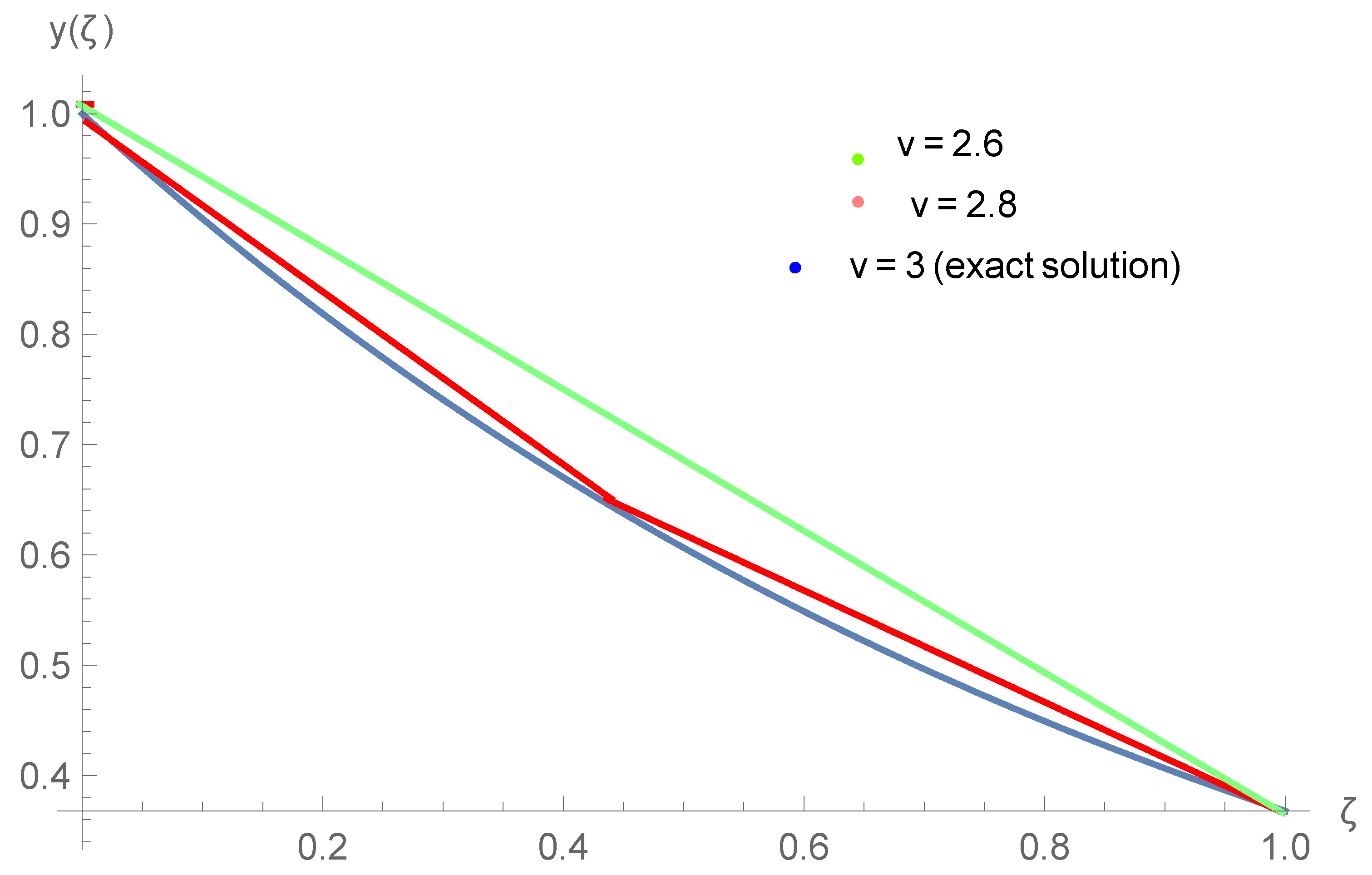
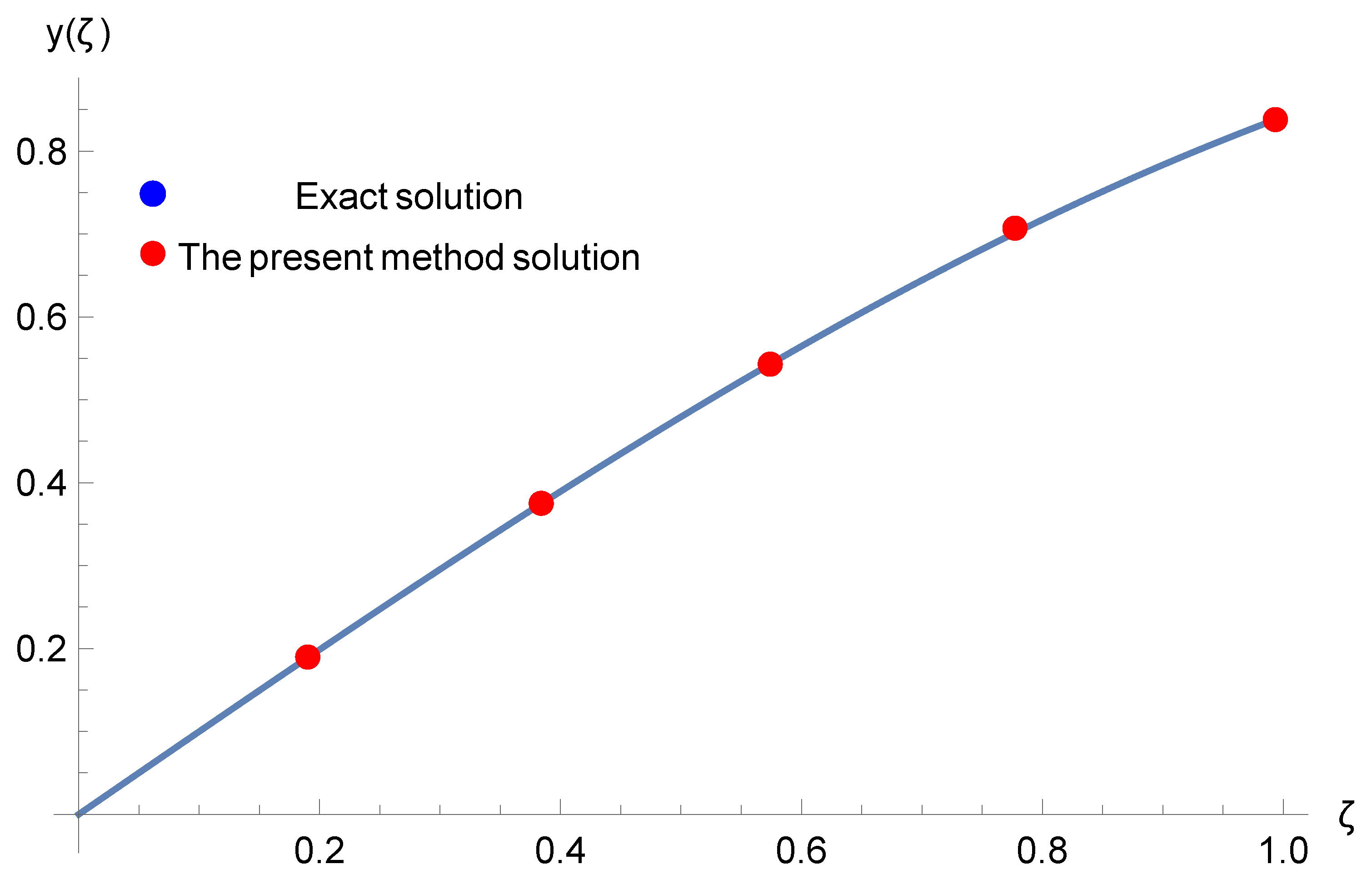
5. Illustrative Examples

This section considers five numerical examples to show the effectiveness of the proposed method for finding approximate solutions of the aforementioned fractional delay differential equations. The Mathematica 12 program is used to determine the numerical results.

Example 1.

Consider the linear FODDE:

$$\begin{array}{c}\hfill \begin{array}{cc}\hfill & D^v\left[\sigma -{\sigma }_0\right]\left(\zeta \right)=\alpha \sigma \left(\zeta \right)+\rho \left(\zeta \right)\left(\zeta \ge 0,\alpha <0\right),\hfill \\ \hfill & \sigma \left(0\right)={\sigma }_0,{\sigma }^{\prime }\left(0\right)={\sigma }_0^{\prime }.\hfill \end{array}\end{array}$$

(36)

If we choose $\rho \left(\zeta \right)={\zeta }^2+\frac{2}{\mathsf{\Gamma }\left(2.5\right)}{\zeta }^{2-v},v=0.5,\sigma \left(0\right)={\sigma }^{\prime }\left(0\right)=0$ and $\alpha =-1$, then (36) takes the form

$$\begin{array}{c}\hfill \begin{array}{cc}\hfill & D^{0.5}\sigma \left(\zeta \right)=-\sigma \left(\zeta \right)+{\zeta }^2+\frac{2}{\mathsf{\Gamma }\left(2.5\right)}{\zeta }^{1.5}\left(\zeta \ge 0,\alpha <0\right),\hfill \\ \hfill & \sigma \left(0\right)={\sigma }^{\prime }\left(0\right)=0,\hfill \end{array}\end{array}$$

(37)

and its exact solution is $\sigma \left(\zeta \right)={\zeta }^2$. The residual (32) takes the form

$$R\left(\zeta \right)=\left[{\chi }_{0.5}{H}_{0.5}{M}^T+\chi M^T+{\chi }_{-1}{H}_{-1}{M}^T\right]A-G.$$

(38)

Moreover, the initial conditions give the following two algebraic equations:

$$\begin{array}{cc}\hfill \sigma \left(0\right)& =\chi \left(0\right)M^{T}A=0,\hfill \end{array}$$

(39)

$$\begin{array}{cc}\hfill {\sigma }^{\prime }\left(0\right)& =\chi \left(0\right)B{M}^{T}A=0.\hfill \end{array}$$

(40)

By solving this algebraic equations, we obtain the coefficients vector as

$$A=\left(\begin{array}{ccccccc}\frac{1}{4}& 0& \frac{1}{4}& 0& 0& 0& 0\end{array}\right).$$

(41)

Then, by making use of the truncated Chebyshev series (20) with $N=6$, we obtain the solution of (37) as follows:

$$\begin{array}{cc}\hfill {\sigma }_6\left(\zeta \right)=\frac{1}{4}{\mathrm{Y}}_0\left(\zeta \right)+\left(0\right){\mathrm{Y}}_1\left(\zeta \right)+\frac{1}{4}{\mathrm{Y}}_2\left(\zeta \right)+& \left(0\right){\mathrm{Y}}_3\left(\zeta \right)\hfill \\ \hfill & +\left(0\right){\mathrm{Y}}_4\left(\zeta \right)+\left(0\right){\mathrm{Y}}_5\left(\zeta \right)+\left(0\right){\mathrm{Y}}_6\left(\zeta \right)={\zeta }^2.\hfill \end{array}$$

(42)

Thus, we obtain the same exact solution of Equation (37). While in [26], the exact solution could not be achieved, the numerical solution was achieved.

Example 2.

In this example, we consider the linear FODDE:

$$\begin{array}{c}\hfill \begin{array}{cc}\hfill & D^{\frac{1}{2}}\sigma \left(\zeta \right)+\sigma \left(\zeta \right)+\sigma (\zeta -1)=2\zeta +\frac{\mathsf{\Gamma }\left(3\right)}{\mathsf{\Gamma }\left(1.5\right)}{\zeta }^{1.5}-1,\hfill \\ \hfill & \sigma \left(0\right)=0,\hfill \end{array}\end{array}$$

(43)

The exact solution is $\sigma \left(\zeta \right)=4{\zeta }^2$.

Now, we apply our method to (43) at $\mu =5$. First, we have the following residual:

$$R\left(\zeta \right)=\left[{\chi }_{0.5}{H}_{0.5}{M}^T+\chi M^T-\chi B_{-1}{M}^T\right]A-G.$$

(44)

Additionally, the initial condition gives the following algebraic equation:

$$\sigma \left(0\right)=\chi \left(0\right)M^{T}A=0.$$

(45)

Solving this, it follows that

$$A=\left(\begin{array}{ccccccc}\frac{1}{2}& 1& \frac{1}{2}& 0& 0& 0& 0\end{array}\right).$$

(46)

Thus, the exact solution can be obtained by using (20) with $N=6$:

$${\sigma }_5\left(\zeta \right)=\frac{1}{2}{\mathrm{Y}}_0\left(\zeta \right)+\frac{1}{2}{\mathrm{Y}}_2\left(\zeta \right)=4{\zeta }^2.$$

(47)

It is important to be noticed in [28] that the solution is obtained by using the shifted Jacobi polynomial method.

Example 3.

Consider the following FODDE:

$$\begin{array}{c}\hfill \begin{array}{cc}\hfill & D^v\sigma \left(\zeta \right)+\sigma \left(\zeta \right)+\sigma (\zeta -0.3)=e^{-\zeta +0.3}\left(2<v\le 3\right),\hfill \\ \hfill & \sigma \left(0\right)=1,{\sigma }^{\prime }\left(0\right)=-1.\hfill \end{array}\end{array}$$

(48)

The exact solution of this equation is $\sigma \left(\zeta \right)=e^{-\zeta }$ for $v=3$. Here, we have the following residual:

$$R\left(\zeta \right)=\left[{\chi }_3{H}_3{M}^T+\chi M^T+\chi B_{-0.3}{M}^T\right]A-G.$$

(49)

The initial conditions lead to

$$\begin{array}{cc}\hfill \sigma \left(0\right)& =\chi \left(0\right)M^{T}A=1,\hfill \end{array}$$

(50)

$$\begin{array}{cc}\hfill {\sigma }^{\prime }\left(0\right)& =\chi \left(0\right)B{M}^{T}A=-1,\hfill \end{array}$$

(51)

and we can solve these equations with $v=3$ to get

$$A=\left(\begin{array}{ccccc}1.26604-1.12997& 0.27146-0.04426& 0.00546& 0.00546-0.00056& 0.00004\end{array}\right).$$

(52)

Table 1. Comparison results for Example 3.

$\mathit{\zeta }$	Exact	Present Method	[39] $\mathit{\mu }=7$	[38] $\mathit{\mu }=7$	Presented Method	Presented Method
	Solution	($\mathit{\mu }=6$) ($\mathit{v}=3$)	$\mathit{v}=3$	$\mathit{v}=3$	($\mathit{\mu }=6$) $\mathit{v}=2.8$	($\mathit{\mu }=6$) ($\mathit{v}=2.6$)
0	1.00000	1.00000	1.0000	1.0000	1.0000	1.0000
0.2	0.8187	0.8187	0.8187	0.8187	0.8185	0.8185
0.4	0.6703	0.6703	0.6703	0.6703	0.6685	0.6682
0.6	0.5488	0.5488	0.5488	0.5488	0.5480	0.5488
0.8	0.4493	0.4493	0.4494	0.4493	0.4366	0.4281
1	0.3679	0.3679	0.3679	0.3680	0.3679	0.3652

demonstrates the comparison of the exact solution with our present method calculated for $\mu =6$, the Hermite wavelet method presented in [38] calculated for $\mu =7$ and the Bernoulli wavelet method presented in [39]. Additionally, the numerical results for (48) at $v=2.8$ and $2.6$ are involved in the same table. In addition, Figure 1 demonstrates the numerical solutions at different values of v and the exact solution $(v=3)$. As the table and figure suggest, the current method produces smaller absolute errors.

Example 4.

We consider the FODDE:

$$\begin{array}{c}\hfill \begin{array}{cc}\hfill & D^{\frac{3}{10}}\sigma \left(\zeta \right)-\sigma (\zeta -1)+\sigma \left(\zeta \right)=1-3\zeta +3{\zeta }^2+\frac{2000{\zeta }^{2.7}}{1071\mathsf{\Gamma }\left(1.7\right)},\hfill \\ \hfill & \sigma \left(0\right)=0.\hfill \end{array}\end{array}$$

(53)

The exact solution for this equation is $\sigma \left(\zeta \right)=2{\zeta }^3+\frac{5}{3}\zeta$.

The fundamental matrix equation for this problem is given by

$$R\left(\zeta \right)=\left[{\chi }_{\frac{3}{10}}{H}_{\frac{3}{10}}{M}^T+\chi M^T+\chi B_{-1}{M}^T\right]A-G,$$

(54)

and the coefficient matrix can be obtained after the augmented matrices of the system and the initial condition are computed as follows:

$$A=\left(\begin{array}{ccccccc}0& \frac{3}{4}& 0& \frac{1}{4}& 0& 0& 0\end{array}\right).$$

(55)

Therefore, according to (20) with $\mu =6$, the solution of (53) is given by

$${\sigma }_6\left(\zeta \right)=\frac{3}{4}{\mathrm{Y}}_1\left(\zeta \right)+\frac{1}{4}{\mathrm{Y}}_3\left(\zeta \right)=2{\zeta }^3+\frac{5}{3}\zeta ,$$

(56)

and this is the exact solution of (53). Again, the numerical solution follows the exact solution exactly.

Example 5.

In our last example, we consider the FODDE:

$$\begin{array}{c}\hfill \begin{array}{cc}\hfill & D^2\sigma \left(\zeta \right)-\frac{1}{2}{\sigma }^{\prime }(\zeta -\pi )+\frac{1}{2}\sigma \left(\zeta \right)=0,\hfill \\ \hfill & \sigma \left(0\right)=0,{\sigma }^{\prime }\left(0\right)=1.\hfill \end{array}\end{array}$$

(57)

Its exact solution is given by $\sigma \left(\zeta \right)=sin\left(\zeta \right)$.

The following residual can be obtained for $\mu =6$:

$$R\left(\zeta \right)=\left[{\chi }_2{H}_2{M}^T+Q_1\chi H{B}_{-\pi }{M}^T+Q_0\chi M^T\right]A.$$

(58)

The initial condition also leads to

$$\begin{array}{cc}\hfill \sigma \left(0\right)& =\chi \left(0\right)M^{T}A=0,\hfill \end{array}$$

(59)

$$\begin{array}{cc}\hfill {\sigma }^{\prime }\left(0\right)& =\chi \left(0\right)B{M}^{T}A=1.\hfill \end{array}$$

(60)

Solving this system with $v=2$, we have

$$A=\left(\begin{array}{ccccccc}0& 0.880196& 0& -0.039119& 0& 0.000488& 0\end{array}\right).$$

(61)

Then, the solution of (54) is as follows:

$${\sigma }_6\left(\zeta \right)=0.880196{\mathrm{Y}}_1\left(\zeta \right)-0.039119{\mathrm{Y}}_3\left(\zeta \right)+0.000488{\mathrm{Y}}_5\left(\zeta \right).$$

(62)

The results are summarized in

Table 2. Comparison of the present method with the exact solution for Example 5.

$\mathit{\zeta }$	Exact	Present Method
	Solution	($\mathit{\mu }=6$), $\mathit{\nu }=2$
0.2	0.1975	0.1985
0.4	0.3894	0.3892
0.6	0.5646	0.5645
0.8	0.7173	0.7173
1	0.8414	0.8414

and Figure 2. They show the comparison of solutions between the present method and the exact solution for $\mu =6,v=2$ and $\zeta \in [0,1]$.

6. Conclusions

Considerable attention is paid to fractional-order differential equations because they appear to be more effective for modeling and analyzing dynamical processes in basic and engineering and sciences. For this reason, finding and successfully applying new approaches and methods for solving these equations happens to have been one of the essential concerns for mathematical and applied scientists for many decades.

In our current work, we aimed to present the general form of FODDEs with the linear functional argument. Additionally, the exact as well as numerical solutions of these FODDEs were the utmost priority by using the spectral Tau method. Furthermore, the main matrix transformation technique, which we used in our investigation, is a linear fractional argument based on the method involving the method of generalized Chebyshev polynomials of the second kind. This was indeed proved as one of the most efficient methodologies for reducing all terms in the proposed FODDE. Due mainly to the high volume of symbolic calculations in the proposed method, it became necessary to use such symbolic software packages as Mathematica 12 in completing the required steps of the above procedures. In order to investigate the efficiency and accuracy of the methodology used here, five numerical FODDE examples and two figures were given in the article. We also explained the comparisons of the method, which we used here, with the other existing methods.

On the basis of results presented in this article, it is concluded that the method, which we proposed and applied here, is a more convenient and effective technique than the other existing techniques, and it can be used in solving FODDEs in the fields of engineering and science. This suggests that the spectral Tau method has the potential to be applied to solve other nonlinear FODDE models.

References

1. Vanani, S.K.; Aminataei, A. Tau approximate solution of fractional partial differential equations. Comput. Math. Appl. 2011, 62, 1075–1083. [Google Scholar] [CrossRef] [Green Version]
2. Ghoreishi, F.; Yazdani, S. An extension of the spectral Tau method for numerical solution of multi-order fractional differential equations with convergence analysis. Comput. Math. Appl. 2011, 61, 30–43. [Google Scholar] [CrossRef] [Green Version]
3. Ren, R.-F.; Li, H.-B.; Jiang, W.; Song, M.-Y. An efficient Chebyshev-Tau method for solving the space fractional diffusion equations. Appl. Math. Comput. 2013, 224, 259–267. [Google Scholar] [CrossRef]
4. Eslahchi, M.R.; Dehghan, M.; Parvizi, M. Application of the collocation method for solving nonlinear fractional integro-differential equations. J. Comput. Appl. Math. 2014, 257, 105–128. [Google Scholar] [CrossRef]
5. Tohidi, E.; Bhrawy, A.H.; Erfani, K. A collocation method based on Bernoulli operational matrix for numerical solution of generalized pantograph equation. Appl. Math. Model. 2013, 37, 4283–4294. [Google Scholar] [CrossRef]
6. Sedaghat, S.; Ordokhani, Y.; Dehghan, M. Numerical solution of the delay differential equations of pantograph type via Chebyshev polynomials. Commun. Nonlinear Sci. Numer. Simul. 2012, 17, 4815–4830. [Google Scholar] [CrossRef]
7. Izadi, M.; Srivastava, H.M. A novel matrix technique for multi-order pantograph differential equations of fractional order. Proc. R. Soc. Lond. Ser. A 2021, 477, 2021031. [Google Scholar] [CrossRef]
8. Hafshejani, M.S.; Vanani, S.K.; Hafshejani, J.S. Numerical solution of delay differential equations using Legendre wavelet method. World Appl. Sci. J. 2011, 13, 27–33. [Google Scholar]
9. Marzban, H.R.; Razzaghi, M. Solution of multi-delay systems using hybrid of block-pulse functions and Taylor series. J. Sound Vib. 2006, 292, 954–963. [Google Scholar] [CrossRef]
10. Tang, X.; Shi, Y.; Xu, H. Well conditioned pseudospectral schemes with tunable basis for fractional delay differential equations. J. Sci. Comput. 2018, 74, 920–936. [Google Scholar] [CrossRef]
11. Khader, M.M.; Hendy, A.S. The approximate and exact solutions of the fractional-order delay differential equations using Legendre pseudospectral method. Int. J. Pure Appl. Math. 2012, 74, 287–297. [Google Scholar]
12. Wang, Z. A numerical method for delayed fractional-order differential equations. J. Appl. Math. 2013, 2013, 256071. [Google Scholar] [CrossRef]
13. Moghaddam, B.P.; Mostaghim, Z.S. A numerical method based on finite difference for solving fractional delay differential equations. J. Taibah Univ. Sci. 2013, 7, 120–127. [Google Scholar] [CrossRef] [Green Version]
14. Li, Y.-L.; Zhao, W.-W. Haar wavelet operational matrix of fractional order integration and its applications in solving the fractional order differential equations. Appl. Math. Comput. 2010, 216, 2276–2285. [Google Scholar] [CrossRef]
15. Iqbal, M.A.; Ali, A.; Mohyud-Din, S.T. Chebyshev wavelets method for fractional delay differential equations. Int. J. Mod. Appl. Phys. 2013, 4, 49–61. [Google Scholar]
16. Keshavarz, E.; Ordokhani, Y.; Razzaghi, M. Bernoulli wavelet operational matrix of fractional order integration and its applications in solving the fractional order differential equations. Appl. Math. Model. 2014, 38, 6038–6051. [Google Scholar] [CrossRef]
17. Dehghan, M.; Manafian, J.; Saadatmandi, A. Solving nonlinear fractional partial differential equations using the homotopy analysis method. Numer. Methods Partial Differ. Equ. 2010, 26, 448–479. [Google Scholar] [CrossRef]
18. Saadatmandi, A.; Dehghan, M. A Tau approach for solution of the space fractional diffusion equation. Comput. Math. Appl. 2011, 62, 1135–1142. [Google Scholar] [CrossRef] [Green Version]
19. Azizi, M.R.; Saadatmandi, A.; Dehghan, M. The Sinc Legendre collocation method for a class of fractional convection diffusion equations with variable coefficients. Commun. Nonlinear Sci. Numer. Simul. 2012, 17, 4125–4136. [Google Scholar]
20. Manafian, J.; Dehghan, M.; Saadatmandi, A. The solution of the linear fractional partial differential equations using the homotopy analysis method. Z. Naturforsh. A 2010, 65, 935. [Google Scholar]
21. Iakovleva, V.; Vanegas, C.J. On the solution of differential equations with delayed and advanced arguments. Electron. J. Differ. Equ. Conf. 2005, 13, 57–63. [Google Scholar]
22. Rus, A.I.; Dârzu-Ilea, V.A. First order functional-differential equations with both advanced and retarded arguments. Fixed Point Theory 2004, 5, 103–115. [Google Scholar]
23. Mohammed, P.O.; Machado, J.A.T.; Guirao, J.L.G.; Agarwal, R.P. Adomian decomposition and fractional power series solution of a class of nonlinear fractional differential equations. Mathematics 2021, 9, 1070. [Google Scholar] [CrossRef]
24. Sana, G.; Mohammed, P.O.; Shin, D.Y.; Noor, M.A.; Oudat, M.S. On iterative methods for solving nonlinear equations in quantum calculus. Fractal Fract. 2021, 5, 60. [Google Scholar] [CrossRef]
25. Grbz, F.; Ding, S.; Han, H.; Long, P. A characterization of rough fractional type integral operators and Campanato estimates for their commutators on the variable exponent vanishing generalized Morrey spaces. arXiv 2018, arXiv:1811.06702. [Google Scholar]
26. Reutskiy, S.Y. The backward substitution method for multipoint problems with linear Volterra-Fredholm integro-differential equations of the neutral type. J. Comput. Appl. Math. 2016, 296, 724–738. [Google Scholar] [CrossRef]
27. Ramadan, M.A.; Raslan, K.R.; El-Danaf, T.S.; Abd-El-Salam, M.A. An exponential Chebyshev second kind approximation for solving high-order ordinary differential equations in unbounded domains, with application to Dawson’s integral. J. Egypt. Math. Soc. 2017, 25, 197–205. [Google Scholar] [CrossRef] [Green Version]
28. Raslan, K.R.; Khalid, K.A.; Emad, M. Spectral Tau method for solving general fractional order differential equation with linear functional argument. J. Egypt. Math. Soc. 2019, 27, 1–16. [Google Scholar] [CrossRef] [Green Version]
29. Lazarević, M.P.; Rapaić, M.R.; Šekara, T.B. Introduction to Fractional Calculus with Brief Historical Background. In Advanced Topics on Applications of Fractional Calculus on Control Problems, System Stability and Modelin; Mladenov, V., Mastorakis, N., Eds.; WSEAS Press: New York, NY, USA, 2014; pp. 3–16. [Google Scholar]
30. Mohammed, P.O.; Abdeljawad, T.; Hamasalh, F.K. On Discrete delta Caputo-Fabrizio fractional operators and monotonicity analysis. Fractal Fract. 2021, 5, 116. [Google Scholar] [CrossRef]
31. Diethelm, K. The Analysis of Fractional Differential Equations; Springer: Berlin/Heidelberg, Germany, 2010. [Google Scholar]
32. Molliq, R.Y.; Noorani, M.S.M.; Hashim, I. Variational iteration method for fractional heat- and wave-like equations. Nonlinear Anal. Real World Appl. 2009, 10, 1854–1869. [Google Scholar] [CrossRef]
33. Kilbas, A.A.; Srivastava, H.M.; Trujillo, J.J. Theory and Applications of Fractional Differential Equations; North-Holland Mathematics Studies; Elsevier: Amsterdam, The Netherlands, 2006; Volume 204. [Google Scholar]
34. Baleanu, D.; Fernandez, A. On fractional operators and their classifications. Mathematics 2019, 7, 830. [Google Scholar] [CrossRef] [Green Version]
35. Srivastava, H.M. Fractional-order derivatives and integrals: Introductory overview and recent developments. Kyungpook Math. J. 2020, 60, 73–116. [Google Scholar]
36. Srivastava, H.M. Some parametric and argument variations of the operators of fractional calculus and related special functions and integral transformations. J. Nonlinear Convex Anal. 2021, 22, 1501–1520. [Google Scholar]
37. Srivastava, H.M. An introductory overview of fractional-calculus operators based upon the Fox-Wright and related higher transcendental functions. J. Adv. Eng. Comput. 2021, 5, 135–166. [Google Scholar]
38. Saeed, U. Hermite wavelet method for fractional delay differential equations. J. Differ. Equ. 2014, 2014, 1–8. [Google Scholar] [CrossRef] [Green Version]
39. Rahimkhani, P.; Ordokhani, Y.; Babolian, E. A new operational matrix based on Bernoulli wavelets for solving fractional delay differential equations. Numer. Algorithms 2017, 74, 223–245. [Google Scholar] [CrossRef]
Figure 1. Numerical and exact solutions at different values of α and μ = 6 for Example 3.
Fractalfract 06 00007 g001
Figure 2. Exact and approximate solutions for μ = 6 , v = 2 and ζ [ 0 , 1 ] , for Example 5.
Fractalfract 06 00007 g002