
The Role of the Discount Policy of Prepayment on Environmentally Friendly Inventory Management

 ,
,  ,
,  , , and
Abstract
:1. Introduction
- How do payment-in-advance models affect pricing and replenishment decisions as well as the total profit when customer demand is sensitive to the selling price and environmental performance of the producer?
- Will discount policy impact retailers’ choice of payment in advance settings and total profit?
- How do the customer preference for carbon emission reduction levels and various emission costs impact the retailer’s total profit?
2. Literature Review
3. Mathematical Model Formulation for Inventory Model
- Inventory of a single product is considered with a limitless planning horizon.
- The replenishment rate is boundless.
- The lead time is constant and the shortages are overlooked.
- The retailer has to make a payment in advance to the supplier [23].
- The supplier offers a discount on the purchase cost of the products according to the number of instalment decisions [23].
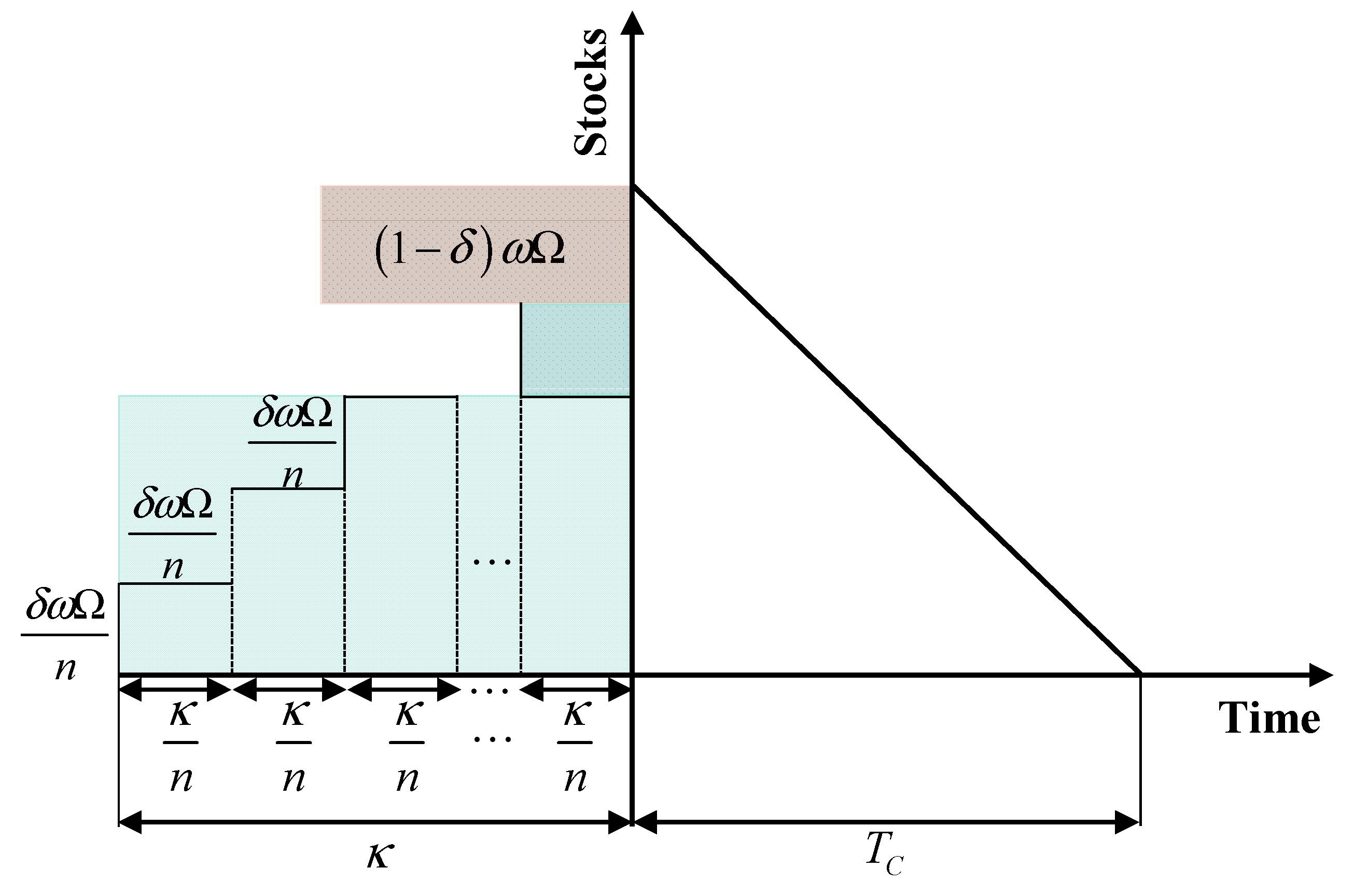
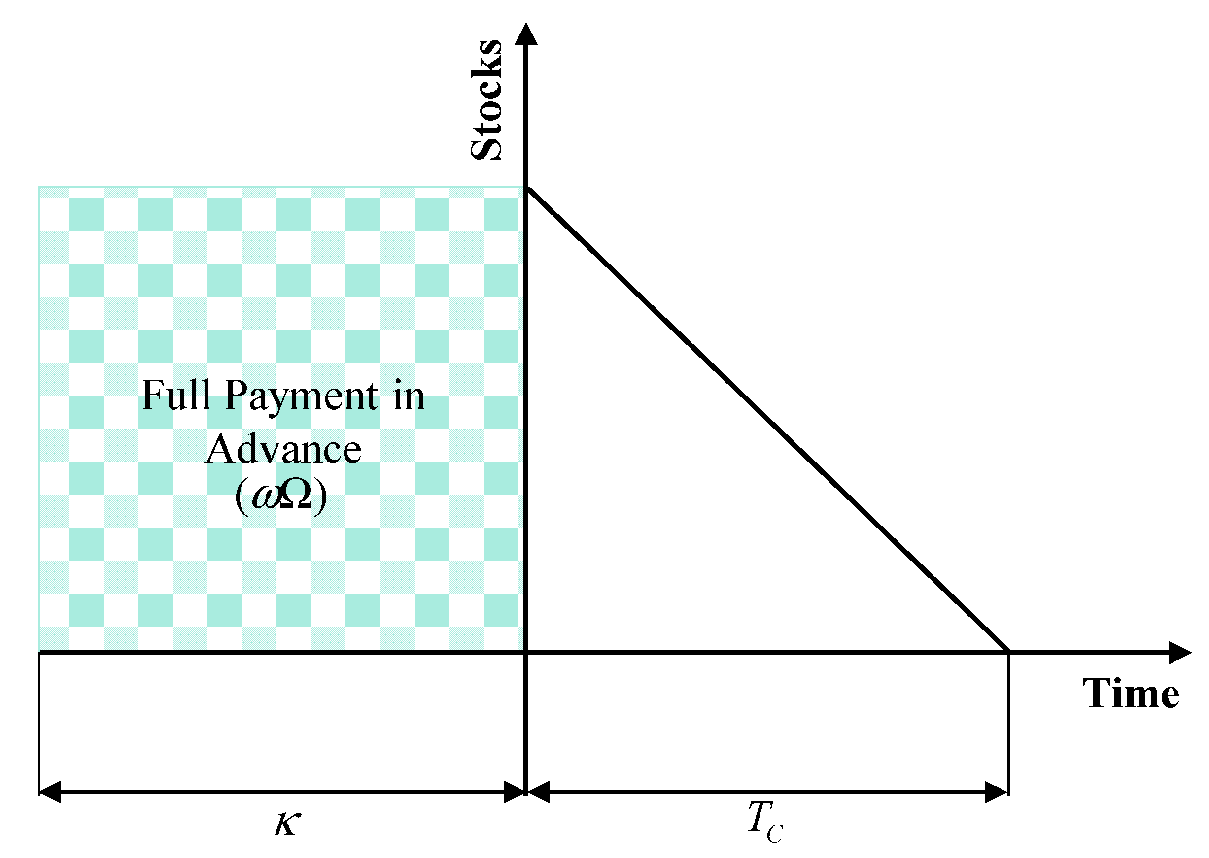
3.1. Case I: With Advanced Payment and a Discount for Instalment Based Payment
3.1.1. Total Cost per Unit Time
- (a)
- Ordering cost per cycle:
- (b)
- The inventory holding cost per cycle:
- (c)
- The purchase cost per cycle:
- (d)
- Transportation cost per cycle:
- (e)
- Instalment capital cost:
- (f)
- Discount on purchase cost:
- (g)
- Carbon emission reduction cost:
- (h)
- Sales revenue per cycle:
3.1.2. Total Profit per Unit Time
3.2. Case II: With Advanced Payment and a Discount for Single Time Payment
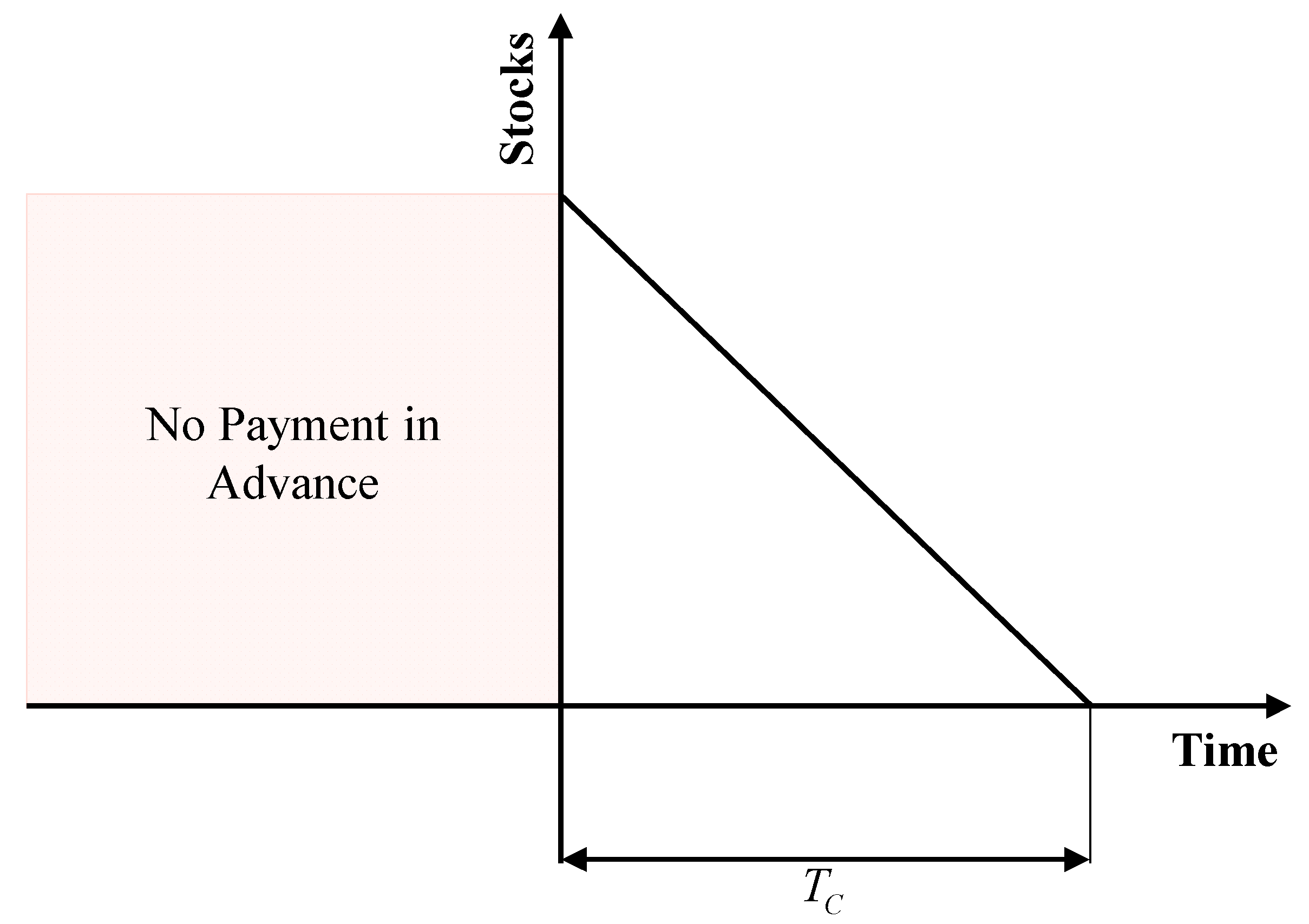
3.3. Case III: Without Advanced Payment
4. Theoretical Development
4.1. Case I (with Advanced Payment and a Discount for Instalment Based Payment)
4.2. Case II: With Advanced Payment and a Discount for Single Time Payment
4.3. Case III: Without Advanced Payment
5. Analysis and Discussion
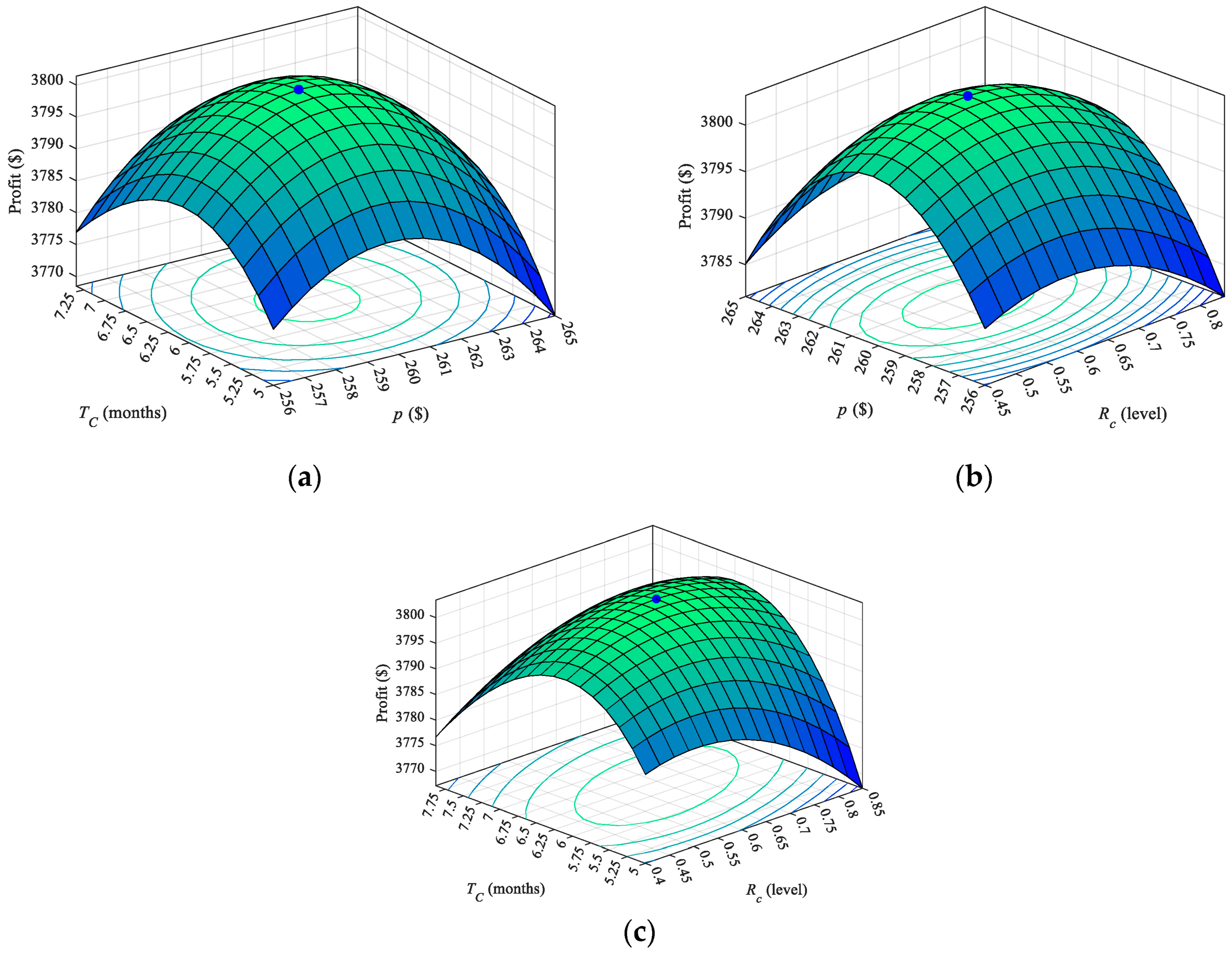
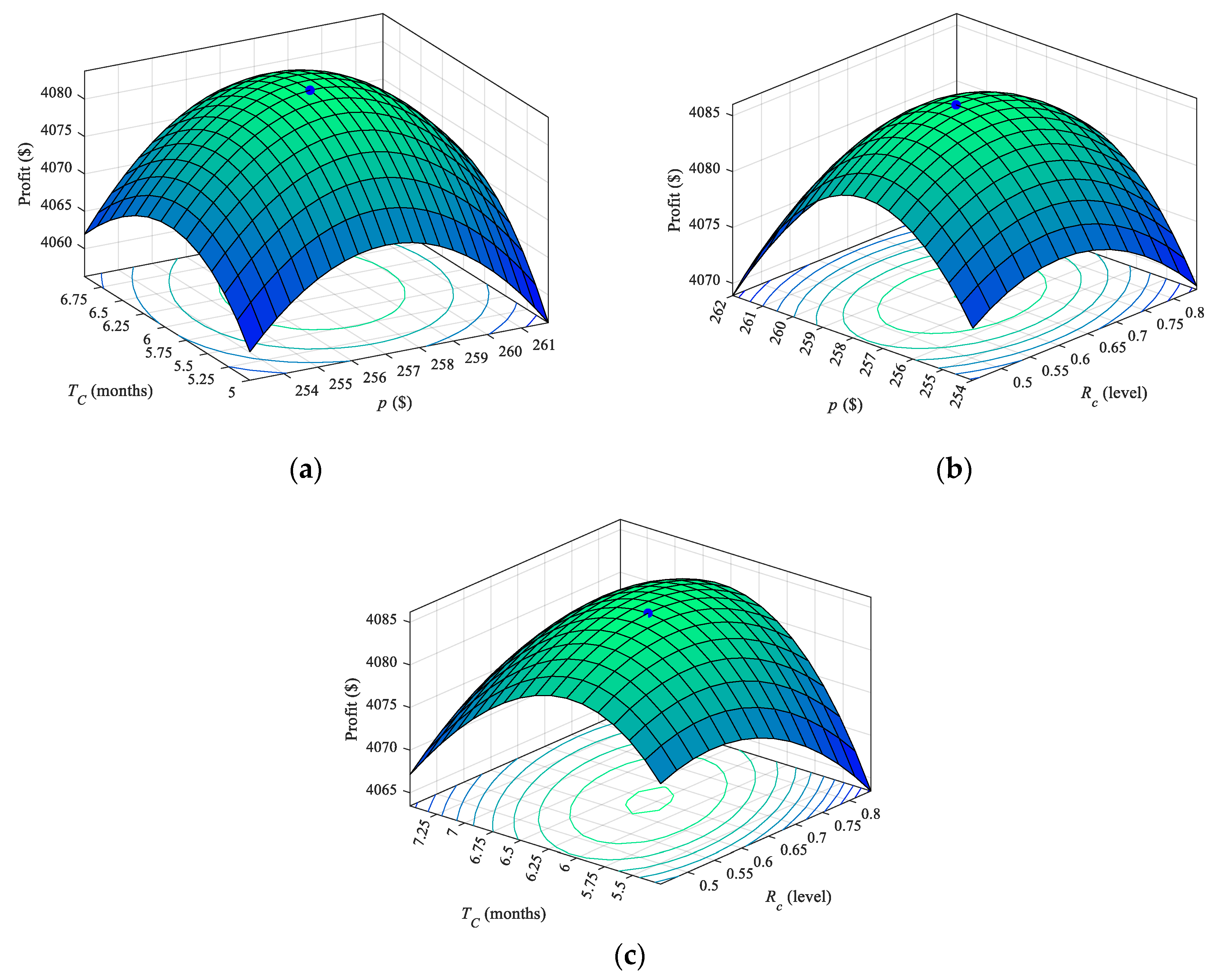
5.1. Case Study
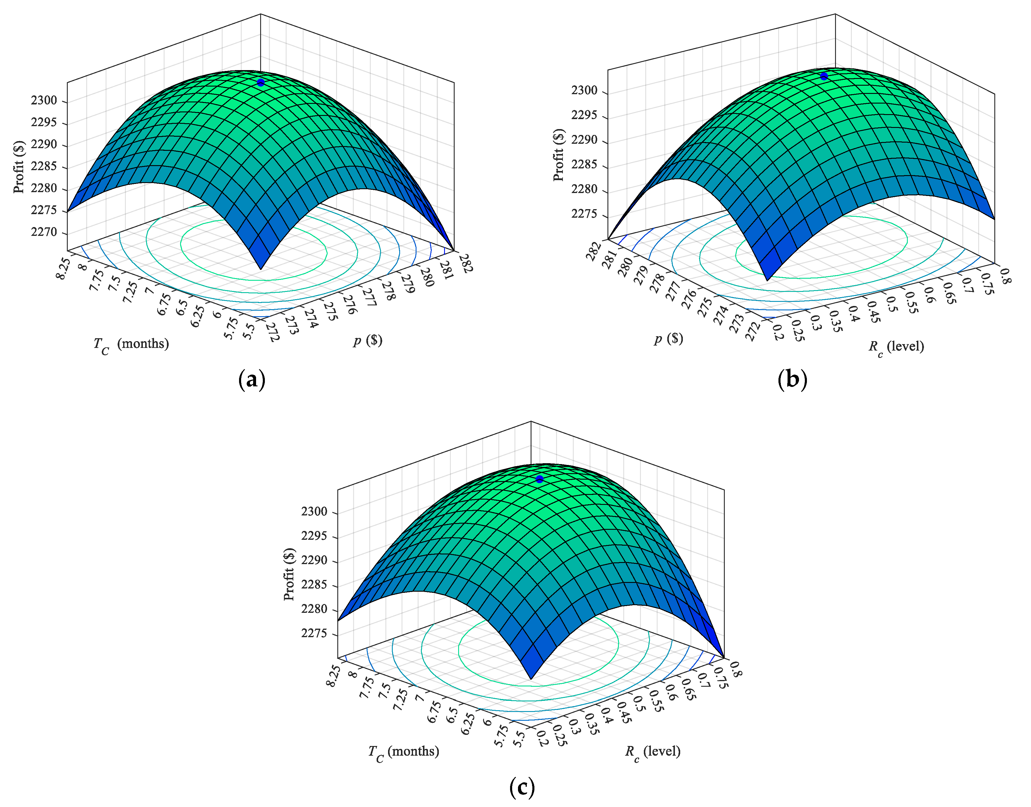
5.2. Numerical Illustration
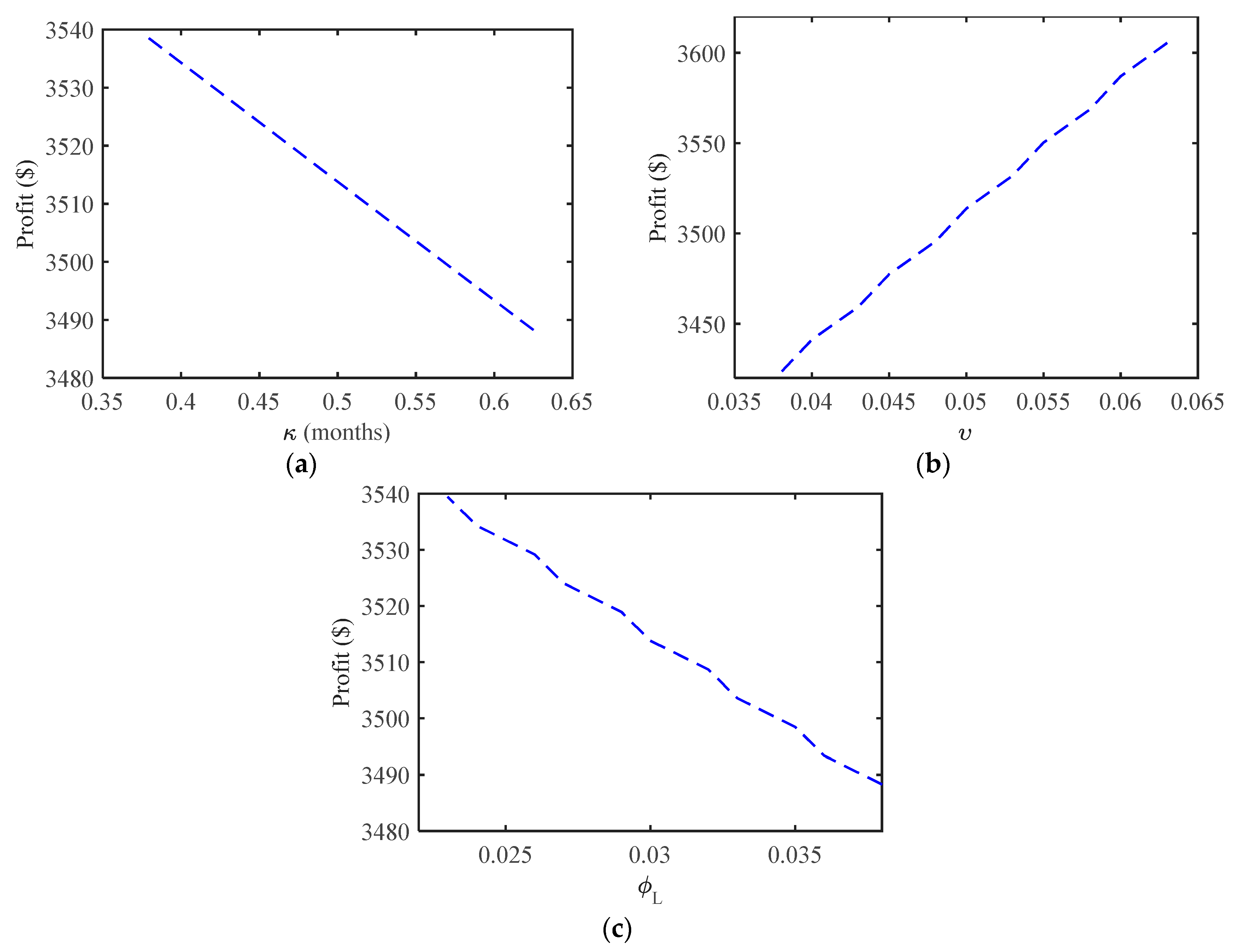
5.3. Sensitivity Analysis
- The market potential is positively correlated with the integrated profit. The selling price is correlated similarly, but the cycle length interacts negatively. One can detect the continuous rise in profit and selling price with growing market potential for all these three cases, and the profit becomes maximum for Case II, whereas the selling price, as well as cycle length, become minimum.
- The total profit and selling price decline for all three cases as the price elasticity parameter increases. The cycle length behaves in the opposite direction. One can observe the highest profit at the minimum value of the price elasticity parameter for a discount on a single-instalment payment (Case II).
- The total profit increases for all three cases with higher values of carbon emission reduction level (). The selling price and the cycle length show the same characteristics. The total profit is comparatively much lower in Case I as the instalment policy creates an extra cost. The profit is best in Case II, since the discount in purchasing cost influences higher profit gaining.
- For all three cases, the ordering cost , as well as the holding cost , have a direct impact on total profit. The higher values of those two costs create a lower profit and vice versa. The increasing ordering charge or holding charge means a decline in profit. It is easy to observe the significant consequence of this fact for all three cases. A similar type of effect has been noted for fluctuations of the per-unit purchase cost .
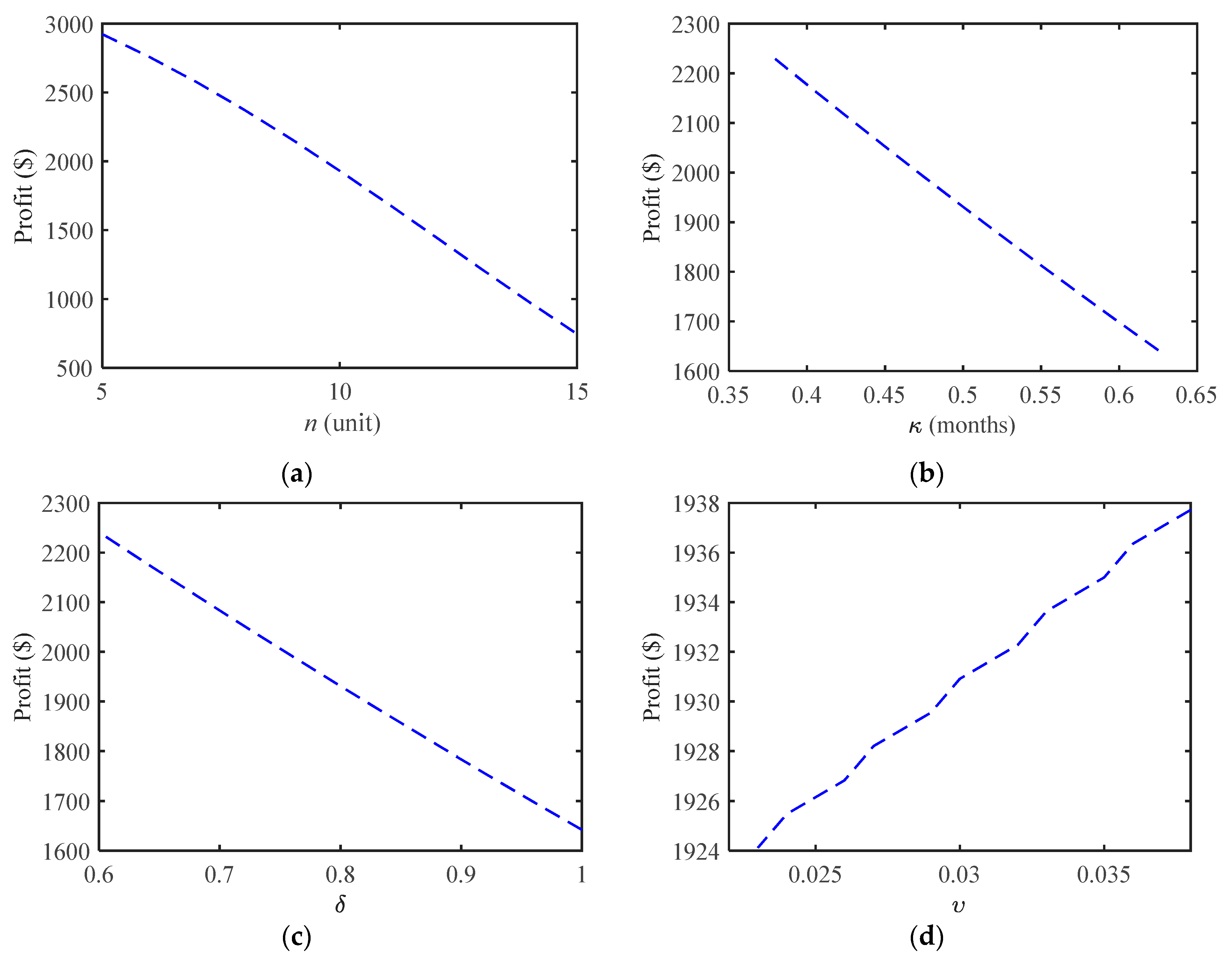
- The larger the number of trips the lesser the profit becomes since an extra trip means it needs an additional fixed cost, variable cost, fuel, labor, etc. Therefore, the profit becomes lower for the intensifications of trips. The travel distance , fuel cost , fuel consumption per ton of payload (), and product weight () have similar impacts on profit as those can add additional expenses. Any longer distance brings additional cost in the expenses, so reduction of distance can optimize the profit, which is numerically true, as shown in the sensitivity table.
- The implications of carbon emission cost on transportation cost have important roles in profit gaining. Increasing values of carbon emission cost per unit distance () and carbon emission cost per unit item per unit distance () force the total profit to be less in all three cases.
5.4. Managerial Implications
- (i)
- From the three observed cases, the lowest selling price is obtained when the payment in advance is performed in a single payment. Further study also confirms that profit is higher for a smaller number of instalments; hence, managers can optimize the number of installments in this direction considering their financial condition.
- (ii)
- The case with a single payment also results in a lower selling price. It is beneficial for customers and increases the demand level.
- (iii)
- One can take important pricing decisions from the study and maintain a healthy profit margin by incorporating these strategies and simultaneously observing the nature of the customers.
- (iv)
- This study provides some insights into how preferences for low carbon can influence the sales of the retailer and in which way a manager can maintain an eco-friendly inventory. This study shows that the total profit increases with higher values of carbon emission reduction level and higher preferences for low carbon among customers.
6. Conclusions
- (i)
- The optimal replenishment rate clinging to the commencement of payment in advance has been successfully integrated and offers some significant results.
- (ii)
- Simultaneous integration of discount policy, payment in advance to the selling price, and reduction of carbon-emission-dependent demand work efficiently. It provides some techniques for the retailer to manage inventories profitably.
- (iii)
- A smaller number of instalments of the payment in advance increase the profit. This study shows that the case with a single payment results in a higher total profit and a lower selling price.
- (iv)
- With the increasing customers’ preferences for environmentally friendly products, retailers should increase the effort for reducing emission levels.
Author Contributions
Funding
Institutional Review Board Statement
Informed Consent Statement
Data Availability Statement
Acknowledgments
Conflicts of Interest
References
- Borin, N.; Lindsey-Mullikin, J.; Krishnan, R. An analysis of consumer reactions to green strategies. J. Prod. Brand Manag. 2013, 22, 118–128. [Google Scholar] [CrossRef]
- Lin, R.-J.; Tan, K.-H.; Geng, Y. Market demand, green product innovation, and firm performance: Evidence from Vietnam motorcycle industry. J. Clean. Prod. 2013, 40, 101–107. [Google Scholar] [CrossRef]
- Zhang, Q.; Zhao, Q.; Zhao, X.; Tang, L. On the introduction of green product to a market with environmentally conscious consumers. Comput. Ind. Eng. 2020, 139, 106190. [Google Scholar] [CrossRef]
- Fernando, Y.; Wah, W.X. The impact of eco-innovation drivers on environmental performance: Empirical results from the green technology sector in Malaysia. Sustain. Prod. Consum. 2017, 12, 27–43. [Google Scholar] [CrossRef]
- Yalabik, B.; Fairchild, R.J. Customer, regulatory, and competitive pressure as drivers of environmental innovation. Int. J. Prod. Econ. 2011, 131, 519–527. [Google Scholar] [CrossRef]
- Pang, Q.; Li, M.; Yang, T.; Shen, Y. Supply chain coordination with carbon trading price and consumers’ environmental awareness dependent demand. Math. Probl. Eng. 2018, 2018, 8749251. [Google Scholar] [CrossRef] [Green Version]
- Xia, L.; Hao, W.; Qin, J.; Ji, F.; Yue, X. Carbon emission reduction and promotion policies considering social preferences and consumers’ low-carbon awareness in the cap-and-trade system. J. Clean. Prod. 2018, 195, 1105–1124. [Google Scholar] [CrossRef]
- Xia, L.; Guo, T.; Qin, J.; Yue, X.; Zhu, N. Carbon emission reduction and pricing policies of a supply chain considering reciprocal preferences in cap-and-trade system. Ann. Oper. Res. 2017, 268, 149–175. [Google Scholar] [CrossRef]
- Zanoni, S.; Mazzoldi, L.; Zavanella, L.E.; Jaber, M.Y. A joint economic lot size model with price and environmentally sensitive demand. Prod. Manuf. Res. 2014, 2, 341–354. [Google Scholar] [CrossRef] [Green Version]
- Sana, S.S. A structural mathematical model on two echelon supply chain system. Ann. Oper. Res. 2021. [Google Scholar] [CrossRef]
- Hovelaque, V.; Bironneau, L. The carbon-constrained EOQ model with carbon emission dependent demand. Int. J. Prod. Econ. 2015, 164, 285–291. [Google Scholar] [CrossRef]
- Tsai, P.-H.; Lin, G.-Y.; Zheng, Y.-L.; Chen, Y.-C.; Chen, P.-Z.; Su, Z.-C. Exploring the effect of Starbucks’ green marketing on consumers’ purchase decisions from consumers’ perspective. J. Retail. Consum. Serv. 2020, 56, 102162. [Google Scholar] [CrossRef]
- Nekmahmud, M.; Fekete-Farkas, M. Why not green marketing? Determinates of consumers’ intention to green purchase decision in a new developing nation. Sustainability 2020, 12, 7880. [Google Scholar] [CrossRef]
- Grant, J. Green marketing. Strateg. Dir. 2008, 24, 25–27. [Google Scholar] [CrossRef]
- Ginsberg, J.; Bloom, P. Choosing the right green marketing strategy. MIT Sloan Manag. Rev. 2004, 79–84. [Google Scholar]
- Lampe, M.; Gazda, G.M. Green marketing in Europe and the United States: An evolving business and society interface. Int. Bus. Rev. 1995, 4, 295–312. [Google Scholar] [CrossRef]
- Dong, G.; Liang, L.; Wei, L.; Xie, J.; Yang, G. Optimization model of trade credit and asset-based securitization financing in carbon emission reduction supply chain. Ann. Oper. Res. 2021, 299, 1–50. [Google Scholar] [CrossRef]
- Zhang, Q.; Tsao, Y.-C.; Chen, T.-H. Economic order quantity under advance payment. Appl. Math. Model. 2014, 38, 5910–5921. [Google Scholar] [CrossRef]
- Taleizadeh, A.A.; Tavakoli, S.; San-José, L.A. A lot sizing model with advance payment and planned backordering. Ann. Oper. Res. 2018, 271, 1001–1022. [Google Scholar] [CrossRef]
- Li, R.; Skouri, K.; Teng, J.-T.; Yang, W.-G. Seller’s optimal replenishment policy and payment term among advance, cash, and credit payments. Int. J. Prod. Econ. 2018, 197, 35–42. [Google Scholar] [CrossRef]
- Maiti, A.K.; Maiti, M.K.; Maiti, M. Inventory model with stochastic lead-time and price dependent demand incorporating advance payment. Appl. Math. Model. 2009, 33, 2433–2443. [Google Scholar] [CrossRef]
- Taleizadeh, A.A. An economic order quantity model for deteriorating item in a purchasing system with multiple prepayments. Appl. Math. Model. 2014, 38, 5357–5366. [Google Scholar] [CrossRef]
- Mashud, A.H.M.; Roy, D.; Daryanto, Y.; Chakrabortty, R.K.; Tseng, M.-L. A sustainable inventory model with controllable carbon emissions, deterioration and advance payments. J. Clean. Prod. 2021, 296, 126608. [Google Scholar] [CrossRef]
- Sepehri, A. Inventory management under carbon emission policies: A systematic literature review. Decis. Mak. Invent. Manag. 2021, 187–218. [Google Scholar] [CrossRef]
- Pattnaik, S.; Nayak, M.M.; Abbate, S.; Centobelli, P. Recent trends in sustainable inventory models: A literature review. Sustainability 2021, 13, 11756. [Google Scholar] [CrossRef]
- Lin, T.-Y.; Sarker, B.R. A pull system inventory model with carbon tax policies and imperfect quality items. Appl. Math. Model. 2017, 50, 450–462. [Google Scholar] [CrossRef]
- Kazemi, N.; Abdul-Rashid, S.H.; Ghazilla, R.A.R.; Shekarian, E.; Zanoni, S. Economic order quantity models for items with imperfect quality and emission considerations. Int. J. Syst. Sci. Oper. Logist. 2016, 5, 99–115. [Google Scholar] [CrossRef]
- Shen, Y.J.; Shen, K.F.; Yang, C.T. A production inventory model for deteriorating items with collaborative preservation technology investment under carbon tax. Sustainability 2019, 11, 5027. [Google Scholar] [CrossRef] [Green Version]
- Wee, H.-M.; Daryanto, Y. Imperfect quality item inventory models considering carbon emissions. Optim. Invent. Manag. Asset 2020, 137–159. [Google Scholar] [CrossRef]
- Daryanto, Y.; Wee, H.M.; Wu, K.H. Revisiting sustainable EOQ model considering carbon emission. Int. J. Manuf. Technol. Manag. 2021, 35. [Google Scholar] [CrossRef]
- Paul, A.; Pervin, M.; Roy, S.K.; Maculan, N.; Weber, G.-W. A green inventory model with the effect of carbon taxation. Ann. Oper. Res. 2021. [Google Scholar] [CrossRef]
- As’ad, R.; Hariga, M.; Shamayleh, A. Sustainable dynamic lot sizing models for cold products under carbon cap policy. Comput. Ind. Eng. 2020, 149, 106800. [Google Scholar] [CrossRef] [PubMed]
- Hasan, M.R.; Roy, T.C.; Daryanto, Y.; Wee, H.-M. Optimizing inventory level and technology investment under a carbon tax, cap-and-trade and strict carbon limit regulations. Sustain. Prod. Consum. 2021, 25, 604–621. [Google Scholar] [CrossRef]
- Datta, T.K. Effect of green technology investment on a production-inventory system with carbon tax. Adv. Oper. Res. 2017, 2017, 4834839. [Google Scholar] [CrossRef]
- Mashud, A.H.M.; Pervin, M.; Mishra, U.; Daryanto, Y.; Tseng, M.L.; Lim, M.K. A sustainable inventory model with controllable carbon emissions in green-warehouse farms. J. Clean. Prod. 2021, 298, 126777. [Google Scholar] [CrossRef]
- Mishra, U.; Wu, J.-Z.; Tsao, Y.-C.; Tseng, M.-L. Sustainable inventory system with controllable non-instantaneous deterioration and environmental emission rates. J. Clean. Prod. 2020, 244, 118807. [Google Scholar] [CrossRef]
- Lou, G.; Xia, H.; Zhang, J.; Fan, T. Investment strategy of emission-reduction technology in a supply chain. Sustainability 2015, 7, 10684–10708. [Google Scholar] [CrossRef] [Green Version]
- Gao, X.; Zheng, H.; Zhang, Y.; Golsanami, N. Tax policy, environmental concern and level of emission reduction. Sustainability 2019, 11, 1047. [Google Scholar] [CrossRef] [Green Version]
- Teng, J.-T.; Cárdenas-Barrón, L.E.; Chang, H.-J.; Wu, J.; Hu, Y. Inventory lot-size policies for deteriorating items with expiration dates and advance payments. Appl. Math. Model. 2016, 40, 8605–8616. [Google Scholar] [CrossRef]
- Mashud, A.H.M.; Wee, H.-M.; Sarkar, B.; Chiang Li, Y.-H. A sustainable inventory system with the advanced payment policy and trade-credit strategy for a two-warehouse inventory system. Kybernetes 2020, 50, 1321–1348. [Google Scholar] [CrossRef]
- Savaskan, R.C.; Van Wassenhove, L.N. Reverse channel design: The case of competing retailers. Manag. Sci. 2006, 52, 1–14. [Google Scholar] [CrossRef] [Green Version]
- Swami, S.; Shah, J. Channel coordination in green supply chain management. J. Oper. Res. Soc. 2013, 64, 336–351. [Google Scholar] [CrossRef]
- Taleizadeh, A.A. Lot-sizing model with advance payment pricing and disruption in supply under planned partial backordering. Int. Trans. Oper. Res. 2016, 24, 783–800. [Google Scholar] [CrossRef]
- Wang, J.; Wang, K.; Li, X.; Zhao, R. Suppliers’ trade credit strategies with transparent credit ratings: Null, exclusive, and nonchalant provision. Eur. J. Oper. Res. 2022, 297, 153–163. [Google Scholar] [CrossRef]
- Tiwari, S.; Cárdenas-Barrón, L.E.; Malik, A.I.; Jaggi, C.K. Retailer’s credit and inventory decisions for imperfect quality and deteriorating items under two-level trade credit. Comput. Oper. Res. 2022, 138, 105617. [Google Scholar] [CrossRef]
- Rout, C.; Paul, A.; Kumar, R.S.; Chakraborty, D.; Goswami, A. Integrated optimization of inventory, replenishment and vehicle routing for a sustainable supply chain under carbon emission regulations. J. Clean. Prod. 2021, 316, 128256. [Google Scholar] [CrossRef]
- Marchi, B.; Zanoni, S.; Jaber, M.Y. Credit-dependent demand in a vendor-buyer model with a two-level delay-in-payments contract under a consignment-stock policy agreement. Appl. Math. Model. 2021, 99, 585–605. [Google Scholar] [CrossRef]
- Wangsa, I.D.; Tiwari, S.; Wee, H.M.; Reong, S. A sustainable vendor-buyer inventory system considering transportation, loading and unloading activities. J. Clean. Prod. 2020, 271, 122120. [Google Scholar] [CrossRef]


| Notations | Units | Description |
|---|---|---|
| units | Demand function | |
| $/trip | Fixed cost of transportation | |
| unit | Number of trips | |
| $/km | Carbon emission cost per unit distance | |
| $/unit/km | Carbon emission cost per unit item per unit distance | |
| liter/ton | Fuel consumption per ton of payload | |
| liter | Empty vehicle fuel consumption | |
| $/unit | Holding cost per unit | |
| km | One way distance | |
| unit | Number of instalments | |
| kg | Product weight | |
| $/liter | Price of fuel | |
| $ | Carbon emission reduction investment | |
| constant | Payment in advance portion of purchase cost | |
| $/cycle | Ordering cost per cycle | |
| months | Lead time | |
| constant | Interest rate due to instalment based payment in advance | |
| constant | Interest rate on loan amount | |
| units | Order quantity | |
| $/unit | Purchase cost per unit | |
| Decision Variables | ||
| $/unit | Selling price | |
| months | Replenishment time. | |
| Parameter (Base) | Change in % | Changed Value | Case I | Case II | Case III | ||||||
|---|---|---|---|---|---|---|---|---|---|---|---|
| (200) | 20% | 240.000 | 307.119 | 5.822 | 5033.220 | 288.058 | 5.311 | 7382.136 | 290.771 | 5.376 | 7020.964 |
| 10% | 220.000 | 290.755 | 6.428 | 3311.817 | 271.614 | 5.756 | 5278.759 | 274.336 | 5.839 | 4971.943 | |
| −10% | 180.000 | 258.518 | 8.618 | 893.981 | 238.977 | 7.150 | 2089.039 | 241.740 | 7.313 | 1891.779 | |
| −20% | 160.000 | 243.186 | 11.289 | 209.085 | 222.937 | 8.402 | 1007.654 | 225.755 | 8.676 | 866.120 | |
| (0.60) | 20% | 0.720 | 247.554 | 9.192 | 510.321 | 227.756 | 7.208 | 1636.208 | 230.539 | 7.411 | 1443.080 |
| 10% | 0.660 | 259.677 | 8.058 | 1090.069 | 240.206 | 6.729 | 2446.337 | 242.962 | 6.878 | 2223.500 | |
| −10% | 0.540 | 292.835 | 6.698 | 3116.149 | 273.686 | 6.012 | 4923.224 | 276.409 | 6.097 | 4641.829 | |
| −20% | 0.480 | 315.870 | 6.240 | 4772.288 | 296.810 | 5.732 | 6801.839 | 299.523 | 5.797 | 6491.457 | |
| (2) | 20% | 2.400 | 274.676 | 7.269 | 1943.027 | 255.402 | 6.332 | 3529.771 | 258.138 | 6.443 | 3276.993 |
| 10% | 2.200 | 274.595 | 7.274 | 1936.966 | 255.320 | 6.336 | 3521.782 | 258.057 | 6.447 | 3269.278 | |
| −10% | 1.800 | 274.434 | 7.284 | 1924.869 | 255.157 | 6.342 | 3505.830 | 257.894 | 6.454 | 3253.873 | |
| −20% | 1.600 | 274.353 | 7.290 | 1918.833 | 255.075 | 6.346 | 3497.867 | 257.812 | 6.458 | 3246.183 | |
| (0.50) | 20% | 0.600 | 274.729 | 7.375 | 1935.516 | 255.447 | 6.424 | 3521.148 | 258.185 | 6.537 | 3268.518 |
| 10% | 0.550 | 274.621 | 7.325 | 1933.370 | 255.342 | 6.380 | 3517.653 | 258.079 | 6.492 | 3265.220 | |
| −10% | 0.450 | 274.411 | 7.238 | 1928.139 | 255.137 | 6.302 | 3509.587 | 257.873 | 6.413 | 3257.564 | |
| −20% | 0.400 | 274.309 | 7.201 | 1925.044 | 255.037 | 6.270 | 3505.001 | 257.773 | 6.380 | 3253.193 | |
| (500) | 20% | 600.000 | 600.000 | 7.328 | 1927.490 | 255.259 | 6.381 | 3509.871 | 257.997 | 6.493 | 3257.708 |
| 10% | 550.000 | 550.000 | 7.304 | 1929.198 | 255.249 | 6.360 | 3511.833 | 257.986 | 6.472 | 3259.636 | |
| −10% | 450.000 | 450.000 | 7.255 | 1932.633 | 255.228 | 6.318 | 3515.777 | 257.965 | 6.429 | 3263.512 | |
| −20% | 400.000 | 400.000 | 7.230 | 1934.359 | 255.217 | 6.297 | 3517.759 | 257.954 | 6.408 | 3265.459 | |
| (1000) | 20% | 1200.000 | 274.705 | 7.661 | 1904.138 | 255.402 | 6.667 | 3483.047 | 258.143 | 6.785 | 3231.349 |
| 10% | 1100.000 | 274.611 | 7.472 | 1917.355 | 255.321 | 6.505 | 3498.230 | 258.060 | 6.620 | 3246.269 | |
| −10% | 900.000 | 274.416 | 7.082 | 1944.839 | 255.153 | 6.169 | 3529.792 | 257.889 | 6.277 | 3277.285 | |
| −20% | 800.000 | 274.314 | 6.879 | 1959.165 | 255.066 | 5.994 | 3546.236 | 257.799 | 6.099 | 3293.445 | |
| (2) | 20% | 2.400 | 274.874 | 6.665 | 1880.559 | 255.547 | 5.798 | 3455.949 | 258.290 | 5.901 | 3204.722 |
| 10% | 2.200 | 274.698 | 6.951 | 1905.144 | 255.396 | 6.050 | 3484.203 | 258.136 | 6.157 | 3232.485 | |
| −10% | 1.800 | 274.322 | 7.661 | 1958.047 | 255.072 | 6.675 | 3544.953 | 257.806 | 6.792 | 3292.184 | |
| −20% | 1.600 | 274.120 | 8.112 | 1986.783 | 254.898 | 7.072 | 3577.924 | 257.628 | 7.196 | 3324.587 | |
| (150) | 20% | 180.000 | 293.494 | 8.787 | 814.828 | 270.045 | 7.024 | 2257.755 | 273.355 | 7.211 | 2013.351 |
| 10% | 165.000 | 283.949 | 7.923 | 1321.012 | 262.628 | 6.655 | 2853.657 | 265.649 | 6.798 | 2602.859 | |
| −10% | 135.000 | 265.149 | 6.774 | 2643.576 | 247.869 | 6.065 | 4237.982 | 250.326 | 6.152 | 3989.230 | |
| −20% | 120.000 | 255.831 | 6.363 | 3458.375 | 240.517 | 5.824 | 5026.037 | 242.696 | 5.893 | 4785.642 | |
| (200) | 20% | 240.000 | 274.630 | 7.510 | 1914.685 | 255.338 | 6.538 | 3495.164 | 258.077 | 6.653 | 3243.255 |
| 10% | 220.000 | 274.573 | 7.396 | 1922.735 | 255.288 | 6.439 | 3504.411 | 258.026 | 6.553 | 3252.342 | |
| −10% | 180.000 | 274.456 | 7.161 | 1939.223 | 255.187 | 6.237 | 3523.344 | 257.924 | 6.347 | 3270.948 | |
| −20% | 160.000 | 274.396 | 7.042 | 1947.672 | 255.136 | 6.134 | 3533.044 | 257.871 | 6.242 | 3280.480 | |
| (6) | 20% | 10.000 | 276.047 | 10.344 | 1719.361 | 256.552 | 8.967 | 3270.326 | 259.315 | 9.130 | 3022.364 |
| 10% | 8.000 | 275.654 | 9.558 | 1772.825 | 256.217 | 8.296 | 3331.964 | 258.972 | 8.445 | 3082.910 | |
| −10% | 4.000 | 274.766 | 7.783 | 1895.591 | 255.455 | 6.772 | 3473.225 | 258.196 | 6.892 | 3221.698 | |
| −20% | 2.000 | 274.246 | 6.742 | 1968.856 | 255.007 | 5.876 | 3557.357 | 257.739 | 5.979 | 3304.374 | |
| (100) | 20% | 120.000 | 277.083 | 7.515 | 1751.504 | 257.773 | 6.508 | 3276.862 | 260.513 | 6.627 | 3032.791 |
| 10% | 110.000 | 275.798 | 7.396 | 1840.244 | 256.505 | 6.423 | 3394.380 | 259.244 | 6.538 | 3146.228 | |
| −10% | 90.000 | 273.233 | 7.166 | 2023.510 | 253.972 | 6.257 | 3635.126 | 256.708 | 6.365 | 3378.819 | |
| −20% | 80.000 | 271.953 | 7.056 | 2118.033 | 252.707 | 6.176 | 3758.353 | 255.441 | 6.281 | 3497.972 | |
| (1) | 20% | 1.200 | 274.550 | 7.349 | 1925.991 | 255.268 | 6.399 | 3508.150 | 258.006 | 6.512 | 3256.016 |
| 10% | 1.100 | 274.532 | 7.314 | 1928.446 | 255.253 | 6.369 | 3510.969 | 257.991 | 6.481 | 3258.787 | |
| −10% | 0.900 | 274.497 | 7.244 | 1933.392 | 255.223 | 6.309 | 3516.648 | 257.960 | 6.420 | 3264.368 | |
| −20% | 0.800 | 274.479 | 7.209 | 1935.882 | 255.208 | 6.278 | 3519.508 | 257.944 | 6.389 | 3267.179 | |
| (0.30) | 20% | 0.360 | 276.872 | 7.495 | 1765.910 | 257.565 | 6.493 | 3295.975 | 260.306 | 6.611 | 3051.237 |
| 10% | 0.330 | 275.693 | 7.386 | 1847.598 | 256.401 | 6.415 | 3404.086 | 259.140 | 6.530 | 3155.600 | |
| −10% | 0.270 | 273.338 | 7.176 | 2015.853 | 254.076 | 6.264 | 3625.122 | 256.811 | 6.372 | 3369.148 | |
| −20% | 0.240 | 272.162 | 7.075 | 2102.417 | 252.914 | 6.190 | 3738.045 | 255.648 | 6.296 | 3478.330 | |
| (1.50) | 20% | 1.800 | 276.837 | 7.423 | 1770.736 | 257.535 | 6.432 | 3301.545 | 260.275 | 6.549 | 3056.708 |
| 10% | 1.650 | 275.675 | 7.350 | 1850.041 | 256.386 | 6.385 | 3406.898 | 259.125 | 6.499 | 3158.363 | |
| −10% | 1.350 | 273.355 | 7.211 | 2013.351 | 254.091 | 6.294 | 3622.255 | 256.827 | 6.403 | 3366.330 | |
| −20% | 1.200 | 272.197 | 7.144 | 2097.353 | 252.944 | 6.250 | 3732.257 | 255.678 | 6.356 | 3472.639 | |
| (0.50) | 20% | 0.600 | 276.837 | 7.423 | 1770.736 | 257.535 | 6.432 | 3301.545 | 260.275 | 6.549 | 3056.708 |
| 10% | 0.550 | 275.675 | 7.350 | 1850.041 | 256.386 | 6.385 | 3406.898 | 259.125 | 6.499 | 3158.363 | |
| −10% | 0.450 | 273.355 | 7.211 | 2013.351 | 254.091 | 6.294 | 3622.255 | 256.827 | 6.403 | 3366.330 | |
| −20% | 0.400 | 272.197 | 7.144 | 2097.353 | 252.944 | 6.250 | 3732.257 | 255.678 | 6.356 | 3472.639 | |
| (0.03) | 20% | 0.036 | 274.518 | 7.286 | 1930.418 | 255.241 | 6.345 | 3513.234 | 257.978 | 6.457 | 3261.013 |
| 10% | 0.033 | 274.516 | 7.283 | 1930.666 | 255.240 | 6.342 | 3513.518 | 257.977 | 6.454 | 3261.292 | |
| −10% | 0.027 | 274.513 | 7.276 | 1931.160 | 255.237 | 6.336 | 3514.086 | 257.974 | 6.447 | 3261.850 | |
| −20% | 0.024 | 274.511 | 7.272 | 1931.408 | 255.235 | 6.333 | 3514.370 | 257.972 | 6.444 | 3262.129 | |
| (0.02) | 20% | 0.024 | 274.721 | 7.292 | 1916.421 | 255.442 | 6.347 | 3494.684 | 258.180 | 6.459 | 3243.109 |
| 10% | 0.022 | 274.618 | 7.286 | 1923.661 | 255.340 | 6.343 | 3504.237 | 258.077 | 6.455 | 3252.334 | |
| −10% | 0.018 | 274.412 | 7.273 | 1938.177 | 255.136 | 6.335 | 3523.379 | 257.873 | 6.446 | 3270.820 | |
| −20% | 0.016 | 274.308 | 7.267 | 1945.454 | 255.034 | 6.331 | 3532.969 | 257.771 | 6.442 | 3280.081 | |
Publisher’s Note: MDPI stays neutral with regard to jurisdictional claims in published maps and institutional affiliations. |
© 2022 by the authors. Licensee MDPI, Basel, Switzerland. This article is an open access article distributed under the terms and conditions of the Creative Commons Attribution (CC BY) license (https://creativecommons.org/licenses/by/4.0/).
Share and Cite
Sultana, S.; Mashud, A.H.M.; Daryanto, Y.; Miah, S.; Alrasheedi, A.; Hezam, I.M. The Role of the Discount Policy of Prepayment on Environmentally Friendly Inventory Management. Fractal Fract. 2022, 6, 26. https://doi.org/10.3390/fractalfract6010026
Sultana S, Mashud AHM, Daryanto Y, Miah S, Alrasheedi A, Hezam IM. The Role of the Discount Policy of Prepayment on Environmentally Friendly Inventory Management. Fractal and Fractional. 2022; 6(1):26. https://doi.org/10.3390/fractalfract6010026
Chicago/Turabian StyleSultana, Shirin, Abu Hashan Md Mashud, Yosef Daryanto, Sujan Miah, Adel Alrasheedi, and Ibrahim M. Hezam. 2022. "The Role of the Discount Policy of Prepayment on Environmentally Friendly Inventory Management" Fractal and Fractional 6, no. 1: 26. https://doi.org/10.3390/fractalfract6010026
APA StyleSultana, S., Mashud, A. H. M., Daryanto, Y., Miah, S., Alrasheedi, A., & Hezam, I. M. (2022). The Role of the Discount Policy of Prepayment on Environmentally Friendly Inventory Management. Fractal and Fractional, 6(1), 26. https://doi.org/10.3390/fractalfract6010026