Recent Advances and Applications of Spiral Dynamics Optimization Algorithm: A Review

Abstract

This paper comprehensively reviews the spiral dynamics optimization (SDO) algorithm and investigates its characteristics. SDO algorithm is one of the most straightforward physics-based optimization algorithms and is successfully applied in various broad fields. This paper describes the recent advances of the SDO algorithm, including its adaptive, improved, and hybrid approaches. The growth of the SDO algorithm and its application in various areas, theoretical analysis, and comparison with its preceding and other algorithms are also described in detail. A detailed description of different spiral paths, their characteristics, and the application of these spiral approaches in developing and improving other optimization algorithms are comprehensively presented. The review concludes the current works on the SDO algorithm, highlighting its shortcomings and suggesting possible future research perspectives.

1. Introduction

In engineering applications, metaheuristic optimization algorithms are more popular and widely used for computing the optimal solution [1]. This broad application is because:

• The algorithms are easy to implement and do not require gradient information as they depend on relatively simple concepts;
• The algorithms can avoid settling at optimal local solutions;
• The algorithms can be applied to various problems of different fields.

A great variety of nature and population-based metaheuristic optimization algorithms have been published in the literature [2]. As reported in [2], these algorithms are categorized into breeding-based, swarm intelligence-based, physics-based, chemistry-based, social human behavior-based, plant-based, and others. Many developed metaheuristic optimization algorithms published in the literature are swarm intelligence-based algorithms. After swarm intelligence-based algorithms, physics-based algorithms are the most widely proposed and implemented in various applications [3,4]. As the name suggests, in swarm intelligence-based algorithms, some degree of intelligence is present in the algorithm process while finding the optimal solution. However, in physics-based algorithms, the algorithm process is based on specific laws or principles [3,5,6]. The main advantage of physics-based algorithms compared to others is the most straightforwardness. This is because the algorithm’s strategy is based on fundamental physical principles. Thus, the algorithms can consistently and accurately represent the dynamics over the entire domain. Further, some physics-based algorithms also take advantage of a nature-inspired ratio, called the golden ratio, which helps to converge quickly and effectively when finding the optimal solution [7].

The most popular physics-based optimization algorithms are harmony search, gravitational search algorithm (GSA), big bang big crunch, electromagnetic field optimization (EFO), galaxy-based search [8], ray optimization, magnetic optimization, spiral dynamics optimization [9], and water cycle optimization [10]. Spiral dynamics optimization (SDO) is one of the most straightforward physics-based algorithms proposed by Tamura and Yasuda in 2011, developed using a logarithmic spiral phenomenon in nature [9]. The algorithm is simple and has few control parameters. Moreover, the algorithm has fast computational speed, local searching capability, diversification in the early phase, and intensification in the later stage.

This review paper provides the origin and concept of the SDO algorithm for an n-dimensional system. The effect of variation of spiral parameters (radius and angle) for two- and three-dimensional systems are analyzed by generating the conventional and hypotrochoid spiral trajectories. Besides, the recent advances in SDO algorithm, including adaptive, improved, and hybrid versions, are highlighted. The current applications of SDO and its variants are also focused. Different types of spirals, coordinates on $xy$-plane, and trajectories are generated to understand spiral behaviors. Further, various novel optimization algorithms’ developments using these spirals are presented comprehensively. Therefore, this review paper helps in guiding multiple researchers who are currently working and willing to work by employing SDO and its variants to solve various engineering problems. Moreover, the review helps in developing or improving existing algorithms using the spiral phenomenon.

The paper’s remaining sections are organized as follows: the origin and concept of the SDO algorithm and the effect of the spiral parameter in developing search trajectories are presented in Section 2. Section 3 offers the recent adaptive, improved, and hybrid versions of the SDO algorithm. Section 4 gives the different types of spiral trajectories and a list of novel optimization algorithms created using these trajectories. The applications of SDO and its hybrid versions are presented in Section 5. Finally, the paper is concluded in Section 6.

2. Spiral Dynamics Optimization Algorithm

This section presents the origin and the concept of the SDO algorithm for two-dimensional and three-dimensional systems. A detailed analysis of the effect of varying spiral parameters (radius and angle) is also presented.

2.1. Origin

Tamura and Yoshida developed the SDO algorithm in 2011 to mimic the spiral phenomena in nature [9,11]. Many spirals are available in nature, such as galaxies, aurora, blackbuck horns, hurricanes, tornadoes, seashells, snails, ammonites, cabbage butterflies, Pieris brassicae, chameleon tail, seahorse, and fish vortex [12,13]. The spirals are also seen in ancient art created by humanity during 5000 BC to 1600 AD [12]. Over the years, several researchers have made efforts to understand the spiral sequences and complexities and develop equations and algorithms of the spirals. Moreover, it is worth highlighting that the frequently encountered spiral phenomenon in nature is the logarithmic spiral, which can be seen in galaxies, tropical cyclones, and nautilus shells [14]. The discrete processes of generating a logarithmic spiral have been realized as an effective search behavior in metaheuristics, which inspired the spiral dynamics optimization algorithm to develop.

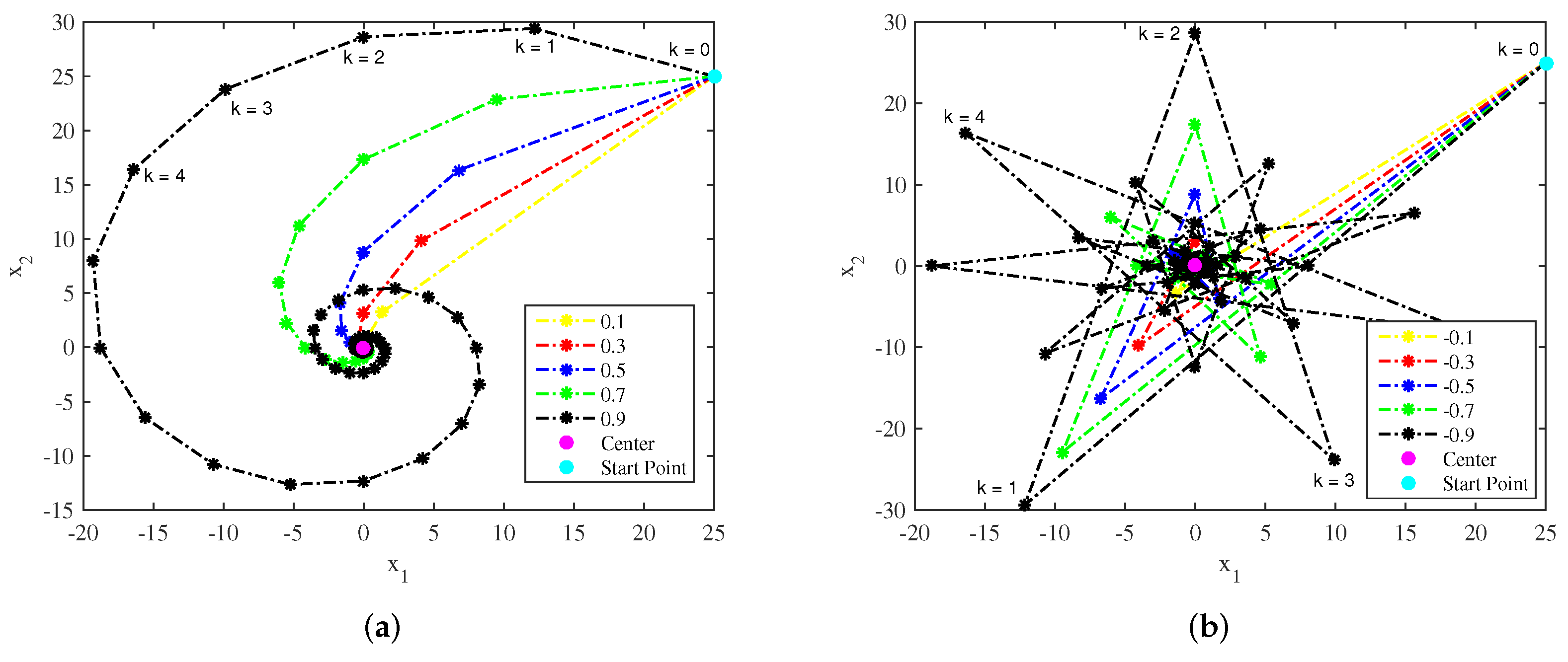
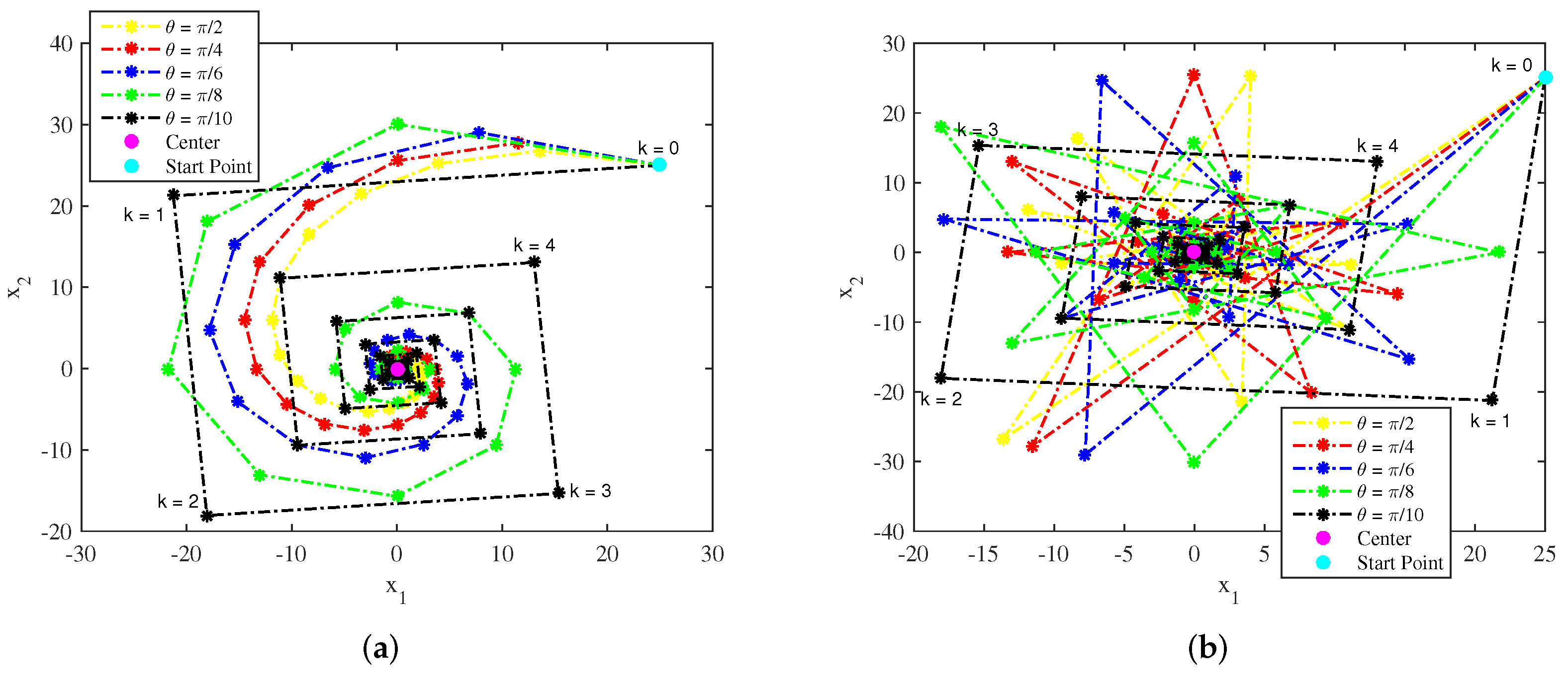
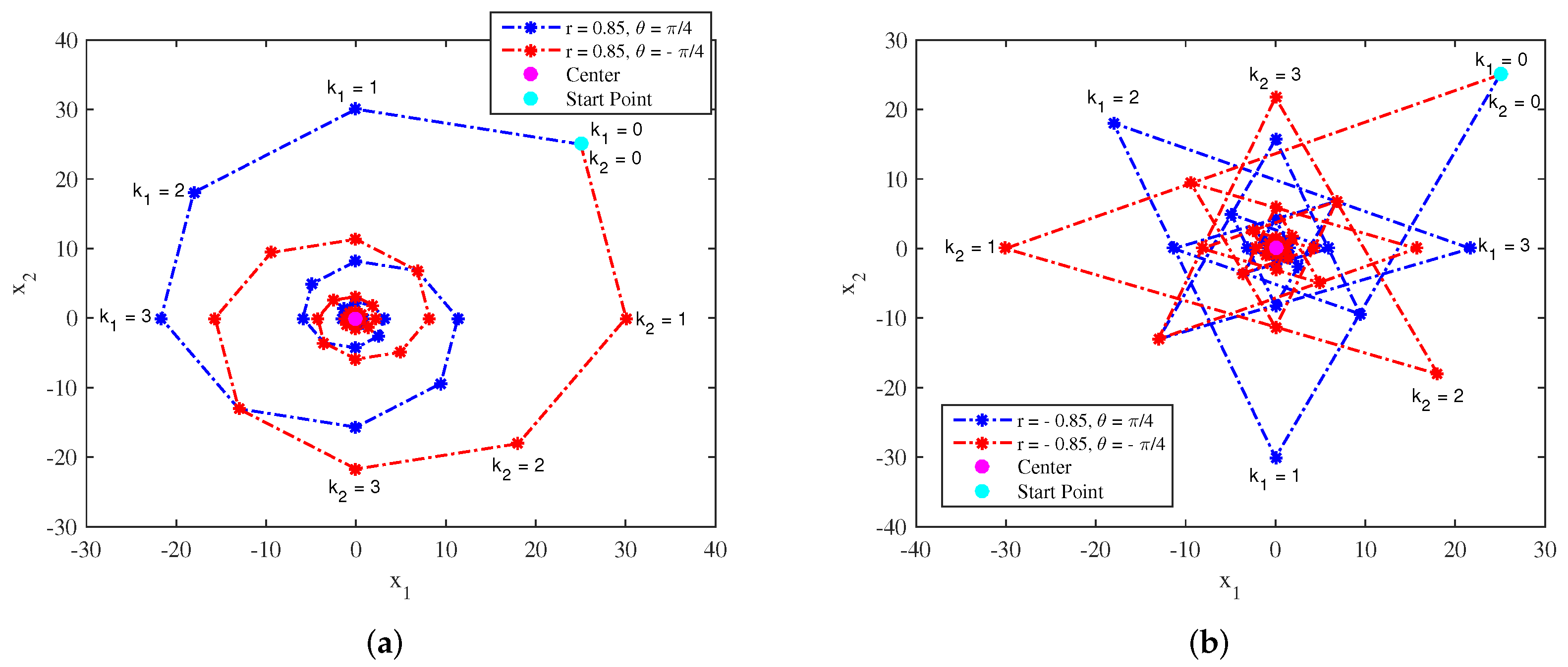
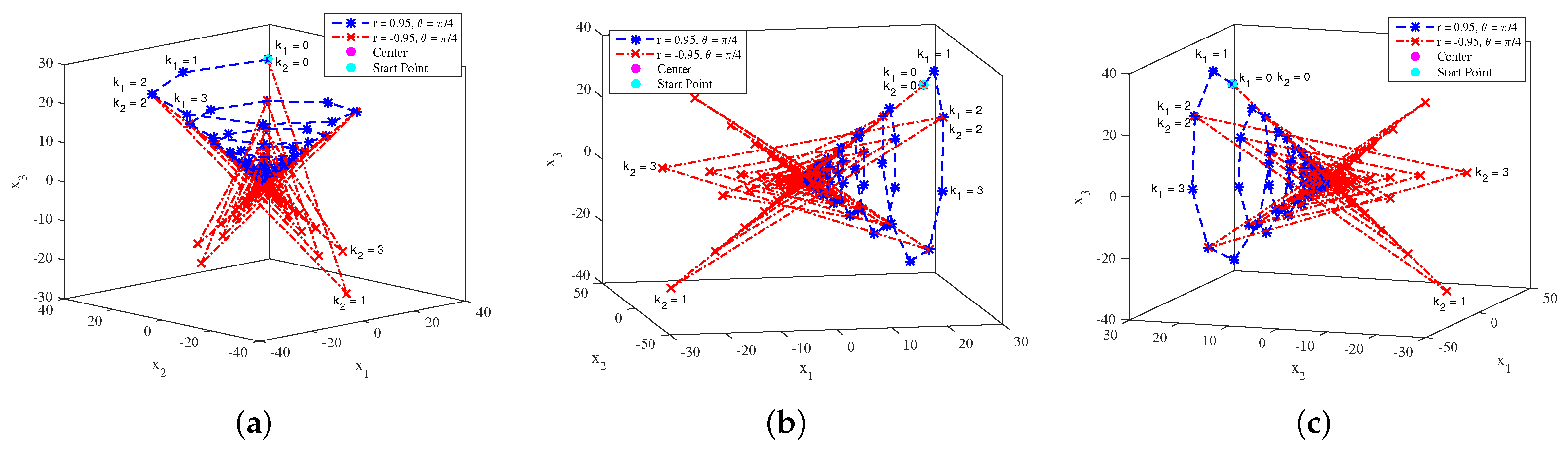
2.2. Concept

In the SDO algorithm, the multipoint search function for an n-dimensional system is formulated as [15],

$$x_{k+1}=r{R}^{\left(n\right)}\left(\theta \right)x_k-(r{R}^{\left(n\right)}\left(\theta \right)-I_n)x^{*},$$

(1)

where r is the spiral radius, $R^{\left(n\right)}\left(\theta \right)$ is the rotational matrix of order $n\times n$, $\theta$ is the spiral rotation angle, $I_n$ is the identity matrix of order $n\times n$, $x^{*}$ is the spiral center, $x_k$ and $x_{k+1}$ are the search point positions at iterations k and $k+1$, respectively.

The rotational matrix $R^{\left(n\right)}\left(\theta \right)$ for an n-dimensional case on an arbitrary $x_i{x}_j$-plane is given as [9,16,17],

$$R^{\left(n\right)}\left(\theta \right)=\left[\begin{array}{ccccccc}1& 0& 0& \cdots & 0& 0& 0\\ 0& 1& 0& \cdots & 0& 0& 0\\ 0& 0& cos\left({\theta }_{i,j}\right)& \cdots & -sin\left({\theta }_{i,j}\right)& 0& 0\\ ⋮& ⋮& ⋮& \ddots & ⋮& ⋮& ⋮\\ 0& 0& sin\left({\theta }_{i,j}\right)& \cdots & cos\left({\theta }_{i,j}\right)& 0& 0\\ 0& 0& 0& \cdots & 0& 1& 0\\ 0& 0& 0& \cdots & 0& 0& 1\end{array}\right],$$

(2)

where ${\theta }_{i,j}$ is the spiral rotation angle around the origin on $x_i{x}_j$-plane.

From (2), the only one possibility of rotational matrix $R^{\left(2\right)}\left(\theta \right)$ for a two-dimensional system on $x_1{x}_2$-plane is given as follows:

$$R^{\left(2\right)}\left(\theta \right)=\left[\begin{array}{cc}cos\left(\theta \right)& -sin\left(\theta \right)\\ sin\left(\theta \right)& cos\left(\theta \right)\end{array}\right].$$

(3)

On the other hand, the three possible combinations of rotational matrix $R^{\left(3\right)}\left(\theta \right)$ for a three-dimensional system on $x_1{x}_2$, $x_2{x}_3$, and $x_1{x}_3$-planes are respectively given as follows:

$$\begin{array}{ccc}\hfill R_{1,2}^{\left(3\right)}\left(\theta \right)& =& \left[\begin{array}{ccc}cos\left({\theta }_{1,2}\right)& -sin\left({\theta }_{1,2}\right)& 0\\ sin\left({\theta }_{1,2}\right)& cos\left({\theta }_{1,2}\right)& 0\\ 0& 0& 1\end{array}\right],\hfill \end{array}$$

(4)

$$\begin{array}{ccc}\hfill R_{2,3}^{\left(3\right)}\left(\theta \right)& =& \left[\begin{array}{ccc}1& 0& 0\\ 0& cos\left({\theta }_{2,3}\right)& -sin\left({\theta }_{2,3}\right)\\ 0& sin\left({\theta }_{2,3}\right)& cos\left({\theta }_{2,3}\right)\end{array}\right],\mathrm{and}\hfill \end{array}$$

(5)

$$\begin{array}{ccc}\hfill R_{1,3}^{\left(3\right)}\left(\theta \right)& =& \left[\begin{array}{ccc}cos\left({\theta }_{1,3}\right)& 0& -sin\left({\theta }_{1,3}\right)\\ 0& 1& 0\\ sin\left({\theta }_{1,3}\right)& 0& cos\left({\theta }_{1,3}\right)\end{array}\right].\hfill \end{array}$$

(6)

From (1), it is to be noted that the model generated the spiral trajectories around the center $x^{*}$ and these trajectories are classified into two types [18,19]:

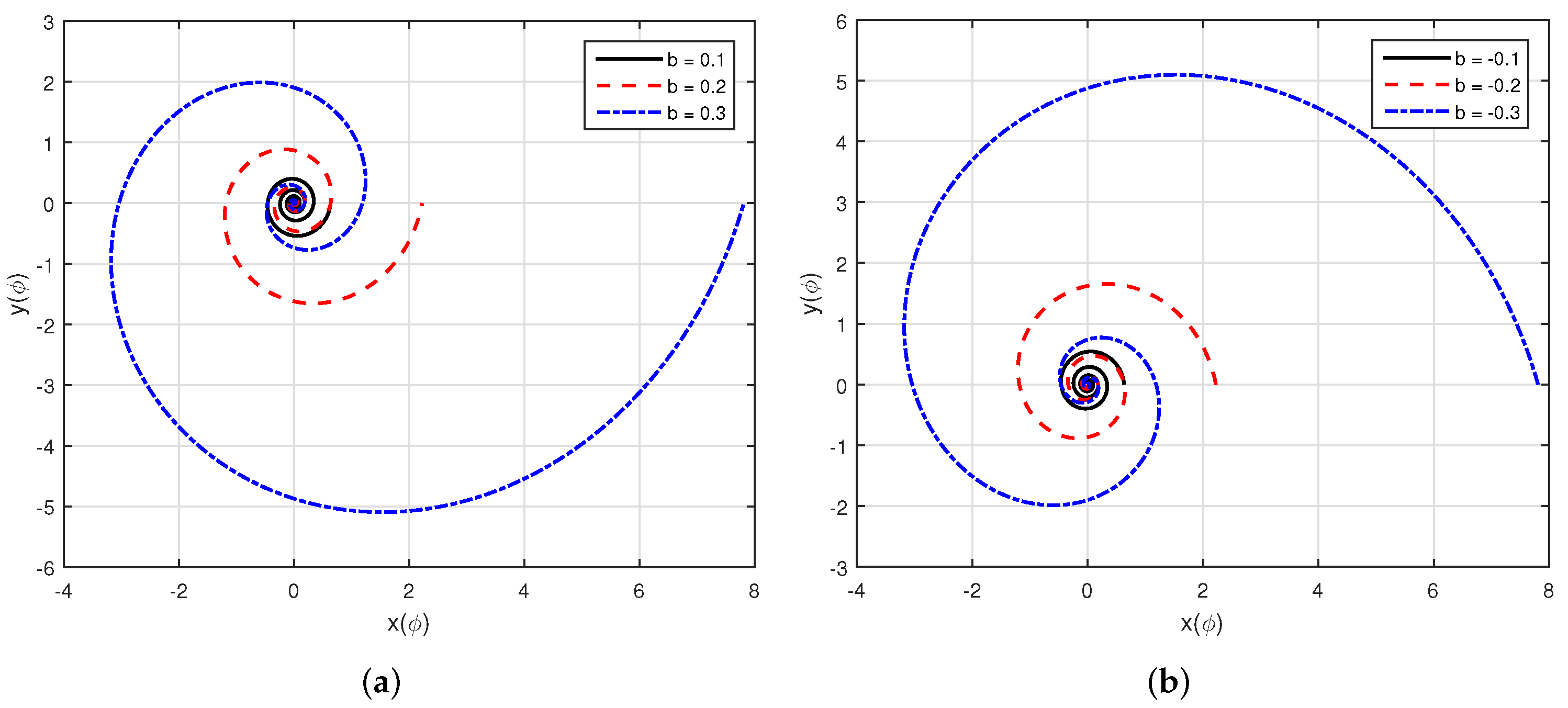
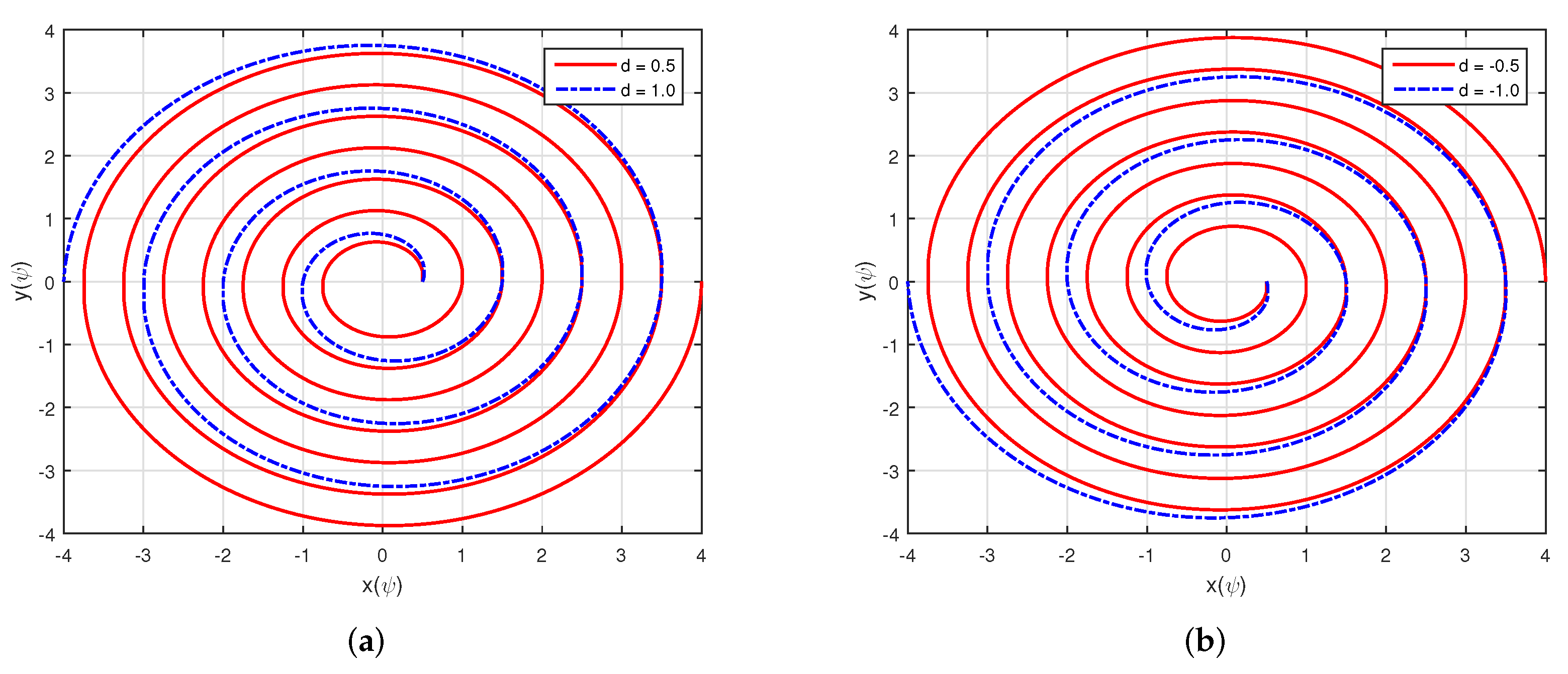
• If $r>1$ and $\theta \in (-\frac{\pi }{2},\frac{\pi }{2})$, the trajectory is a conventional spiral;
• If $r<1$ and $\theta \in (-\frac{\pi }{2},\frac{\pi }{2})$, the trajectory is a hypotrochoid spiral.

From the above classification, the spiral’s direction of rotation based on the value of $\theta$ is classified as follows:

• If $\theta \in (-\frac{\pi }{2},0)$, the rotation of trajectory is clockwise;
• If $\theta \in (0,\frac{\pi }{2})$, the rotation of trajectory is anticlockwise.

The spiral trajectories for a two-dimensional system for various values of $r\in [-1,1]$ and $\theta =\frac{\pi }{8}$ is shown in Figure 1. Similarly, the trajectories for various values of $\theta \in [-\frac{\pi }{2},\frac{\pi }{2}]$ and $r=0.85$ for conventional spiral and $r=-0.85$ for hypotrochoid spiral are shown in Figure 2. Further, the conventional and hypotrochoid spiral trajectories for both positive and negative values of $\theta$ are shown in Figure 3. In all these cases, the starting point used in the study is $(25,25)$.

Observing the notations $k=0$, $k=1$, ⋯, $k=4$ on spiral trajectories in Figure 1, Figure 2 and Figure 3, it can be noted that at each iteration, the spiral point from the starting point moves by an angle $\theta$ and then tends towards the center $x^{*}$. Thus, the net effect is the spiral movement of the initial point towards the center. The trajectories also depict the angle $\theta$, controlling the spiral curve. A smoother curve is achieved for smaller values of $\theta$, compared to the boxy curved with larger values of $\theta$ (refer to Figure 2a). The spiral trajectories in Figure 3 show the clockwise and anticlockwise spiral movement for negative and positive angles, respectively. On the other hand, the spiral radius r controls the spiral movement towards the center $x^{*}$. A quick movement of spiral towards the center is achieved for smaller values of r, compared to the slow movement with larger values of r (refer to Figure 1 and Figure 2). The hypotrochoid spirals shown in Figure 1b, Figure 2b, and Figure 3b are internal trajectories which are generated along a circle. The advantage of a hypotrochoid spiral over conventional spirals is it does not exceed the search space and can search most of the area in the search space.

In a similar way, the conventional and hypotrochoid spiral trajectories for a three-dimensional system with $r=0.95$ and $\theta =\frac{\pi }{4}$ are shown in Figure 4. The trajectory in Figure 4a on the $x_1{x}_2$-plane is obtained using the rotational matrix in (4). Similarly, the trajectories in Figure 4b,c on the $x_2{x}_3$ and $x_1{x}_3$-planes are obtained using the rotational matrices in (5) and (6), respectively. The starting point used is $(25,25,25)$ in all of these cases. The trajectories depict the conventional spiral with a positive r value and the hypotrochoid spiral with a negative r value. As the $\theta$ value is positive, all the spiral movements are anticlockwise. As mentioned earlier, the advantage of hypotrochoid spirals is they can search most of the area in the search space, as shown in Figure 4. The search space of a conventional spiral is only on the positive plane, while the hypotrochoid spirals search space is both negative and positive. Thus, the trajectories in the figure conclude that the hypotrochoid spirals can search most of the area in the search space.

3. Advances of Spiral Dynamics Optimization Algorithm

This section presents the recent adaptive, improved, and hybrid versions of the SDO algorithm.

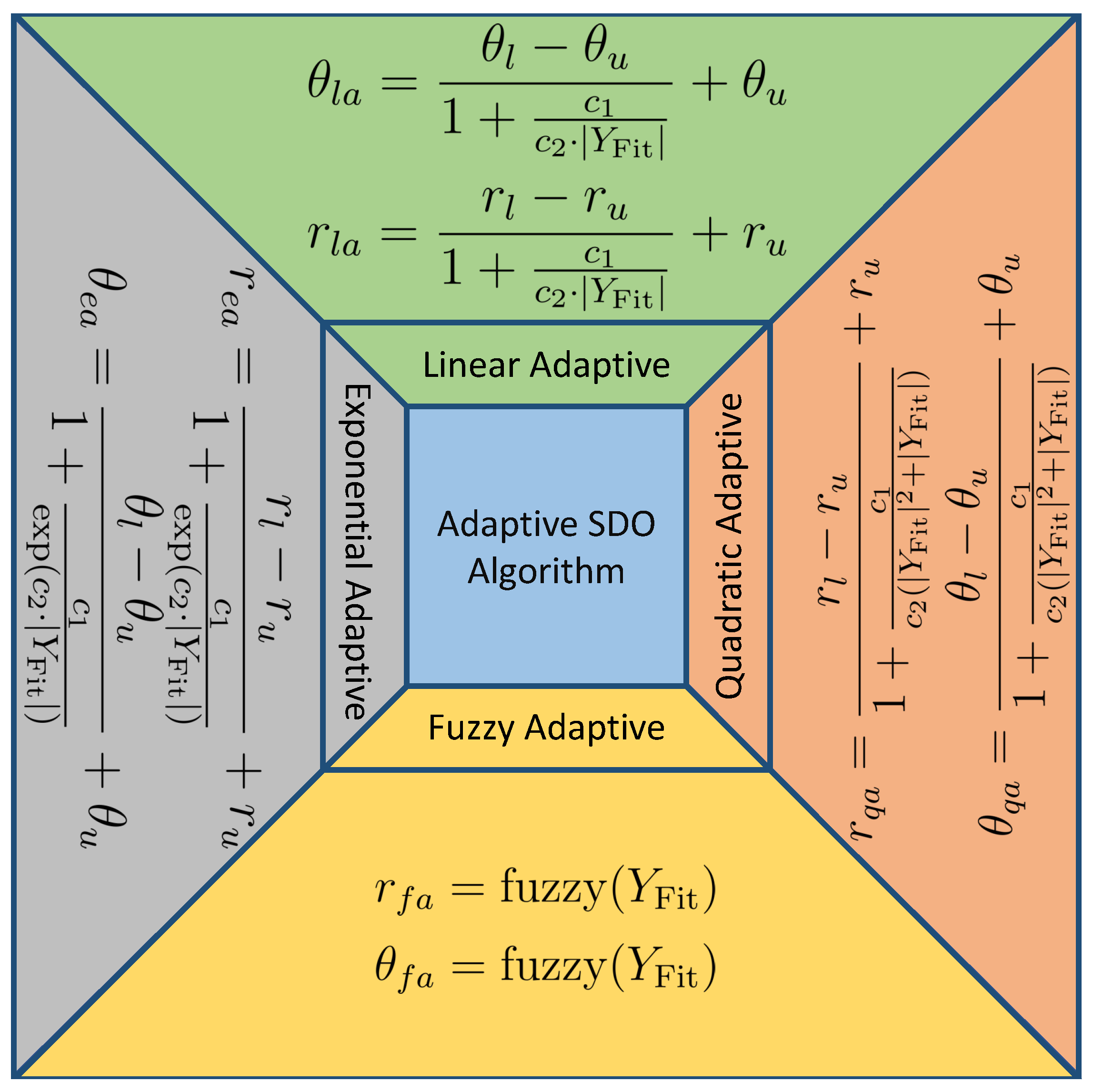
3.1. Adaptive Versions of Spiral Dynamics Optimization Algorithm

Researchers have developed the adaptive versions of the SDO algorithm by dynamically varying the spirals’ radius and angle based on the fitness value during each iteration. The four types of proposed adaptive approaches in the literature are linear, quadratic, exponential, and fuzzy [16,20,21]. The mathematical functions of spirals’ radius and angle using the proposed approaches are given in Figure 5.

In the figure, the notations are defined as follows:

• $r_{la}$ and ${\theta }_{la}$ are the computed radius and angle using linear adaptive approach;
• $r_{qa}$ and ${\theta }_{qa}$ are the obtained radius and angle using quadratic adaptive approach;
• $r_{ea}$ and ${\theta }_{ea}$ are the radius and angle obtained using exponential adaptive approach;
• $r_{fa}$ and ${\theta }_{fa}$ are the calculated radius and angle using fuzzy adaptive approach;
• $r_l\in [0,1]$ and $r_u\in [0,1]$ are the minimum and maximum radius of spiral;
• ${\theta }_l\in [0,1]$ and ${\theta }_u\in [0,1]$ are the minimum and maximum angles of spiral;
• $c_1$ and $c_2$ are constants;
• $\mathrm{fuzzy}(·)$ is the fuzzy logic mapping;
• $Y_{\mathrm{Fit}}$ is the difference between fitness value at a current iteration $f\left(x_i\left(k\right)\right)$ and best fitness $min\left(f\left(x_i\left(k\right)\right)\right)$, is defined as,

$$Y_{\mathrm{Fit}}=f\left(x_i\left(k\right)\right)-min\left(f\left(x_i\left(k\right)\right)\right).$$

(7)

In [17], using the linear adaptive approach in Figure 5, the authors have proposed the adaptive hypotrochoid SDO algorithm. The proposed algorithm performs best on various benchmark functions compared to conventional techniques. On the other hand, in [22], a self-adaptive approach is proposed for the SDO algorithm to update the spiral radius and angle during the optimization. The approach’s advantage is that all search points are updated by randomly tuning the parameter values in each iteration. Similarly, the authors of [23] have proposed an adaptive SDO by incorporating three mechanisms, such as (i) bi-considering updation, (ii) self-adaptive radius, and (iii) punish mechanisms. The proposed algorithm boosted the optimization efficiency and avoided trapping at the local optimal minima.

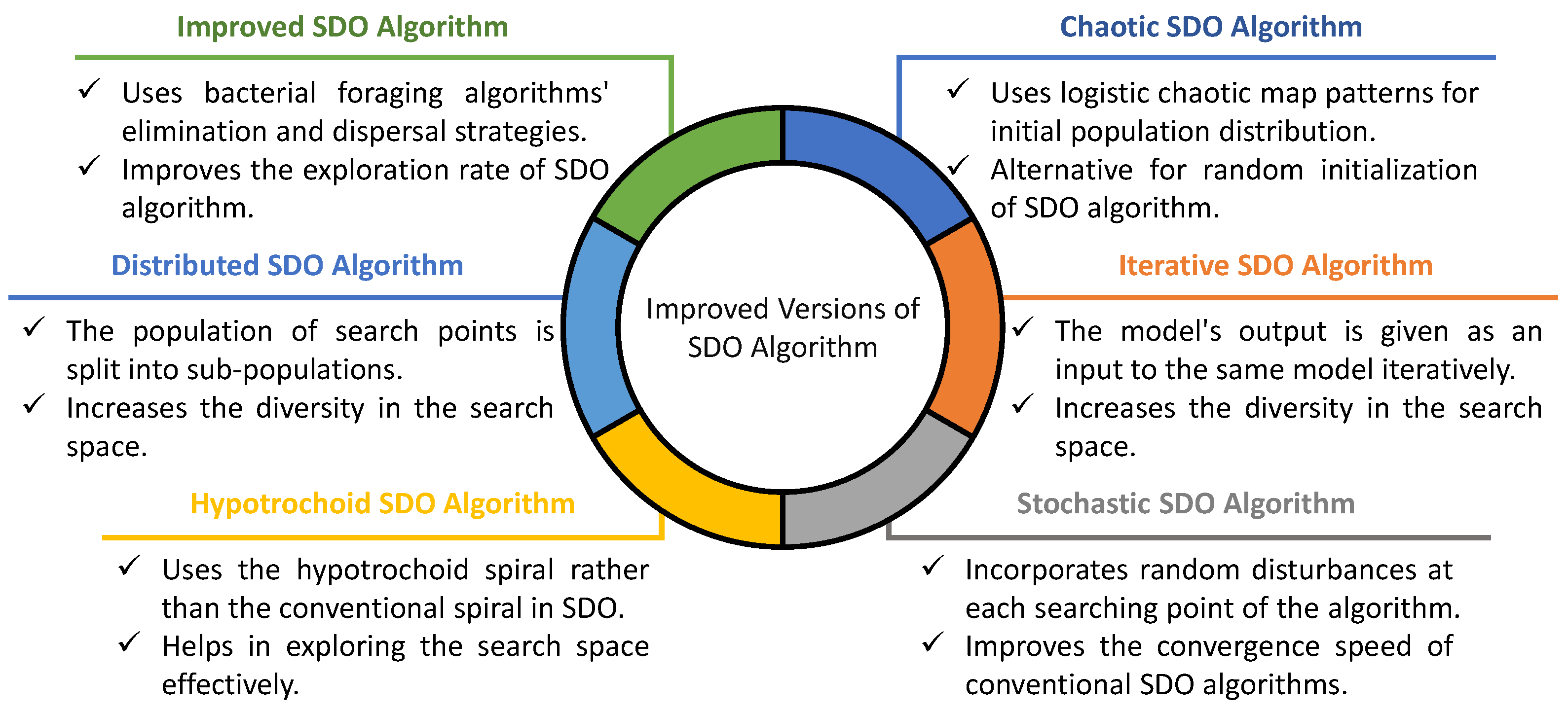
3.2. Improved Versions of Spiral Dynamics Optimization Algorithm

As mentioned earlier in Section 2.2, the algorithm settles into optimal local values at the end of the optimization process due to insufficient exploration of the conventional SDO’s search space. Thus, to avoid this problem, Nasir et al. have proposed the improved SDO algorithm using the bacterial foraging algorithms’ elimination–dispersal strategy [24,25]. In this enhanced version, the algorithm structure is kept the same. However, two new phases, namely elimination and dispersal, are introduced. Similarly, Hashim et al. have proposed the chaotic SDO algorithm logistic chaotic map patterns in the conventional SDO [26,27]. The chaotic map pattern helps in the initial population distribution rather than randomly in conventional SDO. Moreover, the search strategy of the artificial bee colony optimization algorithm is employed to improve the SDO’s exploration capability. The authors have also proposed the greedy SDO algorithm by incorporating the greedy selection stage and chaotic logistic map in the conventional SDO [28]. In this selection stage, the obtained solution is compared to the previous value for updating the spiral positions. The authors of [18,19] have proposed the hypotrochoid SDO algorithm in which the search points follow the hypotrochoid spiral rather than the conventional spiral in SDO. The proposed hypotrochoid SDO can explore the search space more effectively and explore the whole neighborhood of the optimal center. The experimental validation on optimal triaxial accelerometers placement in the Shanghai Tower in China [19], and sizing and layout of truss structures [18] has shown the better performance of hypotrochoid SDO than its predecessors.

The SDO algorithm in Section 2.2 is developed by utilizing a feature of the logarithmic spiral. This algorithm is also known as a deterministic or direct-solving metaheuristic optimization algorithm. One of the significant drawbacks of this algorithm is the slow convergence. Therefore, the authors of [29,30,31] have proposed a stochastic SDO algorithm by incorporating some random disturbances at each searching point of the algorithm. Similarly, the authors of [32] have introduced the iterative SDO algorithm for analyzing the information on blurred images. In this algorithm, the model’s output is given as an input to the same model iteratively. Thus, the optimization algorithm searches for the sharp image spirally with the blurred vision at the initial stage. On the other hand, the authors of [33] have proposed the distributed SDO algorithm to increase the diversity in the search space. In this conventional SDO algorithm, it is clear that the search points rotate spirally around the optimal center only. Thus, the algorithm falls into the local minimum quickly. However, in the proposed distributed SDO algorithm, the population of search points is split into sub-populations to increase diversity and capture the whole search space. The summary of all these approaches is given in Figure 6.

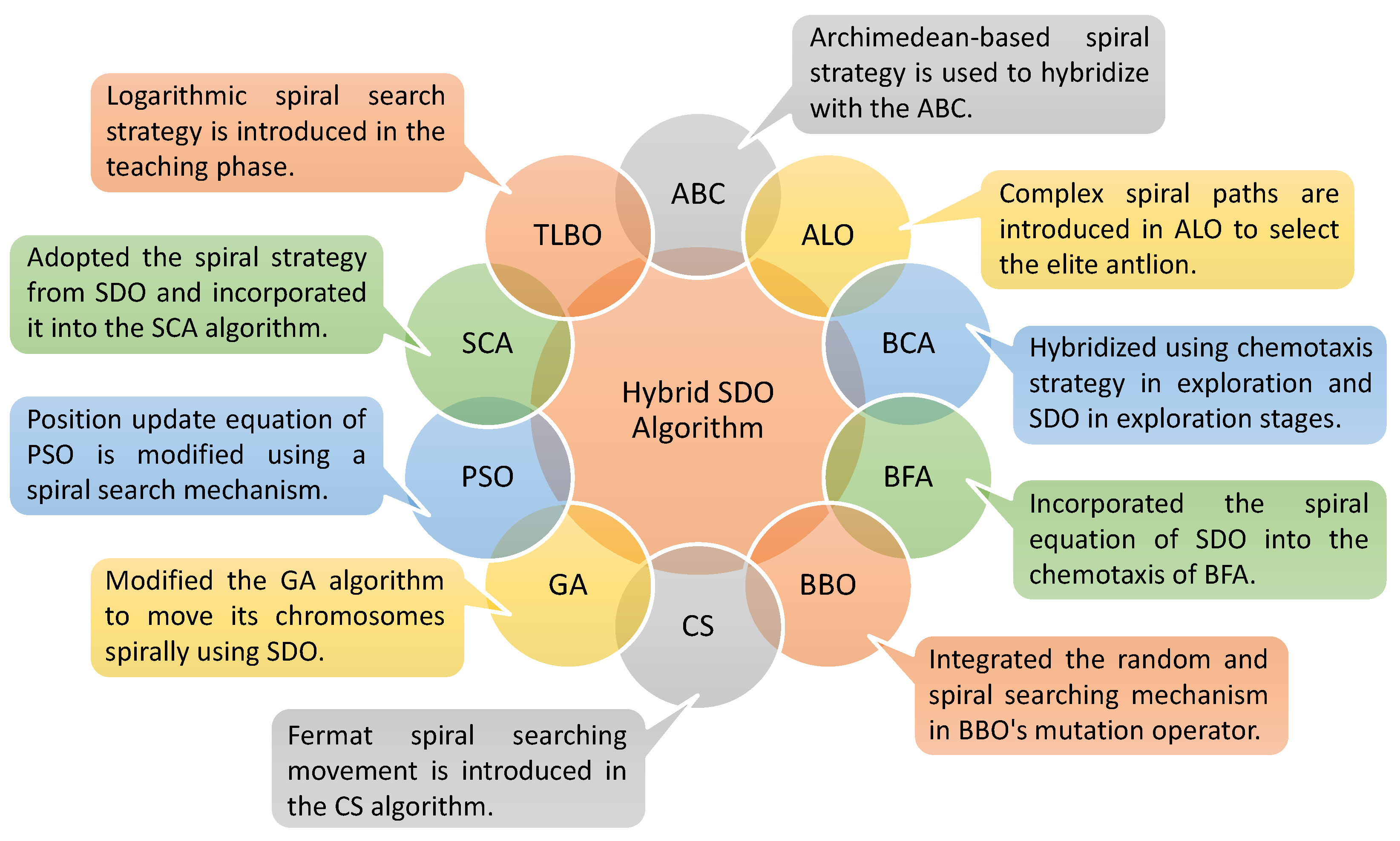
3.3. Hybrid Versions of Spiral Dynamics Optimization Algorithm

From the literature review, the following points are worth highlighting on the performance of the SDO algorithm. SDO has the advantages of a simple structure, few control parameters, and early diversification and intensification strategies. However, the SDO’s performance is poor in searching the whole search space [20,34], and the exploration mechanism of the SDO needs to be improved [35]. The algorithm gets trapped at optimal local minima easily [33].

Thus, to improve the performance of SDO, researchers have proposed the hybridization of SDO with other algorithms. Further, various algorithms’ performance has also been enhanced using SDO. The hybrid versions of the SDO algorithm presented in the literature used an artificial bee colony (ABC) [36,37], antlion optimization (ALO) [38], bacterial chemotaxis algorithm (BCA) [20,34,39], bacterial foraging algorithm (BFA) [35,40,41], biogeography-based optimization (BBO) [42], cuckoo search (CS) [43], genetic algorithm (GA) [44], particle swarm optimization (PSO) [45,46,47,48], sine-cosine algorithm (SCA) [49], and teaching–learning-based optimization (TLBO) [50], as shown in Figure 7. As shown in the figure, the excellent exploitation strategy of SDO is hybridized with the fast exploration strategy of another algorithm to balance both the exploitation and exploration phases.

Moreover, there are several other novel optimization algorithms in which spiral behavior or trajectory is used during the development of the algorithm. A detailed description of various spiral paths and a list of novel spiral path-inspired optimization algorithms are discussed in the following section.

4. Spiral Path Inspired Optimization Algorithms

The first part of this section presents the various spiral trajectories used to develop the optimization algorithms. Then, the list of different novel optimization algorithms created using these spirals is shown.

4.1. Spiral Paths

Patterns referred to as visible consistencies found in nature are trees, spirals, waves, etc. Visual patterns in nature are modeled using chaos theory, fractals, spirals, etc. In some natural patterns, the spirals and fractals are related. For instance, a variant of the logarithmic spiral, namely the Fibonacci spiral, is based on the golden ratio and Fibonacci numbers. As it is logarithmic, the curve at every scale appears the same and can be considered a fractal. Romanesco broccoli is an example of such Fractal spirals. The above patterns inspired researchers to develop optimization algorithms. Different types of spiral trajectories used in the research include:

• Archimedes spira;
• Cycloid spiral;
• Epitrochoid spiral;
• Hypotrochoid spiral;
• Logarithmic spiral;
• Rose spiral;
• Inverse spiral; and
• Overshoot spirals.

A detailed description of the five most widely used spirals, including Archimedes, logarithmic, rose, epitrochoid, and hypotrochoid, is provided underneath. This detailed description includes the coordinates on the $xy$-plane and trajectories showing the effect of each parameter on the $xy$-plane.

4.1.1. Logarithmic Spiral

The logarithmic spirals often appear in nature. For instance, the nautilus cutaway, Iceland’s low-pressure area, galaxies, and tropical cyclones arms usually take a logarithmic spiral shape. The logarithmic spiral is also known as equiangular or growth spiral because the spiral distance increases in geometric progression. The coordinates of a logarithmic spiral on $xy$-plane are given as follows [13,38]:

$$\begin{array}{c}\hfill x\left(\varphi \right)=a·e^{b\varphi }·cos\left(\varphi \right),y\left(\varphi \right)=a·e^{b\varphi }·sin\left(\varphi \right),\end{array}$$

(8)

where $\varphi$ is the angle, a and b are the arbitrary constants.

The logarithmic spiral for $a=0.18$, $\varphi$ from $-4\pi$ to $4\pi$, and various b values is shown in Figure 8. The spiral in Figure 8a is obtained for positive values of b, while Figure 8b is obtained for negative values. The trajectories in Figure 8 show that parameter b controls the tightness and the direction of the spiral. The trajectories in Figure 8a also depict the logarithmic spiral proprieties that for positive b values and $\varphi$ tends to $+\infty$, the spiral evolves in an anticlockwise direction. Whereas for the same b values and $\varphi$ tends to $-\infty$, the spiral evolves in a clockwise direction. However, for negative b values, the spiral evolves or twists in the opposite direction.

4.1.2. Archimedean Spiral

Archimedean spiral is another famous spiral that has been used in significant applications of engineering, biology, etc. The Archimedean spiral is also known as the arithmetic spiral. This spiral can be seen in nature in ferns, millipedes, and human fingerprints. The spiral trajectory is the locus of a point’s position that moves away from the fixed point with a constant speed along a line that rotates with a constant angular velocity. The coordinates of an Archimedean spiral on $xy$-plane is given as follows [13,38]:

$$\begin{array}{c}\hfill x\left(\psi \right)=(c+d·\psi )·cos\left(\psi \right),y\left(\psi \right)=(c+d·\psi )·sin\left(\psi \right),\end{array}$$

(9)

where c and d are constants that define the spirals initial radius and the successive turns difference, respectively.

The Archimedean spiral for $c=0.5$, $\psi$ from 0 to $-7\pi$, and various d values are shown in Figure 9. The trajectory in Figure 9a is obtained for positive values of d, while Figure 9b is obtained for negative values. As the initial radius is $c=0.5$, all the spirals are starting at this value, as shown in Figure 9. The spiral growth rate d controls the increment per revolution. Thus, the distance between successive turns is constant, which is equal to the value of d. Moreover, the parameter d controls the evolution of the spiral. The spiral in Figure 9a depicts that for positive d values, and the spiral evolves in an anticlockwise direction. Whereas for negative d values, the spiral evolves clockwise.

Observing the spirals in Figure 8 and Figure 9 shows a difference between the Archimedean and logarithmic spirals worth highlighting. In the Archimedean spiral, the intersection points of a ray from the origin on successive turnings have a constant separation distance. However, in a logarithmic spiral, these distance of intersection points on next turnings from the origin will form a geometric progression.

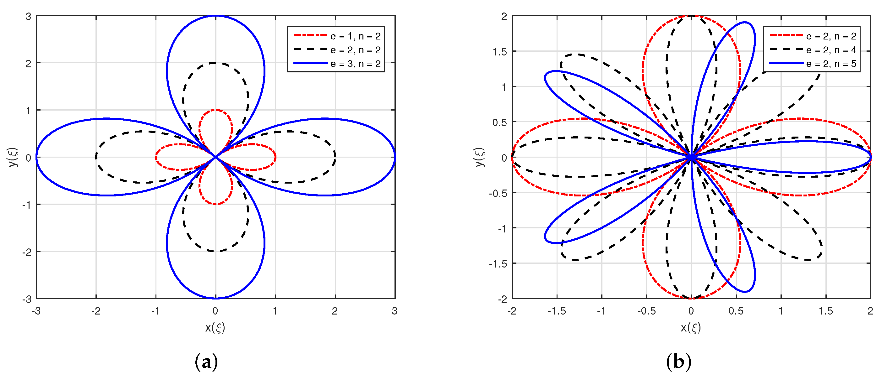
4.1.3. Rose Spiral

As the name suggests, the rose spiral is often seen in the unfurling of rose petals and holds the properties of symmetric and periodic arc curves. The coordinates of a rose spiral on $xy$-plane is given as follows [13,38]:

$$\begin{array}{c}\hfill x\left(\xi \right)=e·cos\left(n\xi \right)·cos\left(\xi \right),y\left(\xi \right)=e·cos\left(n\xi \right)·sin\left(\xi \right),\end{array}$$

(10)

where e and n are constants that define the pedal length and number, respectively.

The rose spiral with various values of e and n are shown in Figure 10. The spiral in Figure 10a is achieved for $n=2$ and multiple values of e. Similarly, the spiral in Figure 10b is obtained for $e=2$ and various values of n. In both cases, $\xi$ ranges from 0 to 2. The spirals in Figure 10a depict that parameter e controls the petal length. It is worth noting that as the value of e increases, the petal length increases. The spirals in Figure 10b also show that n controls petals’ number, size, and length. For an even value of n, the number of petals is $2n$. However, for odd values of n, the number of petals is only n.

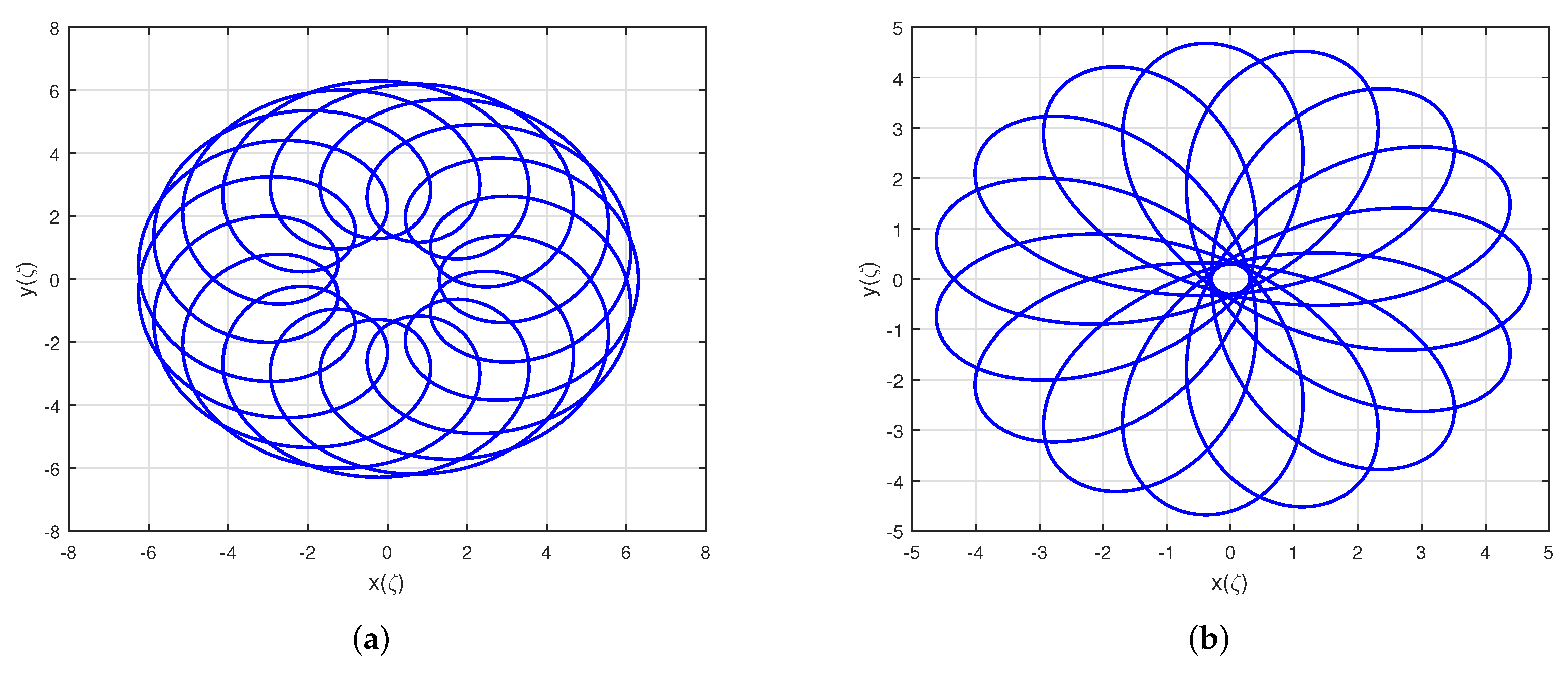
4.1.4. Epitrochoid and Hypotrochoid Spirals

Epitrochoid and hypotrochoid spirals are a family of curves generated by a point attached to a rolling circle. This rolling circle will roll out around the outside of a fixed circle to form an epitrochoid spiral. On the other hand, to create a hypotrochoid spiral, the rolling one will roll around inside the fixed one. Let ${\rho }_1$ and ${\rho }_2$ be the radii of rolling and fixed circles, respectively, and f is the distance between the point and rolling circle’s center. The coordinates of epitrochoid spiral on $xy$-plane is given as [13,38],

$$\begin{array}{cc}\hfill & x\left(\zeta \right)=({\rho }_2+{\rho }_1)·cos\left(\zeta \right)-f·cos\left(\frac{{\rho }_2+{\rho }_1}{{\rho }_1}\zeta \right),\mathrm{and}\hfill \\ \hfill & y\left(\zeta \right)=({\rho }_1+{\rho }_2)·sin\left(\zeta \right)-f·sin\left(\frac{{\rho }_1+{\rho }_2}{{\rho }_1}\zeta \right).\hfill \end{array}$$

(11)

Similarly, the coordinates of a hypotrochoid spiral on $xy$-plane is given as follows:

$$\begin{array}{cc}\hfill & x\left(\zeta \right)=({\rho }_2-{\rho }_1)·cos\left(\zeta \right)+f·cos\left(\frac{{\rho }_2-{\rho }_1}{{\rho }_1}\zeta \right),\mathrm{and}\hfill \\ \hfill & y\left(\zeta \right)=({\rho }_2-{\rho }_1)·sin\left(\zeta \right)-f·sin\left(\frac{{\rho }_2-{\rho }_1}{{\rho }_1}\zeta \right).\hfill \end{array}$$

(12)

The trajectories of epitrochoid and hypotrochoid spirals for ${\rho }_1=0.8$, ${\rho }_2=3$, $d=2.5$, and $\zeta$ ranging from 0 to $10\pi$ is shown in Figure 11a,b, respectively. In both spirals, it should be noted that $\zeta$ significantly affects the spiral’s shape. If the considered $\zeta$ ranges from 0 to $2\pi$, the rolling circle will revolve only once around the fixed circle. Thus, it is not possible to obtain the whole pattern of the spiral. These spirals can be drawn using Spirograph toys and often appear in nature. For instance, the planets orbit in a geocentric system, and Wankel engines’ combustion chambers take these spiral shapes.

4.2. Spiral Path-Based Optimization Algorithms

Over the years, researchers have developed various novel optimization algorithms in which the spiral motion has been used while mimicking the system’s behavior. Further, an improved version of multiple algorithms is also proposed using spiral trajectories to improve the performance of conventional techniques.

Table 1. List of spiral path-inspired optimization algorithms.

Ref.	Year	Algorithm	Author	Inspiration	Spiral Type	Source Code Link
[40,41]	2010	Spiral Bacterial Foraging Optimization Algorithm	Alireza Kasaiezadeh et al.	E. coli bacteria foraging behavior	Spiral	–
[8]	2011	Galaxy-Based Search Algorithm	Hamed Shah-Hosseini	Arms of the spiral galaxy	Spiral	–
[51]	2014	Hurricane-Based Optimization Algorithm	Isamil Rbouh et al.	Behavior of hurricanes, radial wind, and pressure profiles	Logarithmic spiral	–
[52]	2015	Moth–flame Optimization Algorithm	Seyedali Mirjalili	Moths’ navigation behavior around the flame	Logarithmic spiral	https://seyedalimirjalili.com/mfo (accessed on 1 December 2021)
[53]	2016	Whale Optimization Algorithm	Seyedali Mirjalili	Whales’ hunting bubble net phenomenon	Logarithmic spiral	https://seyedalimirjalili.com/woa (accessed on 1 December 2021)
[54]	2017	Moth Swarm Optimization Algorithm	Al-Attar Ali Mohamed et al.	Moths orientation towards the moonlight	Logarithmic spiral	https://mathworks.com/matlabcentral/fileexchange/57822 (accessed on 1 December 2021)
[50]	2018	Improved Teaching–Learning-Based Optimization Algorithm	Zhuoran Zhang et al.	effect of teacher influence on learners	Logarithmic spiral	–
[55]	2018	Developed Grey Wolf Optimization Algorithm	Mostafa Abdo et al.	Grey wolves leadership and hunting strategies	Logarithmic spiral	–
[56]	2019	Seagull Optimization Algorithm	Gaurav Dhiman et al.	Seagulls’ migration and attacking behavior	3D logarithmic spiral	https://mathworks.com/matlabcentral/fileexchange/75180 (accessed on 1 December 2021)
[57]	2019	Emperor Penguins Colony Optimization Algorithm	Sasan Harifi et al.	Emperor penguins behavior	Logarithmic spiral	–
[36,37]	2019	Spiral Artificial Bee Colony Algorithm	Sonal Sharma et al.	Honey bee swarms’ intelligent foraging behavior	Logarithmic and Archimedean spirals	–
[58]	2019	Sooty Tern Optimization Algorithm	Gaurav Dhiman et al.	Sooty terns’ migration and attacking behaviors	Spiral	https://mathworks.com/matlabcentral/fileexchange/76667 (accessed on 1 December 2021)
[59]	2019	Whirlpool Algorithm	Yuanyang Zou et al.	Physical phenomenon of whirlpool	Spiral	–
[60]	2020	Improved Crow Search Algorithm	Xiaoxia Han et al.	Crows intelligent behavior of searching, hiding and retrieving food	Logarithmic Spiral	–
[38]	2020	Improved Ant Lion Optimization Algorithm	M. W. Guo et al.	Natural hunting phenomenon of antlions	Archimedes, Cycloid, Epitrochoid, Hypotrochoid, Logarithmic, Rose, Inverse, and Overshoot spirals	–
[61]	2020	Manta Ray Foraging Optimization Algorithm	Weiguo Zhao et al.	Manta rays intelligent behavior	Logarithmic spiral	https://www.mathworks.com/matlabcentral/fileexchange/73130 (accessed on 1 December 2021)
[62]	2020	Bald Eagle Search Optimization Algorithm	H. A. Alsattar et al.	Bald eagles hunting behavior	Spiral	https://mathworks.com/matlabcentral/fileexchange/86862 (accessed on 1 December 2021)
[63]	2020	Improved Firefly Algorithm	Jinran Wu et al.	Fireflies’ flashing behavior	Logarithmic spiral	https://github.com/wujrtudou/AdaptiveFireflyAlgorithm (accessed on 1 December 2021)
[64]	2021	Spiral Water Cycle Algorithm	Heba F. Eid et al.	Natural hydrological cycle process	Hyperbolic spiral	–
[65]	2021	Improved Slap Swarm Optimization Algorithm	Diab Mokeddem	Behavior of slap chains	Logarithmic spiral	–
[66]	2021	Spiral Flying Sparrow Search Algorithm	Chengtian Ouyang et al.	Sparrow’s behaviors during group wisdom, antipredation, and foraging	Logarithmic spiral	–
[67]	2021	Spiral Grasshopper Optimization Algorithm	Zhangze Xu et al.	Grasshoppers foraging and swarming behavior	Logarithmic spiral	–
[68]	2021	Aquila Optimization Algorithm	Laith Abualigah et al.	Aquilas’ behavior during prey catching	Spiral	https://www.mathworks.com/matlabcentral/fileexchange/89381 (accessed on 1 December 2021)
[69]	2021	Spiral Spotted Hyena Optimization Algorithm	Vijay Kumar et al.	Spotted hyenas behavior during hunting	Logarithmic spiral	–
[70]	2021	Spiral Chicken Swarm Optimization Algorithm	Miao Li et al.	Chicken swarms’ hierarchical order and its behaviors	Logarithmic spiral	–
[71]	2021	Golden Eagle Optimization Algorithm	Abdolkarim Mohammadi-Balani et al.	Golden eagles’ intelligent behavior during hunting	Spiral	https://mathworks.com/matlabcentral/fileexchange/84430 (accessed on 1 December 2021)

provides the list of spiral path-inspired optimization techniques, including the inspiration of developing the algorithm, the type of spiral used, and the source code links.

For example, a detailed description of four novel optimization algorithms in which spiral trajectory has been used in the development is explained underneath. The chosen novel optimizations algorithms list includes moth–flame, whale, seagull, and Aquila. Further, a detailed description of four improved optimization algorithms using spiral trajectories is also explained in this section. The enhanced optimization algorithms are the water cycle, antlion, slap swarm, and sparrow search. Some of these algorithms have been widely used by various researchers recently, and others have been developed newly, thus selected for the detailed explanation.

4.2.1. Moth–Flame Optimization Algorithm

The moth–flame optimization algorithm was developed in 2015 by Seyedali Mirjalili from the behavior of moths’ navigation around the light/flame in a spiral path [52,72,73]. The application of a logarithmic spiral to mimic the moths’ transverse orientation property around the flame in this algorithm is explained underneath. In the algorithm, the initial moths’ positions will be updated with respect to flames using the logarithmic spiral as follows [52,74]:

$$m_{i,j}=\left\{\begin{array}{cc}{D}_{i,j}·e^{b\tau }·cos\left(2\pi \tau \right)+f_{i,j},\hfill & \mathrm{for}i\le F_N\hfill \\ D_{i,j}·e^{b\tau }·cos\left(2\pi \tau \right)+f_{N,j},\hfill & \mathrm{for}i>F_N\hfill \end{array}\right.,$$

(13)

where $m_{i,j}$, $f_{i,j}$, and $D_{i,j}$ are the positions of jth variable of ith moth, flame, and distance between the moth and its corresponding flame, N is the total number of flames. Further, b and $\tau$ are the parameters of logarithmic spiral (refer to Section 4.1.1).

The major drawback of this algorithm is the premature convergence at optimal local solutions during the search process. Moreover, they cannot be applied to permutation problems as it is developed for continuous search space [75]. As mentioned in Table 1, the source code of this optimization algorithm created using MATLAB for both single and multiobjective problems is made publicly available by the developer on his website at https://seyedalimirjalili.com/mfo (accessed on 1 December 2021). Further, the links for the source code using other platforms, such as Python, C++, and R studio, are also available on the same website.

4.2.2. Whale Optimization Algorithm

The whale optimization algorithm is a novel metaheuristic algorithm developed in 2016 by Seyedali Mirjalili and Andrew Lewis to mimic whales’ hunting bubble net phenomenon in a spiral motion [53,76,77,78,79]. The algorithm is a model of capturing whales’ behavior during the encircling, attacking, and searching of prey. During the encircling phase, all the whales’ positions will be updated to move towards the best whale position, which is near to the target and is given as,

$$\overrightarrow{X}(i+1)={\overrightarrow{X}}^{*}\left(i\right)-\overrightarrow{\mathrm{A}}·|\overrightarrow{\mathrm{C}}·{\overrightarrow{X}}^{*}\left(i\right)-\overrightarrow{X}\left(i\right)|.$$

(14)

During the phase of attacking the prey, the whales move spirally using the bubble net movement phenomenon. Thus, position updation of whales during this phenomenon in logarithmic spiral motion is as follows:

$$\overrightarrow{X}(i+1)=|{\overrightarrow{X}}^{*}\left(i\right)-\overrightarrow{X}\left(i\right)|·e^{bl}·cos\left(2\pi l\right){\overrightarrow{X}}^{*}\left(i\right).$$

(15)

Finally, the whales will choose either encircling or attacking during the searching of prey, which can be achieved using the following model:

$$\overrightarrow{X}(i+1)=\left\{\begin{array}{cc}{\overrightarrow{X}}^{*}\left(i\right)-\overrightarrow{\mathrm{A}}·|\overrightarrow{\mathrm{C}}·{\overrightarrow{X}}^{*}\left(i\right)-\overrightarrow{X}\left(i\right)|,\hfill & p<0.5,\hfill \\ |{\overrightarrow{X}}^{*}\left(i\right)-\overrightarrow{X}\left(i\right)|·e^{bl}·cos\left(2\pi l\right){\overrightarrow{X}}^{*}\left(i\right),\hfill & p\ge 0.5.\hfill \end{array}\right.$$

(16)

Therefore, the position updation of all the whales during all three phases is summarized as,

$$\overrightarrow{X}(i+1)=\left\{\begin{array}{cc}\left\{\begin{array}{cc}{\overrightarrow{X}}^{*}\left(i\right)-\overrightarrow{\mathrm{A}}·|\overrightarrow{\mathrm{C}}·{\overrightarrow{X}}^{*}\left(i\right)-\overrightarrow{X}\left(i\right)|,\hfill & \overrightarrow{\mathrm{A}}<1,\hfill \\ {\overrightarrow{X}}_{\mathrm{r}}\left(i\right)-\overrightarrow{\mathrm{A}}·|\overrightarrow{\mathrm{C}}·{\overrightarrow{X}}_{\mathrm{r}}\left(i\right)-\overrightarrow{X}\left(i\right)|,\hfill & \overrightarrow{\mathrm{A}}\ge 1,\hfill \end{array}\right.\hfill & p<0.5,\hfill \\ |{\overrightarrow{X}}^{*}\left(i\right)-\overrightarrow{X}\left(i\right)|·e^{bl}·cos\left(2\pi l\right){\overrightarrow{X}}^{*}\left(i\right),\hfill & p\ge 0.5,\hfill \end{array}\right.,$$

(17)

where the vectors ${\overrightarrow{X}}^{*}\left(i\right)$ is the closest whale’s position to the prey, $\overrightarrow{X}\left(i\right)$ and $\overrightarrow{X}(i+1)$ are the whales’ positions at ith and $i+1^{\mathrm{th}}$ iterations, $\overrightarrow{\mathrm{A}}$ and $\overrightarrow{\mathrm{C}}$ are the coefficients, b and l are the parameters of logarithmic spiral (refer to Section 4.1.1). Further, it is to be noted that for $\overrightarrow{\mathrm{A}}\ge 1$, positions updation has been achieved using ${\overrightarrow{X}}_{\mathrm{r}}\left(i\right)$, a random position vector at ith iteration.

This whale optimization algorithm has the drawbacks of lower accuracy, slow convergence, and being trapped into optimal local solutions and cannot solve higher-dimensional problems effectively [80]. As given in Table 1, the source codes of this optimization algorithm for single-objective problems using MATLAB, Python, C++, and R are publicly available at https://seyedalimirjalili.com/woa (accessed on 1 December 2021).

4.2.3. Seagull Optimization Algorithm

Gaurav Dhiman et al. proposed the seagull optimization algorithm in 2019 to mimic the seagulls’ migration and hunting behavior [56]. The algorithm is a mathematical model of seagulls’ behavior in two stages, namely migration and attack. During the stage of natural attacking, the seagulls maintain spiral behavior in the air. The coordinates of this spiral behavior in x, y, and z planes are modeled as follows:

$$\begin{array}{c}\hfill x=u·e^{kv}·cos\left(k\right),y=u·e^{kv}·sin\left(k\right),z=u·e^{kv}·k,\end{array}$$

(18)

where $k\in [0,2\pi ]$ is the spiral angle, u and v are the arbitrary constants.

The seagull optimization algorithm has the significant drawback of weak population diversity during the search process [81]. The link to the MATLAB-based source code of this optimization algorithm is given in Table 1.

4.2.4. Aquila Optimization Algorithm

The Aquila optimization algorithm was proposed in 2021 by Laith Abualigah et al. to mimic Aquila’s behavior during prey catching [68]. The algorithm constitutes four stages: (i) expanded exploration, (ii) narrowed exploration, (iii) expanded exploitation, and (iv) narrowed exploitation. During the stage of narrowed exploration, the Aquila rotates over a target prey for a short glide attack. This behavior is modeled as follows:

$$X(t+1)=X_{best}\left(t\right)·Levy\left(\right)+X_r\left(t\right)+(y-x)·rand\left(\right),$$

(19)

where $X_r\left(t\right)$ and $X_{best}\left(t\right)$ are the random and best solutions at tth iteration, $X(t+1)$ solution at ${(t+1)}^{\mathrm{th}}$ iteration, $rand\left(\right)\in (0,1]$ is the random number, and $Levy\left(\right)$ is the Lévy distribution. Further, x and y are the Cartesian coordinates of the spiral with radius r and angle l given as follows:

$$\begin{array}{c}\hfill x=rsin\left(l\right),y=rcos\left(l\right).\end{array}$$

(20)

From the above, it is to be highlighted that the Levy flight’s effect is relatively weak. Thus, the algorithm has insufficient local exploitation ability [82]. The MATLAB and Java-based source code link of this optimization algorithm for single-objective problems is given in Table 1.

4.2.5. Water Cycle Optimization Algorithm

The water cycle optimization algorithm was proposed in 2012 by Eskandar et al. to mimic the natural hydrological cycle process [10,83,84]. The algorithm simulates the stream and river flow, rainfall, and evaporation into the sea. In this algorithm, the position update of (a) streams flow to the rivers, (b) streams flow to the sea, and (c) rivers flow to the sea are respectively given as follows:

$$X_{st}(i+1)=X_{st}\left(i\right)+rand\left(\right)·C·(X_r\left(i\right)-X_{st}\left(i\right)),$$

(21)

$$X_{st}(i+1)=X_{st}\left(i\right)+rand\left(\right)·C·(X_{se}\left(i\right)-X_{st}\left(i\right)),$$

(22)

$$X_r(i+1)=X_r\left(i\right)+rand\left(\right)·C·(X_{se}\left(i\right)-X_r\left(i\right)),$$

(23)

where $X_{st}\left(i\right)$, $X_r\left(i\right)$ and $X_{se}\left(i\right)$ are the positions of stream, river, and sea at ith iteration, $X_{st}(i+1)$, $X_r(i+1)$, and $X_{se}(i+1)$ are the positions of stream, river, and sea at ${(i+1)}^{\mathrm{th}}$ iteration, $C\in [1,2]$ is the constant value and $rand\left(\right)\in (0,1]$ is the random number.

The MATLAB-based source code of this conventional optimization algorithm for both constrained and unconstrained problems, including several improved versions and multiobjective problems, are made publicly available by the researcher on his website at https://ali-sadollah.com/water-cycle-algorithm-wca/ (accessed on 1 December 2021).

The algorithm has insufficient exploitation ability, and thus, in [64], the authors have integrated the hyperbolic spiral, which helps improve the exploitation ability of the algorithm. Therefore, modified position update equations using the hyperbolic spiral are given as follows:

$$X_{st}(i+1)=X_{st}\left(i\right)+|X_r\left(i\right)-X_{st}\left(i\right)|·cos\left(2\pi l\right)/l,$$

(24)

$$X_{st}(i+1)=X_{st}\left(i\right)+|X_{se}\left(i\right)-X_{st}\left(i\right)|·cos\left(2\pi l\right)/l,$$

(25)

$$X_r(i+1)=X_r\left(i\right)+|X_{se}\left(i\right)-X_r\left(i\right)|·cos\left(2\pi l\right)/l,$$

(26)

where $l\in [-1,1]$ is the parameter of hyperbolic spiral, which is an uniformly distributed random number.

4.2.6. Ant Lion Optimization Algorithm

Seyedali Mirjalili proposed the antlion optimization algorithm in 2015 to mimic the natural hunting phenomenon of antlions [85,86,87,88]. The algorithm is a model of capturing the following ants and antlions behaviors: (i) the ants’ random walk behavior and gets trapped in antlions pits and (ii) the antlions’ hunting behaviors include building traps, sliding ants towards them, catching, rebuilding pits, and elitism. The algorithm retains the best antlion with optimal fitness value, elitism, and the corresponding antlion is called elite antlion. Thus, the elite and selected antlions update their position randomly as follows:

$${\mathrm{Ant}}_i\left(t\right)=\frac{R_e\left(t\right)+R_a\left(t\right)}{2},$$

(27)

where $R_e\left(t\right)$ and $R_a\left(t\right)$ are the elite and selected antlions random walk during tth iteration.

The MATLAB, Python, and R software-based source codes of this conventional optimization algorithm for both single and multiobjective problems are made publicly available by Seyedali Mirjalili on his website at https://seyedalimirjalili.com/alo (accessed on 1 December 2021).

In [38], the authors proposed an improved version of this algorithm. In this enhanced version, the elite and selected antlions update their position using eight spiral complex paths instead of moving in randomly to improve the convergence speed and performance. These spiral trajectories include Archimedes, cycloid, epitrochoid, hypotrochoid, logarithmic, rose, inverse, and overshoot spirals. For an example case, the values of $R_e\left(t\right)$ and $R_a\left(t\right)$ are computed using logarithmic spiral as,

$$\begin{array}{c}\hfill R_e\left(t\right)=D_1·e^{b_{1}t}cos\left(2\pi t_1\right),R_a\left(t\right)=D_1·e^{b_{1}t}sin\left(2\pi t_1\right),\end{array}$$

(28)

where $D_1$, $b_1$, and $t_1$ are the parameters of logarithmic spiral (see Section 4.1.1).

Similarly, using the Archimedes spiral, the values of $R_e\left(t\right)$ and $R_a\left(t\right)$ are computed as follows:

$$\begin{array}{c}\hfill R_e\left(t\right)=D_2+b_2·t_2·cos\left(2\pi t_2\right),R_a\left(t\right)=D_2+b_2·t_2·sin\left(2\pi t_2\right),\end{array}$$

(29)

where $D_2$, $b_2$, and $t_2$ are the parameters of Archimedes spiral (see Section 4.1.2).

4.2.7. Slap Swarm Optimization Algorithm

Slap swarm optimization algorithm was developed in 2017 by Seyedali Mirjalili et al. to mimic the behavior of slap chains, which is searching for target food [89,90,91,92]. In the slap chain, the first slap is the leader, and all the other slaps follow the leader. In the algorithm, the update equations for the leader and followers’ positions during the searching of target food are as follows:

$$X_i^1=\left\{\begin{array}{cc}{\mathrm{F}}_i+r_1(({\mathrm{UB}}_i-{\mathrm{LB}}_i)r_2+{\mathrm{LB}}_i),\hfill & \mathrm{if}{r}_3\ge 0,\hfill \\ {\mathrm{F}}_i-r_1(({\mathrm{UB}}_i-{\mathrm{LB}}_i)r_2+{\mathrm{LB}}_i),\hfill & \mathrm{if}{r}_3<0,\hfill \end{array}\right.,$$

(30)

$$X_i^j=0.5(X_i^j+X_i^{j-1}),j\ge 2,$$

(31)

where $X_i^1$ and $X_i^j$ are the positions of leader and followers, $F_i$ is the target food, ${\mathrm{LB}}_i$ and ${\mathrm{UB}}_i$ are the lower and upper bounds of ith dimension, $r_1$, $r_2$, and $r_3$ are random numbers.

The MATLAB-based source code of this optimization algorithm for both single and multiobjective problems is made publicly available by the developer on his website at https://seyedalimirjalili.com/ssa (accessed on 1 December 2021). Further, the links for the source code using Python and R are also available on the same website.

However, in [65], it is stated that the conventional slap swarm optimization algorithm (SSOA) has a slower convergence and gets trapped at local optima. Thus, the authors have proposed an improved SSOA using a logarithmic spiral. In this improved algorithm, the followers’ positions are updated using a logarithmic spiral as follows:

$$X_i^j=0.5(X_i^j+X_i^{j-1})·e^{b\theta }·cos\left(2\pi \theta \right),j\ge 2,$$

(32)

where b and $\theta$ are the parameters of logarithmic spiral (refer to Section 4.1.1).

4.2.8. Sparrow Search Optimization Algorithm

Jiankai Xue and Bo Shen proposed a sparrow search optimization algorithm in 2020 to mimic the sparrow’s behaviors during group wisdom, antipredation, and foraging [93]. In this algorithm, the sparrows’ population is divided into two groups of 20:80 as discovers and followers. The discover have a broad search space to search for the food and guide the followers to move towards the food source. The position update equation for the discover sparrows during the searching of target food is as follows:

$$X_{i,j}(t+1)=\left\{\begin{array}{cc}{X}_{i,j}\left(t\right)·exp(-\frac{h}{\alpha ·M}),\hfill & \mathrm{if}{R}_2<ST,\hfill \\ X_{i,j}\left(t\right)+Q·L,\hfill & \mathrm{if}{R}_2\ge ST,\hfill \end{array}\right.$$

(33)

where $X_{i,j}\left(t\right)$ and $X_{i,j}(t+1)$ are the ith discover sparrows’ position of jth dimension tth and ${(t+1)}^{\mathrm{th}}$ iterations, h and M are the current and maximum number of iterations, Q is a uniformly distributed random number, L is a row matrix with all values as one, $\alpha$ and $R_2\in [0,1]$ are the random numbers, $ST\in [0.5,1]$ is the safety threshold values.

The values of $R_2$ and $ST$ help indicate the safety of the food source area. Based on these values, the type of environment around the food source area, predators status, and the actions that need to be taken are classified as follows:

$$\mathrm{Condition}=\left\{\begin{array}{cc}\mathrm{Safe},\mathrm{No}\mathrm{predators}\mathrm{around},\mathrm{can}\mathrm{search}\mathrm{for}\mathrm{food},\hfill & \mathrm{if}{R}_2<ST,\hfill \\ \mathrm{Unsafe},\mathrm{Predators}\mathrm{around},\mathrm{fly}\mathrm{to}\mathrm{other}\mathrm{safe}\mathrm{area},\hfill & \mathrm{if}{R}_2\ge ST.\hfill \end{array}\right.$$

(34)

As some of the followers closely follow the discoverers, they update their positions to move towards the discovered food source area. The position update equation for the follower sparrows towards the food source is as follows:

$$X_{i,j}(t+1)=\left\{\begin{array}{cc}Q·exp\left(\frac{X_{worst}\left(t\right)-X_{i,j}\left(t\right)}{i^2}\right),\hfill & \mathrm{if}i>n/2,\hfill \\ X_p(t+1)+|X_{i,j}\left(t\right)-X_p(t+1)|·A^T{\left(A{A}^T\right)}^{-1}·L,\hfill & \mathrm{otherwise},\hfill \end{array}\right.$$

(35)

where $X_{worst}\left(t\right)$ is the group’s worst position at tth iteration, $X_p(t+1)$ is the discovers’ optimal position at ${(t+1)}^{\mathrm{th}}$ iteration, A is row matrix of randomly assigned with 1 or −1. Further, $i>n/2$ indicates that the sparrows are in a danger position. Thus, the sparrows make antipredation behavior. The MATLAB-based source code for implementing this algorithm is available for registered users at https://www.mathworks.com/matlabcentral/fileexchange/88788 (accessed on 1 December 2021).

However, in [66,94], the authors proposed a variable spiral search technique for the followers to update their positions better. The position update equation of the followers using this search strategy is as follows:

$$X_{i,j}(t+1)=\left\{\begin{array}{cc}{e}^{zl}·cos\left(2\pi l\right)Q·exp\left(\frac{X_{worst}\left(t\right)-X_{i,j}\left(t\right)}{i^2}\right),\hfill & \mathrm{if}i>n/2,\hfill \\ X_p(t+1)+|X_{i,j}\left(t\right)-X_p(t+1)|·A^T{\left(A{A}^T\right)}^{-1}·L,\hfill & \mathrm{otherwise},\hfill \end{array}\right.$$

(36)

where z and l are the parameters of logarithmic spiral (refer to Section 4.1.1). Further, the value of z is varied at every iteration, making the proposed technique a variable spiral search approach.

5. Application of Spiral Dynamics Optimization Algorithm

The conventional and other variants of the SDO algorithm have been applied in various fields for finding the optimal solution, as explained underneath.

5.1. Modeling and Controller Tuning

The application of SDO and its variants in the area of modeling and controller tuning is as follows:

• Controller tuning [95];
• Controlling robotic arm movement [96];
• Flexible manipulator system [14,16,20,26,28,34,35];
• Stair descending in a wheelchair [97,98];
• Inverted pendulum [99];
• Twin rotor systems [25,34];
• Two-wheeled robotic vehicle [39].

Hassan et al. proposed using an SDO algorithm to tune the predictive proportional-integral (PI) controller for wireless networked control systems [95]. Similarly, the authors of [96] have utilized SDO in the tuning of proportional-integral-derivative (PID) in controlling the robotic arm movement. Moreover, for both modeling and control of flexible link manipulator systems, the authors of [14] have used conventional SDO. For the same application, the authors of [20,34,35] proposed the hybridization of the SDO algorithm with BCA and BFA. The improved and adaptive version of SDO is also presented for both modeling and control of a flexible link manipulator system [16,26,28]. In another application, fuzzy control of a stair descending in a wheelchair, an SDO algorithm is used for tuning of controller parameters. In [99], a hybrid algorithm using PSO and SDO is proposed for the tuning of a fuzzy controller designed for the inverted pendulum. Nasir et al. have proposed an improved SDO and hybrid algorithm using SDO and BFA to model twin rotor systems [25,34]. The hybrid SDO and BFA algorithm has also been used for controlling the two-wheeled robotic vehicles [39].

5.2. Electrical Energy Optimization

Similarly, the application of SDO and its variants in the area of optimizing electrical energy systems is as follows:

• Digital filters [100];
• Economic/emission dispatch [14,101,102];
• Hybrid electrical vehicles [23];
• Maximizing power production of a wind farm [103];
• Multigeneration energy system [104];
• Network with power distribution [105].

The economic and emission dispatch problems in power systems have been solved by various researchers using the SDO algorithm [14,101,102]. Similarly, an optimal strategy using the SDO algorithm is proposed for maximum power production in the wind farm [103]. A multiobjective SDO algorithm for a multigeneration energy system is presented for minimizing the total cost while maximizing energy efficiency [104]. In [105], a hybrid algorithm using SDO and BFA is proposed to optimize decentralized generation placement simultaneously. In another application, an optimal sizing strategy using the adaptive version of the SDO algorithm has been presented for hybrid electric air–ground vehicles [23]. The authors of [100] have proposed using SDO for the filter design. The algorithm achieved better performance in achieving the desired magnitude response in the multiobjective optimization task.

5.3. Mechanical Systems Optimization

Over the years, several mechanical systems have been optimized using the SDO algorithm. The list of applications are as follows:

• Micro-channel heat sink [29,30];
• Automation of high-rise buildings [19];
• Planar, spatial truss structures [18];
• Pressure vessel design problems [38,50];
• Welded beam design problems [50].

Cruz et al. proposed the generalized and stochastic SDO algorithms to solve microelectronic thermal management problems [29,30]. The authors of [19] have proposed a hypotrochoid SDO algorithm to optimize the sensor placement in the 632-meter-tall Shanghai Tower and compared the performance with seven optimization algorithms, including its predictors. The authors of [18] also proposed the hypotrochoid SDO algorithm for finding the optimal setting parameters of 10, 37, 52, 72, and 200-bar planar and spatial truss structures. The use of spiral equation in improving the TLBO and antlion optimization algorithms for pressure vessel design problems is presented in [38,50]. The improved TLBO algorithm using logarithmic spiral trajectory is also applied to find the optimal setting parameters for welded beam design problems [50].

5.4. Other Optimization Problems

The application of the SDO algorithm for other types of optimization problems are as follows:

• 2D mesh topologies [106];
• Clustering problems [33];
• Cubic polyhedral cages [107];
• Face image de-blurring [32];
• Neural network training [108,109];
• Sensor pattern sorting [110,111].

The authors of [107] are the first to showcase the problems and scope of spiral dynamics optimization applied to polyhedral cages. Another work before developing the conventional SDO algorithm is reported in [106]. Here, a heuristic spiral mapping algorithm is the first type of SDO applied for 2D mesh network topologies. For clustering problems, distributed SDO is proposed in which the population of search space is split into sub-populations [33]. Hong-Chun Jia et al. have proposed an efficient and intelligent algorithm using SDO for deep neural networks [108]. The network is to find the optimal physical health and fitness level in sports. Recently, James McCaffrey from Microsoft Research has developed the SDO algorithm in Python to train the neural network to find the optimal weights and biases values [112], the real-time implementation of a deterministic SDO algorithm using field-programmable gate arrays for spot patterns sorting in a Shack–Hartmann wavefront sensor [110].

As mentioned earlier, the SDO and its variants have been applied in various applications. The summary of all applications is given in

Table 2. List of applications of SDO and its variants in various fields over the years.

Ref.	Year	Algorithm	Validation		Application				SO/MO	Comparison Algorithms
			Status	Functions	System	Dim	Tool	Cost Function
[107]	1997	SDO	✗	-	Cubic Polyhedral Cages	-	-	-	SO	-
[106]	2008	Dynamic Spiral Mapping	✗	-	2D Mesh Topologies	3	SMAP	Reconfiguration Time	MO	Partially, Fully DSM
[9]	2010	SDO	✓	Rosenbrock, Minima, Rastrigin	-	-	MATLAB	-	SO	GA, PSO, ALO
[11]	2011	SDO	✓	Schwefel, Minima, Rastrigin, Griewank	-	-	-	-	SO	Differential evolution (DE), PSO
[21]	2012	Adaptive SDO	✓	Sphere, Ackely, Grienwank	-	-	-	-	SO	SDO, Linear, Quadratic, and Exponential Adaptive SDO
[20]	2012	Hybrid SDO-BCA	✓	Sphere, Ackley, Rastrigin, Griewank	Flexible Manipulator System	30	MATLAB	ISE	SO	BFA, SDO
[113]	2012	SDO	✓	Sphere, Schwefel, Minima, Rastrigin, Alpine, Levy, Ackely	-	-	-	-	SO	-
[100]	2013	SDO	✗	-	Digital Filters	10	-	Weighted Magnitude, Lp Norm	SO	-
[14]	2014	Adaptive SDO, Hybrid SDO	✓	Rastrigin, Sphere, Griewank, Ackley	Flexible Manipulator System, Economic/Emission Dispatch, Neural Network Training	30, 15, 9	-	RMSE, MSE	MO	SDO
[114]	2014	Cluster-structured SDO	✓	Rosenbrock, Minima	-	-	-	-	SO	SDO
[33]	2014	Distributed SDO	✗	-	Clustering Problems	10	C++	SSE	SO	SDO, Genetic K-Means
[34]	2014	Hybrid SDO-BCA	✗	-	Flexible Manipulator, Twin Rotor Systems	16	MATLAB	RMSE	MO	Recursive Least Squares (RLS), Least Mean squares (LMS), PSO, GA, Hybrid GA RLS
[24]	2014	Improved SDO	✓	Sphere, Rosenbrock, Griewank, Rastrigin	Twin Rotor System	136	MATLAB	Weighted RMSE	SO	BFA, SDO, Improved SDO
[97]	2014	SDO	✗	-	Stair Descending in a Wheelchair	10	MATLAB	Weighted MSE	SO	Trial and Error Method
[101]	2014	SDO	✗	-	Economic/Emission Dispatch	3, 4, 60	-	Min	SO	-
[115]	2014	SDO	✓	Sphere, Rosenbrock, Schwefel, Rastrigin, Ackley, Griewank, Minima, Levy, Six-hump	-	-	MATLAB	-	SO	PSO
[25]	2015	Improved SDO	✓	Sphere, Rosenbrock, Rastrigin, Ackley	Twin Rotor System	50	MATLAB	Weighted RMSE	SO	SDO
[96]	2015	SDO	✗	-	Controlling Robotic Arm Movement	3	-	Steady State Error	SO	-
[116]	2015	SDO	✗	-	Rectangular Microchannel Heat Sink	5	–	Generation Rate	MO	SA, Unified PSO
[26]	2016	Enhanced Chaotic SDO	✓	Sphere, Ackely, Grienwank	Single-Link Flexible Manipulator	50	-	MSE	SO	SDO, ABC
[28]	2016	Greedy SDO	✓	Sphere, Ackely, Grienwank	Single-Link Flexible Manipulator	50	-	MSE	SO	SDO
[16]	2016	Linear Adaptive SDO	✓	Sphere, Rosenbrock, Ackley, Rastrigin, Griewank, Dixon-Price, Goldstien-Price, Six-hump Camel	Flexible Manipulator Rig	16	MATLAB	RMSE	SO	SDO, BFA, Improved BFA
[117]	2016	SDO	✓	Sphere, Schwefel, Ackley, Minima, Bohachevsky, Rosenbrock	-	-	-	-	SO	ABC
[110]	2016	SDO	✗	-	Shack–Hartmann Wavefront Sensor Pattern Sorting	28	MATLAB	RMSE	SO	B-Spline, Zernike
[102]	2016	SDO	✗	-	Economic/Emission Dispatch	40	MATLAB	Optimal Power	SO	BBO, GA, Evolutionary Algorithm (EA)
[105]	2017	Hybrid BFA-SDO	✗	-	Network With Power Distribution	4	-	Weighted Error	MO	Simulated Annealing (SA), GA, Tabu Search (TS), Hybrid BFA-PSO
[39]	2017	Hybrid SDO-BCA	✗	-	Two-Wheeled Robotic Vehicle	9	-	MSE	MO	BFA, SDO
[95]	2017	SDO	✗	-	Controller Tuning	2	MATLAB	ITAE	SO	-
[15]	2017	SDO	✓	Sphere, Schwefel, Minima, Levy	-	-	MATLAB	-	SO	-
[103]	2017	SDO	✗	-	Maximizing Power Production of Wind Farm	50	-	Maximum Power	SO	PSO, Game Theoretic
[18]	2018	Hypotrochoid SDO	✗	-	10, 37, 52, 72, 200-bar Planar, Spatial Truss Structures	10, 14, 8, 16, 29	MATLAB	Min	SO	SDO, GA, PSO, DE, Hybrid SDO
[50]	2018	Spiral TLBO	✓	Sphere, Schwefel, Rosenbrock, Step, Quartic, Schwefel, Rastrigin, Ackley, Griewank, Penalized	Pressure Vessel, Welded Beam Design Problems	4, 4	MATLAB	Min	SO	TLBO, Whale Optimization Algorithm (WOA), Grey Wolf Optimizer (GWO)
[118]	2018	SDO	✗	-	System of Nonlinear Equations	2, 4, 20	C++	Min	SO	-
[31]	2018	Stochastic SDO	✓	Booth, Chichinadze, Zettl, Dixon–Price, Griewank, Mishra, Wing, Rastrign	-	-	MATLAB	-	MO	Deterministic SDO, EFO, DE, Unified PSO
[37]	2019	Archimedean Spiral-ABC	✓	Griewank, Salomon, Inverted cosine, Neumaier, Beale, Colville, Kowalik, Rosenbrock, spring, Goldstein–Price	-	-	-	Mean Error	SO	Archimedean Spiral-inspired Local Search (ASLS), Modified ABC, Best-So-Far ABC
[42]	2019	Biogeography-based SDO	✓	Sphere, Schwefel, Axis, Quatic, Rosenbrock, Rastrigin, Griewank, Ackley, Step	CEC 2017 Benchmark Problems	-	-	Cluster count	SO	DE, BBO, Slap Swarm Optimization Algorithm (SSOA), GWO, WOA, GSA
[99]	2019	Hybrid PSO-SDO	✗	-	Triple-link Inverted Pendulum on Two-wheels	4	Simwise4D	RMSE	MO	GSA, ABC, GWO, Ant Colony Optimization (ACO), GA
[32]	2019	Iterative SDO	✗	-	Face Image De-blurring, Generative Adversarial Network Model	-	PyTorch	Loss Function	SO
[36]	2019	Spiral ABC	✓	10 functions of various orders	-	-	-	-	SO	ABC, Modified ABC, Best-So-Far ABC
[43]	2019	Spiral CS	✓	Schwefel, Quartic, Rosenbrock, Sphere, Powell, Brown, Ackley, Griewank	Spam Detection	-	Python	-	SO	PSO, DE. GA, CS, Improved CS
[49]	2019	Spiral-based SCA	✓	Sphere, Rosenbrock	-	-	-	-	SO	SDO, SCA
[19]	2020	Hypotrochoid SDO	✗	-	Automated Monitoring of High-rise Buildings	50	-	Modal Assurance Criterion	MO	PSO, ABC, SDO, TLBO
[38]	2020	Improved ALO - Spiral	✓	10 Unimodel, 8 Multimodel, 10 Combinatorial, 6 Multi Objective	Pressure Vessel	4	-	Multicriteria Function	SO, MO	Hypotrochoid, Rose, Logarithmic, Epitrochoid, Archimedes, Cycloid, and Inverse Spiral ALO
[104]	2020	Multiobjective SDO	✗	-	Multigeneration Energy System	-	-	Min Cost	MO	GA, PSO, EA
[17]	2021	Adaptive Hypotrochoid SDO	✓	Shubert, Ackley, Levy, Perm, Sphere, Trid, Booth, Beale, Powell, Shekel	-	-	-	-	SO	SDO, Adaptive SDO, Hypotrochoid SDO
[30]	2021	Reflection-based stochastic SDO	✓	Keane, Hosaki, Branin, Bird, Hansen, Ursem Waves, Damavandi, Giunta, Rana, 2nd Minimum	Microchannel Heat Sink	3	MATLAB	Minimum Entropy Generation	SO	Unified PSO, Deterministic SDO, Cuckoo search
[108]	2021	SDO	✗	–	Physical Fitness Determination Using Deep Neural Networks	20	–	RMSE	SO	GA, PSO
[99]	2021	SDO	✗	–	Fuzzy Control of Inverted Pendulum	20	MATLAB	RMSE	SO	Trial and Error, PSO
[35]	2021	Hybrid SDO-BFA	✓	28 Functions	Fuzzy Control of Flexible Manipulator	103	MATLAB	SO	MAE	SDO, BFA, Hybrid SDO-Bacteria Chemotaxis
[98]	2021	SDO	✗	–	Two-wheeled Wheelchair System	20	MATLAB	RMSE	SO	–
[23]	2022	Adaptive SDO	✗	–	Hybrid Electrical Vehicles	4	MATLAB	Weighted Error	MO	SDO, Enhanced GA, Adaptive PSO

. The table provides the details of the application system, including the dimension, software tool, cost function, type of optimization problem, and comparison techniques. In the table, SO and MO are optimization problems denoting single objective and multiobjective. The SDO validation and its variants on various benchmark functions are also detailed. It is to highlight that the most widely used error-based cost functions are: mean squared error (MSE), root mean squared error (RMSE), and the sum of squared error (SSE). Similarly, the integral error functions used in the research are integral squared error (ISE) and integral time absolute error (ITAE). The errors are computed as follows:

$$\begin{array}{ccc}\hfill \mathrm{MSE}& =& \frac{1}{{\mathrm{n}}_{\mathrm{s}}}\sum _{i=1}^{{\mathrm{n}}_{\mathrm{s}}}{(Y_a-Y_p)}^2,\hfill \end{array}$$

(37)

$$\begin{array}{ccc}\hfill \mathrm{RMSE}& =& \sqrt{\frac{1}{{\mathrm{n}}_{\mathrm{s}}}\sum _{i=1}^{{\mathrm{n}}_{\mathrm{s}}}{(Y_a-Y_p)}^2},\hfill \end{array}$$

(38)

$$\begin{array}{ccc}\hfill \mathrm{ISE}& =& {\int }_{t=0}^{\infty }e\left(t\right)dt,\hfill \end{array}$$

(39)

$$\begin{array}{ccc}\hfill \mathrm{ITAE}& =& {\int }_{t=0}^{\infty }t|e\left(t\right)|dt,\hfill \end{array}$$

(40)

where ${\mathrm{n}}_{\mathrm{s}}$ is the total number of samples, $Y_a$ and $Y_p$ are the actual and predicted values, $e\left(t\right)$ is the error, the difference between actual and reference values.

6. Conclusions

6.1. Findings

SDO is a promising and fascinating algorithm that has been greatly appreciated in the literature. The SDO algorithm’s advantages over other optimization algorithms lie in its simplicity, ease of implementation, the requirement of few control parameters, and better diversification and intensification strategies. This comprehensive review summarizes the research outcomes published from 1997 until January 2022. The advances and variants of SDO, including adaptive, improved, and hybrid approaches for solving various optimization problems, are critically analyzed. Further, the application of SDO and its variants in multiple fields, including modeling, controller tuning, electrical energy systems, mechanical systems, etc., is comprehensively summarized. Besides, a special interest is devoted to highlighting various nature-inspired optimization algorithms fascinated by the concept of spiral paths. This review is expected to draw the attention of the investigators, experts, and researchers to solve the optimization problems using the SDO algorithm and its variants.

6.2. Future Perspectives

This comprehensive review has helped open up new scopes in the field of spiral-inspired optimization and is highlighted as such underneath.

• Even though the authors have tried to avoid the issue of settling at local optima by the SDO algorithm, the issue is persisting. It requires a careful balance between exploration and exploitation phases.
• The problem of insufficient search space exploration with the conventional SDO, which uses a logarithmic spiral, can be overcome by judiciously selecting spirals. A few such spirals are Fermat, Archimedean, etc., which seem suitable in the present context to solve multiobjective problems. Specifically, the use of Fibonacci and a golden spiral is expected to solve image processing optimization problems effectively as their spiral behavior helps analyze the entire image.
• Dynamically varying control parameters in each iteration of SDO variants is still unresolved, leading to lower accuracy of the optimal solution. The selection of suitable adaptive functions for control parameters is required.
• There is a scope to improve the performance of several existing spiral-inspired optimization algorithms either by utilizing the spiral position update equation of SDO or using other spiral trajectories. Further, the natural behavior of nonspiral-inspired algorithms can be modified using spiral paths for better accuracy in the optimal solution.
• The lack of a mathematical model for complex spiral trajectories, such as the Celtic spiral, limits its use for better search space exploration. Hence, the development of suitable models for such a complex spiral trajectory is expected to enhance the SDO algorithm’s exploration performance.

References

- Abdel-Basset, M.; Abdel-Fatah, L.; Sangaiah, A.K. Metaheuristic algorithms: A comprehensive review. In Computational Intelligence for Multimedia Big Data on the Cloud with Engineering Applications; Academic Press: Cambridge, MA, USA, 2018; pp. 185–231. [Google Scholar]
- Molina, D.; Poyatos, J.; Del Ser, J.; García, S.; Hussain, A.; Herrera, F. Comprehensive taxonomies of nature-and bio-inspired optimization: Inspiration versus algorithmic behavior, critical analysis recommendations. Cogn. Comput. 2020, 12, 897–939. [Google Scholar] [CrossRef]
- Biswas, A.; Mishra, K.; Tiwari, S.; Misra, A. Physics-inspired optimization algorithms: A survey. J. Optim. 2013, 2013, 438152. [Google Scholar] [CrossRef]
- Siddique, N.; Adeli, H. Physics-based search and optimization: Inspirations from nature. Expert Syst. 2016, 33, 607–623. [Google Scholar] [CrossRef]
- Lindfield, G.; Penny, J. (Eds.) Chapter 8—Physics Inspired Optimization Algorithms. In Introduction to Nature-Inspired Optimization; Academic Press: Boston, UK, 2017; pp. 141–170. [Google Scholar] [CrossRef]
- Siddique, N.; Adeli, H. Nature-Inspired Computing: Physics-and Chemistry-Based Algorithms; Chapman and Hall/CRC: Boca Raton, FL, USA, 2017. [Google Scholar]
- Abedinpourshotorban, H.; Shamsuddin, S.M.; Beheshti, Z.; Jawawi, D.N. Electromagnetic field optimization: A physics-inspired metaheuristic optimization algorithm. Swarm Evol. Comput. 2016, 26, 8–22. [Google Scholar] [CrossRef]
- Shah-Hosseini, H. Principal components analysis by the galaxy-based search algorithm: A novel metaheuristic for continuous optimisation. Int. J. Comput. Sci. Eng. 2011, 6, 132–140. [Google Scholar]
- Tamura, K.; Yasuda, K. Primary study of spiral dynamics inspired optimization. IEEJ Trans. Electr. Electron. Eng. 2011, 6, S98–S100. [Google Scholar] [CrossRef]
- Eskandar, H.; Sadollah, A.; Bahreininejad, A.; Hamdi, M. Water cycle algorithm—A novel metaheuristic optimization method for solving constrained engineering optimization problems. Comput. Struct. 2012, 110, 151–166. [Google Scholar] [CrossRef]
- Tamura, K.; Yasuda, K. Spiral multipoint search for global optimization. In Proceedings of the 2011 10th International Conference on Machine Learning and Applications and Workshops, Honolulu, HI, USA, 18–21 December 2011; Volume 1, pp. 470–475. [Google Scholar]
- Tsuji, K.; Müller, S.C. Spirals and Vortices: In Culture, Nature, and Science; Springer: Berlin/Heidelberg, Germany, 2019. [Google Scholar]
- Hammer, Ø. The Perfect Shape: Spiral Stories; Springer: Berlin/Heidelberg, Germany, 2016. [Google Scholar]
- Siddique, N.; Adeli, H. Spiral dynamics algorithm. Int. J. Artif. Intell. Tools 2014, 23, 1430001. [Google Scholar] [CrossRef]
- Tamura, K.; Yasuda, K. The spiral optimization algorithm: Convergence conditions and settings. IEEE Trans. Syst. Man Cybern. Syst. 2017, 50, 360–375. [Google Scholar] [CrossRef]
- Nasir, A.; Ismail, R.R.; Tokhi, M. Adaptive spiral dynamics metaheuristic algorithm for global optimisation with application to modelling of a flexible system. Appl. Math. Model. 2016, 40, 5442–5461. [Google Scholar] [CrossRef][Green Version]
- Abishek, R.; Maiti, M.; Sunder, M.; Bingi, K.; Puri, H. Adaptation of Spiral Radius and Angle in Hypotrochoid Spiral Dynamic Algorithm. In Proceedings of the 2021 IEEE Madras Section Conference (MASCON), Chennai, India, 27–28 August 2021; pp. 1–6. [Google Scholar]
- Kaveh, A.; Mahjoubi, S. Hypotrochoid spiral optimization approach for sizing and layout optimization of truss structures with multiple frequency constraints. Eng. Comput. 2019, 35, 1443–1462. [Google Scholar] [CrossRef]
- Mahjoubi, S.; Barhemat, R.; Bao, Y. Optimal placement of triaxial accelerometers using hypotrochoid spiral optimization algorithm for automated monitoring of high-rise buildings. Autom. Constr. 2020, 118, 103273. [Google Scholar] [CrossRef]
- Nasir, A.; Tokhi, M.; Abd Ghani, N.; Ahmad, M. A novel hybrid spiral dynamics bacterial chemotaxis algorithm for global optimization with application to controller design. In Proceedings of the 2012 UKACC International Conference on Control, Cardiff, UK, 3–5 September 2012; pp. 753–758. [Google Scholar]
- Nasir, A.N.K.; Tokhi, M.O.; Abd Ghani, N.M.; Raja Ismail, R.M.T. Novel adaptive spiral dynamics algorithms for global optimization. In Proceedings of the 2012 IEEE 11th International Conference on Cybernetic Intelligent Systems (CIS), Guildford, UK, 9–11 September 2012; pp. 99–104. [Google Scholar] [CrossRef]
- YÜZGEÇ, U.; Tufan, İ. Adaptive Spiral Optimization Algorithm for Benchmark Problems. Bilecik Şeyh Edebali Üniv. Fen Bilim. Derg. 2016, 3, 8–15. [Google Scholar]
- Wang, W.; Chen, Y.; Yang, C.; Li, Y.; Xu, B.; Huang, K.; Xiang, C. An efficient optimal sizing strategy for a hybrid electric air-ground vehicle using adaptive spiral optimization algorithm. J. Power Sources 2022, 517, 230704. [Google Scholar] [CrossRef]
- Nasir, A.; Tokhi, M.; Omar, M.; Ghani, N. An improved spiral dynamic algorithm and its application to fuzzy modelling of a twin rotor system. In Proceedings of the 2014 World Symposium on Computer Applications & Research (WSCAR), Sousse, Tunisia, 18–20 January 2014; pp. 1–6. [Google Scholar]
- Nasir, A.; Tokhi, M.O. An improved spiral dynamic optimization algorithm with engineering application. IEEE Trans. Syst. Man Cybern. Syst. 2015, 45, 943–954. [Google Scholar] [CrossRef]
- Hashim, M.; Tokhi, M. Enhanced chaotic spiral dynamic algorithm with application to controller design. In Proceedings of the 2016 IEEE International Conference on Power and Energy (PECon), Melaka, Malaysia, 28–29 November 2016; pp. 752–756. [Google Scholar]
- Hashim, M.; Tokhi, M. Chaotic spiral dynamics optimization algorithm. In Advances in Cooperative Robotics; World Scientific: Singapore, 2017; pp. 551–558. [Google Scholar]
- Hashim, M.; Tokhi, M. Greedy spiral dynamic algorithm with application to controller design. In Proceedings of the 2016 IEEE Conference on Systems, Process and Control (ICSPC), Melaka, Malaysia, 16–18 December 2016; pp. 29–32. [Google Scholar]
- Cruz-Duarte, J.M.; Martin-Diaz, I.; Munoz-Minjares, J.; Sanchez-Galindo, L.A.; Avina-Cervantes, J.G.; Garcia-Perez, A.; Correa-Cely, C.R. Primary study on the stochastic spiral optimization algorithm. In Proceedings of the 2017 IEEE International Autumn Meeting on Power, Electronics and Computing (ROPEC), Ixtapa, Mexico, 8–10 November 2017; pp. 1–6. [Google Scholar]
- Cruz-Duarte, J.M.; Amaya, I.; Ortíz-Bayliss, J.C.; Correa, R. Solving microelectronic thermal management problems using a generalized spiral optimization algorithm. Appl. Intell. 2021, 51, 5622–5643. [Google Scholar] [CrossRef]
- Matajira-Rueda, D.; Cruz-Duarte, J.M.; Garcia-Perez, A.; Avina-Cervantes, J.G.; Correa-Cely, C.R. A new improvement scheme of spiral algorithm (performance test). In Proceedings of the 2018 IEEE International Autumn Meeting on Power, Electronics and Computing (ROPEC), Ixtapa, Mexico, 14–16 November 2018; pp. 1–6. [Google Scholar]
- Ma, Y.; Xu, Y.; Wu, L.; Xu, T.; Zhao, X.; Cai, L. Face Image Deblurring Based on Iterative Spiral Optimazation. In Chinese Conference on Biometric Recognition; Springer: Cham, Switzerland, 2019; pp. 163–170. [Google Scholar]
- Tsai, C.W.; Huang, B.C.; Chiang, M.C. A novel spiral optimization for clustering. In Mobile, Ubiquitous, and Intelligent Computing; Springer: Berlin/Heidelberg, Germany, 2014; pp. 621–628. [Google Scholar]
- Nasir, A.; Tokhi, M.O. A novel hybrid bacteria-chemotaxis spiral-dynamic algorithm with application to modelling of flexible systems. Eng. Appl. Artif. Intell. 2014, 33, 31–46. [Google Scholar] [CrossRef]
- Kasruddin Nasir, A.N.; Ahmad, M.A.; Tokhi, M.O. Hybrid spiral-bacterial foraging algorithm for a fuzzy control design of a flexible manipulator. J. Low Freq. Noise, Vib. Act. Control. 2021, 14613484211035646. [Google Scholar] [CrossRef]
- Sharma, S.; Kumar, S.; Nayyar, A. Logarithmic spiral based local search in artificial bee colony algorithm. In International Conference on Industrial Networks and Intelligent Systems; Springer: Cham, Switzerland, 2019; pp. 15–27. [Google Scholar]
- Sharma, S.; Kumar, S.; Sharma, K. Archimedean spiral based artificial bee colony algorithm. J. Stat. Manag. Syst. 2019, 22, 1301–1313. [Google Scholar] [CrossRef]
- Guo, M.; Wang, J.S.; Zhu, L.; Guo, S.S.; Xie, W. Improved ant lion optimizer based on spiral complex path searching patterns. IEEE Access 2020, 8, 22094–22126. [Google Scholar] [CrossRef]
- Goher, K.; Almeshal, A.; Agouri, S.; Nasir, A.; Tokhi, M.; Alenezi, M.; Al Zanki, T.; Fadlallah, S. Hybrid spiral-dynamic bacteria-chemotaxis algorithm with application to control two-wheeled machines. Robot. Biomim. 2017, 4, 1–15. [Google Scholar] [CrossRef]
- Kasaiezadeh, A.; Khajepour, A.; Waslander, S.L. Spiral bacterial foraging optimization method. In Proceedings of the 2010 American Control Conference, Baltimore, MD, USA, 30 June–2 July 2010; pp. 4845–4850. [Google Scholar]
- Kasaiezadeh, A.; Khajepour, A.; Waslander, S.L. Spiral bacterial foraging optimization method: Algorithm, evaluation and convergence analysis. Eng. Optim. 2014, 46, 439–464. [Google Scholar] [CrossRef]
- Pal, R.; Saraswat, M. Histopathological image classification using enhanced bag-of-feature with spiral biogeography-based optimization. Appl. Intell. 2019, 49, 3406–3424. [Google Scholar] [CrossRef]
- Pandey, A.C.; Rajpoot, D.S. Spam review detection using spiral cuckoo search clustering method. Evol. Intell. 2019, 12, 147–164. [Google Scholar] [CrossRef]
- Nasir, A.N.; Razak, A.A.; Ismail, R.M.; Ahmad, M.A. A hybrid spiral-genetic algorithm for global optimization. J. Telecommun. Electron. Comput. Eng. (JTEC) 2018, 10, 93–97. [Google Scholar]
- Chen, K.; Zhou, F.Y.; Yuan, X.F. Hybrid particle swarm optimization with spiral-shaped mechanism for feature selection. Expert Syst. Appl. 2019, 128, 140–156. [Google Scholar] [CrossRef]
- Duarte, H.M.M.; de Carvalho, R.L. Hybrid particle swarm optimization with spiral-shaped mechanism for solving high-dimension problems. Acad. J. Comput. Eng. Appl. Math. 2020, 1, 1–6. [Google Scholar] [CrossRef]
- Hassan, S.M.; Ibrahim, R.; Saad, N.; Asirvadam, V.S.; Bingi, K. Hybrid APSO—Spiral dynamic algorithms with application to tuning of filtered PPI controller in a wirelessHART environment. J. Intell. Fuzzy Syst. 2019, 37, 597–610. [Google Scholar] [CrossRef]
- Hassan, S.M.; Ibrahim, R.; Saad, N.; Bingi, K.; Asirvadam, V.S. Hybrid ABFA-APSO Algorithm. In Hybrid PID Based Predictive Control Strategies for WirelessHART Networked Control Systems; Springer: Cham, Switzerland, 2020; pp. 121–140. [Google Scholar]
- Rizal, N.A.M.; Jusof, M.F.M.; Abd Razak, A.A.; Mohammad, S.; Nasir, A.N.K. Spiral sine-cosine algorithm for global optimization. In Proceedings of the 2019 IEEE 9th Symposium on Computer Applications & Industrial Electronics (ISCAIE), Kota Kinabalu, Malaysia, 27–28 April 2019; pp. 234–238. [Google Scholar]
- Zhang, Z.; Huang, H.; Huang, C.; Han, B. An improved TLBO with logarithmic spiral and triangular mutation for global optimization. Neural Comput. Appl. 2019, 31, 4435–4450. [Google Scholar] [CrossRef]
- Rbouh, I.; El Imrani, A.A. Hurricane-based optimization algorithm. AASRI Procedia 2014, 6, 26–33. [Google Scholar] [CrossRef]
- Mirjalili, S. Moth-flame optimization algorithm: A novel nature-inspired heuristic paradigm. Knowl.-Based Syst. 2015, 89, 228–249. [Google Scholar] [CrossRef]
- Mirjalili, S.; Lewis, A. The whale optimization algorithm. Adv. Eng. Softw. 2016, 95, 51–67. [Google Scholar] [CrossRef]
- Mohamed, A.A.A.; Mohamed, Y.S.; El-Gaafary, A.A.; Hemeida, A.M. Optimal power flow using moth swarm algorithm. Electr. Power Syst. Res. 2017, 142, 190–206. [Google Scholar] [CrossRef]
- Abdo, M.; Kamel, S.; Ebeed, M.; Yu, J.; Jurado, F. Solving non-smooth optimal power flow problems using a developed grey wolf optimizer. Energies 2018, 11, 1692. [Google Scholar] [CrossRef]
- Dhiman, G.; Kumar, V. Seagull optimization algorithm: Theory and its applications for large-scale industrial engineering problems. Knowl.-Based Syst. 2019, 165, 169–196. [Google Scholar] [CrossRef]
- Harifi, S.; Khalilian, M.; Mohammadzadeh, J.; Ebrahimnejad, S. Emperor Penguins Colony: A new metaheuristic algorithm for optimization. Evol. Intell. 2019, 12, 211–226. [Google Scholar] [CrossRef]
- Dhiman, G.; Kaur, A. STOA: A bio-inspired based optimization algorithm for industrial engineering problems. Eng. Appl. Artif. Intell. 2019, 82, 148–174. [Google Scholar] [CrossRef]
- Zou, Y. The whirlpool algorithm based on physical phenomenon for solving optimization problems. Eng. Comput. 2019, 36, 664–690. [Google Scholar] [CrossRef]
- Han, X.; Xu, Q.; Yue, L.; Dong, Y.; Xie, G.; Xu, X. An improved crow search algorithm based on spiral search mechanism for solving numerical and engineering optimization problems. IEEE Access 2020, 8, 92363–92382. [Google Scholar] [CrossRef]
- Zhao, W.; Zhang, Z.; Wang, L. Manta ray foraging optimization: An effective bio-inspired optimizer for engineering applications. Eng. Appl. Artif. Intell. 2020, 87, 103300. [Google Scholar] [CrossRef]
- Alsattar, H.; Zaidan, A.; Zaidan, B. Novel meta-heuristic bald eagle search optimisation algorithm. Artif. Intell. Rev. 2020, 53, 2237–2264. [Google Scholar] [CrossRef]
- Wu, J.; Wang, Y.G.; Burrage, K.; Tian, Y.C.; Lawson, B.; Ding, Z. An improved firefly algorithm for global continuous optimization problems. Expert Syst. Appl. 2020, 149, 113340. [Google Scholar] [CrossRef]
- Eid, H.F.; Garcia-Hernandez, L.; Abraham, A. Spiral water cycle algorithm for solving multi-objective optimization and truss optimization problems. Eng. Comput. 2021, 1–11. [Google Scholar] [CrossRef]
- Mokeddem, D. A new improved salp swarm algorithm using logarithmic spiral mechanism enhanced with chaos for global optimization. Evol. Intell. 2021, 1–31. [Google Scholar] [CrossRef]
- Ouyang, C.; Qiu, Y.; Zhu, D. Adaptive Spiral Flying Sparrow Search Algorithm. Sci. Program. 2021, 2021, 6505253. [Google Scholar] [CrossRef]
- Xu, Z.; Gui, W.; Heidari, A.A.; Liang, G.; Chen, H.; Wu, C.; Turabieh, H.; Mafarja, M. Spiral Motion Mode Embedded Grasshopper Optimization Algorithm: Design and Analysis. IEEE Access 2021, 9, 71104–71132. [Google Scholar] [CrossRef]
- Abualigah, L.; Yousri, D.; Abd Elaziz, M.; Ewees, A.A.; Al-qaness, M.A.; Gandomi, A.H. Aquila Optimizer: A novel meta-heuristic optimization Algorithm. Comput. Ind. Eng. 2021, 157, 107250. [Google Scholar] [CrossRef]
- Kumar, V.; Kaleka, K.K.; Kaur, A. Spiral-inspired spotted hyena optimizer and its application to constraint engineering problems. Wirel. Pers. Commun. 2021, 116, 865–881. [Google Scholar] [CrossRef]
- Li, M.; Li, C.; Huang, Z.; Huang, J.; Wang, G.; Liu, P.X. Spiral-based chaotic chicken swarm optimization algorithm for parameters identification of photovoltaic models. Soft Comput. 2021, 25, 12875–12898. [Google Scholar] [CrossRef]
- Mohammadi-Balani, A.; Nayeri, M.D.; Azar, A.; Taghizadeh-Yazdi, M. Golden eagle optimizer: A nature-inspired metaheuristic algorithm. Comput. Ind. Eng. 2021, 152, 107050. [Google Scholar] [CrossRef]
- Mehne, S.H.H.; Mirjalili, S. Moth-flame optimization algorithm: Theory, literature review, and application in optimal nonlinear feedback control design. In Nature-Inspired Optimizers; Springer International Publishing: Cham, Switzerland, 2020; pp. 143–166. [Google Scholar]
- Shehab, M.; Abualigah, L.; Al Hamad, H.; Alabool, H.; Alshinwan, M.; Khasawneh, A.M. Moth–flame optimization algorithm: Variants and applications. Neural Comput. Appl. 2020, 32, 9859–9884. [Google Scholar] [CrossRef]
- Bingi, K.; Kulkarni, R.R.; Mantri, R. Development of Hybrid Algorithm Using Moth-Flame and Particle Swarm Optimization. In Proceedings of the 2021 IEEE Madras Section Conference (MASCON), Chennai, India, 27–28 August 2021; pp. 1–6. [Google Scholar]
- Helmi, A.; Alenany, A. An enhanced Moth-flame optimization algorithm for permutation-based problems. Evol. Intell. 2020, 13, 741–764. [Google Scholar] [CrossRef]
- Gharehchopogh, F.S.; Gholizadeh, H. A comprehensive survey: Whale Optimization Algorithm and its applications. Swarm Evol. Comput. 2019, 48, 1–24. [Google Scholar] [CrossRef]
- Abd Elaziz, M.; Mirjalili, S. A hyper-heuristic for improving the initial population of whale optimization algorithm. Knowl.-Based Syst. 2019, 172, 42–63. [Google Scholar] [CrossRef]
- Salgotra, R.; Singh, U.; Saha, S. On some improved versions of whale optimization algorithm. Arab. J. Sci. Eng. 2019, 44, 9653–9691. [Google Scholar] [CrossRef]
- Puri, H.; Chaudhary, J.; Bingi, K.; Sivaramakrishnan, U.; Panga, N. Design of Adaptive Weighted Whale Optimization Algorithm. In Proceedings of the 2021 IEEE Madras Section Conference (MASCON), Chennai, India, 27–28 August 2021; pp. 1–6. [Google Scholar]
- Fan, Q.; Chen, Z.; Li, Z.; Xia, Z.; Yu, J.; Wang, D. A new improved whale optimization algorithm with joint search mechanisms for high-dimensional global optimization problems. Eng. Comput. 2020, 37, 1851–1878. [Google Scholar] [CrossRef]
- Ma, B.; Lu, P.M.; Liu, Y.G.; Zhou, Q.; Hu, Y.T. Shared seagull optimization algorithm with mutation operators for global optimization. AIP Adv. 2021, 11, 125217. [Google Scholar] [CrossRef]
- Wang, S.; Jia, H.; Abualigah, L.; Liu, Q.; Zheng, R. An improved hybrid aquila optimizer and harris hawks algorithm for solving industrial engineering optimization problems. Processes 2021, 9, 1551. [Google Scholar] [CrossRef]
- Sadollah, A.; Eskandar, H.; Bahreininejad, A.; Kim, J.H. Water cycle algorithm with evaporation rate for solving constrained and unconstrained optimization problems. Appl. Soft Comput. 2015, 30, 58–71. [Google Scholar] [CrossRef]
- Sadollah, A.; Eskandar, H.; Bahreininejad, A.; Kim, J.H. Water cycle, mine blast and improved mine blast algorithms for discrete sizing optimization of truss structures. Comput. Struct. 2015, 149, 1–16. [Google Scholar] [CrossRef]
- Mirjalili, S. The ant lion optimizer. Adv. Eng. Softw. 2015, 83, 80–98. [Google Scholar] [CrossRef]
- Assiri, A.S.; Hussien, A.G.; Amin, M. Ant Lion Optimization: Variants, hybrids, and applications. IEEE Access 2020, 8, 77746–77764. [Google Scholar] [CrossRef]
- Abualigah, L.; Shehab, M.; Alshinwan, M.; Mirjalili, S.; Abd Elaziz, M. Ant lion optimizer: A comprehensive survey of its variants and applications. Arch. Comput. Methods Eng. 2021, 28, 1397–1416. [Google Scholar] [CrossRef]
- Heidari, A.A.; Faris, H.; Mirjalili, S.; Aljarah, I.; Mafarja, M. Ant lion optimizer: Theory, literature review, and application in multi-layer perceptron neural networks. In Nature-Inspired Optimizers; Springer: Cham, Switzerland, 2020; pp. 23–46. [Google Scholar]
- Mirjalili, S.; Gandomi, A.H.; Mirjalili, S.Z.; Saremi, S.; Faris, H.; Mirjalili, S.M. Salp Swarm Algorithm: A bio-inspired optimizer for engineering design problems. Adv. Eng. Softw. 2017, 114, 163–191. [Google Scholar] [CrossRef]
- Abualigah, L.; Shehab, M.; Alshinwan, M.; Alabool, H. Salp swarm algorithm: A comprehensive survey. Neural Comput. Appl. 2020, 32, 11195–11215. [Google Scholar] [CrossRef]
- Faris, H.; Mirjalili, S.; Aljarah, I.; Mafarja, M.; Heidari, A.A. Salp swarm algorithm: Theory, literature review, and application in extreme learning machines. In Nature-Inspired Optimizers; Springer International Publishing: Cham, Switzerland, 2020; pp. 185–199. [Google Scholar]
- Kulkarni, R.R.; Sunder, M.; Bingi, K.; Mantri, R.; Selvaraj, K.R. An Inertia Weight Concept-Based Salp Swarm Optimization Algorithm. In Proceedings of the 2021 IEEE Madras Section Conference (MASCON), Chennai, India, 27–28 August 2021; pp. 1–6. [Google Scholar]
- Xue, J.; Shen, B. A novel swarm intelligence optimization approach: Sparrow search algorithm. Syst. Sci. Control Eng. 2020, 8, 22–34. [Google Scholar] [CrossRef]
- Ouyang, C.; Zhu, D.; Qiu, Y. Lens Learning Sparrow Search Algorithm. Math. Probl. Eng. 2021, 2021, 9935090. [Google Scholar] [CrossRef]
- Hassan, S.M.; Ibrahim, R.; Saad, N.; Asirvadam, V.S.; Bingi, K. Spiral dynamic algorithm based optimal PPI controller for WirelessHART networked systems. In Proceedings of the 2017 IEEE 3rd International Symposium in Robotics and Manufacturing Automation (ROMA), Kuala Lumpur, Malaysia, 19–21 September 2017; pp. 1–6. [Google Scholar]
- Ali, S.K.; Tokhi, M.; Ishak, A.J.; Al Rezage, G. PID and Aaptive Spiral Dynamic Algorithm in Controlling Human Arm Movements. In Assistive Robotics: Proceedings of the 18th International Conference on CLAWAR 2015; World Scientific: Singapore, 2015; pp. 87–94. [Google Scholar]
- Ghani, N.A.; Nasir, A.K.; Tokhi, M.O. Integrated phases modular fuzzy logic control with spiral dynamic optimization for stair descending in a wheelchair. In Proceedings of the 2014 19th International Conference on Methods and Models in Automation and Robotics (MMAR), Miedzyzdroje, Poland, 2–5 September 2014; pp. 46–51. [Google Scholar]
- Razali, N.; Ghani, N.M.A.; Bari, B.S. Lifting and stabilizing of two-wheeled wheelchair system using interval type-2 fuzzy logic control based spiral dynamic algorithm. Bull. Electr. Eng. Inform. 2021, 10, 3019–3031. [Google Scholar] [CrossRef]
- Masrom, M.; A Ghani, N.; Tokhi, M. Particle swarm optimization and spiral dynamic algorithm-based interval type-2 fuzzy logic control of triple-link inverted pendulum system: A comparative assessment. J. Low Freq. Noise, Vib. Act. Control 2021, 40, 367–382. [Google Scholar] [CrossRef]
- Ouadi, A.; Bentarzi, H.; Recioui, A. Optimal multiobjective design of digital filters using spiral optimization technique. SpringerPlus 2013, 2, 1–13. [Google Scholar] [CrossRef][Green Version]
- Benasla, L.; Belmadani, A.; Rahli, M. Spiral optimization algorithm for solving combined economic and emission dispatch. Int. J. Electr. Power Energy Syst. 2014, 62, 163–174. [Google Scholar] [CrossRef]
- Dosoglu, M.K.; Guvenc, U.; Duman, S.; Sonmez, Y.; Kahraman, H.T. Symbiotic organisms search optimization algorithm for economic/emission dispatch problem in power systems. Neural Comput. Appl. 2018, 29, 721–737. [Google Scholar] [CrossRef]
- Hao, M.R.; Ismail, R.M.T.R.; Ahmad, M.A. Using spiral dynamic algorithm for maximizing power production of wind farm. In Proceedings of the 2017 International Conference on Applied System Innovation (ICASI), Sapporo, Japan, 13–17 May 2017; pp. 1706–1709. [Google Scholar]
- Cao, Y.; Rad, H.N.; Jamali, D.H.; Hashemian, N.; Ghasemi, A. A novel multi-objective spiral optimization algorithm for an innovative solar/biomass-based multi-generation energy system: 3E analyses, and optimization algorithms comparison. Energy Convers. Manag. 2020, 219, 112961. [Google Scholar] [CrossRef]
- Kaveh, M.R.; Hooshmand, R.A.; Madani, S.M. Simultaneous optimization of re-phasing, reconfiguration and DG placement in distribution networks using BF-SD algorithm. Appl. Soft Comput. 2018, 62, 1044–1055. [Google Scholar] [CrossRef]
- Mehran, A.; Khademzadeh, A.; Saeidi, S. DSM: A Heuristic Dynamic Spiral Mapping algorithm for network on chip. IEICE Electron. Express 2008, 5, 464–471. [Google Scholar] [CrossRef]
- Brinkmann, G. Problems and scope of spiral algorithms and spiral codes for polyhedral cages. Chem. Phys. Lett. 1997, 272, 193–198. [Google Scholar] [CrossRef]
- Jia, H.C.; Hou, L.H. A spiral optimized deep neural network based adolescence physical fitness determination and training process analysis. Aggress. Violent Behav. 2021, 101561. [Google Scholar] [CrossRef]
- Ismail, M.J.; Ibrahim, R.; Ismail, I. Adaptive neural network prediction model for energy consumption. In Proceedings of the 2011 3rd International Conference on Computer Research and Development, Shanghai, China, 11–13 March 2011; Volume 4, pp. 109–113. [Google Scholar]
- Mauch, S.; Reger, J. Real-time implementation of the spiral algorithm for Shack-Hartmann wavefront sensor pattern sorting on an FPGA. Measurement 2016, 92, 63–69. [Google Scholar] [CrossRef]
- Altahir, A.A.; Asirvadam, V.S.; Hamid, N.H.B.; Sebastian, P.; Saad, N.B.; Ibrahim, R.B.; Dass, S.C. Optimizing visual surveillance sensor coverage using dynamic programming. IEEE Sens. J. 2017, 17, 3398–3405. [Google Scholar] [CrossRef]
- McCaffrey, J. Spiral Dynamics Optimization with Python. Available online: https://visualstudiomagazine.com/articles/2021/08/02/spiral-dynamics-python.aspx (accessed on 8 February 2021).
- Tamura, K.; Yasuda, K. Quantitative analysis based tuning law for convergence rate of spiral optimization. In Proceedings of the 2012 IEEE International Conference on Systems, Man, and Cybernetics (SMC), Seoul, Korea, 14–17 October 2012; pp. 767–772. [Google Scholar]
- Suzuki, K.; Tamura, K.; Yasuda, K. Study on cluster-structured spiral optimization. In Proceedings of the 2014 IEEE International Conference on Systems, Man, and Cybernetics (SMC), San Diego, CA, USA, 5–8 October 2014; pp. 94–99. [Google Scholar]
- Tamura, K.; Yasuda, K. A parameter setting method for spiral optimization from stability analysis of dynamic equilibrium point. SICE J. Control. Meas. Syst. Integr. 2014, 7, 173–182. [Google Scholar] [CrossRef]
- Cruz, J.; Amaya, I.; Correa, R. Optimal rectangular microchannel design, using simulated annealing, unified particle swarm and spiral algorithms, in the presence of spreading resistance. Appl. Therm. Eng. 2015, 84, 126–137. [Google Scholar] [CrossRef]
- Tamura, K.; Yasuda, K. Spiral optimization algorithm using periodic descent directions. SICE J. Control. Meas. Syst. Integr. 2016, 9, 134–143. [Google Scholar] [CrossRef]
- Sidarto, K.A.; Kania, A. Computing Complex Roots of Systems of Nonlinear Equations Using Spiral Optimization Algorithm with Clustering. In Proceedings of the International Conference on Computational Science and Technology, Kuala Lumpur, Malaysia, 29–30 November 2017; Springer: Berlin/Heidelberg, Germany, 2017; pp. 390–398. [Google Scholar]