Investigation of Finite-Difference Schemes for the Numerical Solution of a Fractional Nonlinear Equation

Abstract

The article discusses different schemes for the numerical solution of the fractional Riccati equation with variable coefficients and variable memory, where the fractional derivative is understood in the sense of Gerasimov-Caputo. For a nonlinear fractional equation, in the general case, theorems of approximation, stability, and convergence of a nonlocal implicit finite difference scheme (IFDS) are proved. For IFDS, it is shown that the scheme converges with the order corresponding to the estimate for approximating the Gerasimov-Caputo fractional operator. The IFDS scheme is solved by the modified Newton’s method (MNM), for which it is shown that the method is locally stable and converges with the first order of accuracy. In the case of the fractional Riccati equation, approximation, stability, and convergence theorems are proved for a nonlocal explicit finite difference scheme (EFDS). It is shown that EFDS conditionally converges with the first order of accuracy. On specific test examples, the computational accuracy of numerical methods was estimated according to Runge’s rule and compared with the exact solution. It is shown that the order of computational accuracy of numerical methods tends to the theoretical order of accuracy with increasing nodes of the computational grid.

1. Introduction

Numerous theoretical and practical studies in the world show that the Riccati equation is of great interest, since it often finds its application in many fields of science, for example, in physics—wave processes in media with inelastic hysteresis and saturation of losses [1], in epidemiology—logistic models, the purpose of which is to determine the time of saturation (reaching a plateau) and recession of the epidemic [2].

Saturation processes can also have the effect of heredity (memory or heredity); this indicates a causal relationship in the dynamics of the process. The famous Italian mathematician Vito Voltaire devoted part of his scientific works to the development of the concept of heredity and its application in various fields of science, in particular, to problems of ecology and physics. In particular, he devoted several chapters in the books [3,4], where he noted that, in fact, the concept of consequences in physics was introduced by Pekar in 1907, although such phenomena as delayed waves, fatigue of metals and other delayed hereditary processes were known earlier, according to the work of Uchaikin V.V. [5]. The concept of heredity means that the system stores information about its prehistory and, from the point of view of mathematics, can be described using integro-differential equations with difference kernels—memory functions. When choosing memory functions and power functions, we naturally turn to the well-known mathematical apparatus of the fractional calculus [6,7], in particular to the derivatives of fractional order [8,9,10].

Fractional calculus is an important and well-developed part of mathematical theory with many applications in various fields of science [11]. The study of this topic has been going on for more than three centuries, continues to this day, and is associated with such names as: A. Nakhushev [6], V. Uchaikin [5,9], A. Pskhu [12], A. Kilbas [8], O. Mamchuev [13]. Fractional integration and fractional differentiation are a generalization of the concepts of integration and differentiation of integer order and include n-th derivatives and n-folded integrals, where $n\in N$, as special cases.

Like the concept of heredity, fractional calculus is closely related to the theory of fractals, or rather to the concept of fractional dimension. In particular, there is a connection between the fractal (Hausdorff) dimension of the environment and the orders of fractional operators, which is reflected in the works [14,15,16]. The fractional orders of the operators included in the equations of hereditary oscillators, in the generalized case, are functions, since the fractal dimension can change in time and in magnitude. This means that they can only be resolved numerically for some schemes, for example, finite-difference schemes, as shown in the works [17,18].

Therefore, the Riccati equation with a fractional derivative is usually called the fractional Riccati equation. The fractional Riccati equation is a generalization of the classical Riccati equation and, due to the additional degree of freedom—the order of the fractional derivative, gives a more flexible description of the experimental data of processes with saturation. In addition, the introduction of a fractional derivative of variable order into the Riccati equation will make it possible to describe the experimental data even more flexibly.

Therefore, an important task is to find a solution to the fractional Riccati equation, in view of its nonlinearity, using numerical analysis, to study the issues of stability and convergence of the numerical solution, and also to compare it with the time series of experimental data of the process under consideration.

The first works on the study of the fractional Riccati equation appeared relatively recently, in the early 2000s. For example, the 2006 work [19] by the authors Momani S., Shawagfeh N. is known, in which the fractional Riccati equation with variable coefficients was investigated using the Adomian decomposition method. In this work, the fractional derivative was understood in the sense of Gerasimov-Caputo. In 2008, the authors Tan Y. and Abbasbandy S. [20] applied the method of homotopic analysis to the study of the fractional Riccati equation.

Further, in the work [21] in 2010, Jafari H. and Tajadodi H. proposed a variational iteration method for solving the same fractional Riccati equation with non-constant coefficients, and in 2011 the authors Khan N. A., Ara A., Jamil M. proposed [22] a new homotopy perturbation method. The development of these methods was obtained in the work [23] 2012 by Sweilam N. H., Khader M. M., Mahdy A. M. S.. In this work, for the simplest fractional Riccati equation with the Gerasimov-Caputo derivative and constant coefficients, some numerical methods for its solution were described: Newton’s method, variational-iterative method, Padé approximation. It should be noted that the fractional Riccati equation with the Riemann-Liouville derivative was investigated in 2013 by Merdan M., who proposed the [24] method of fractional variational iterations.

In the same 2013, the author of Khader MM in the work [25] develops methods based on orthogonal Chebyshev polynomials, by the authors of Khader MM, Mahdy AMS, Mohamed ES, in the work [26] on the Laguerre-Eld polynomials For more information, see [27] on Jacobi polynomials. Also in 2013 by already well-known authors Khan N. A., Ara A. in the article [28] Padé’s Laplace-Adomian method (LAPM) is introduced into the fractional order Riccati differential equation. This method gives more accurate and reliable results than the Adomian Decomposition Method (ADM) and requires less computation.

Hybrid methods for solving the fractional Riccati equation are being developed: semi-analytical methods [29] in 2016 by the authors Salehi Y., Darvishi M. T., Laplace transform with the method of homotopic perturbation [30] in 2018 by Aminikhah H., Sheikhani A. H. R., Rezazadeh H., Implicit Hybrid Methods [31] in 2019 by Syam M.I., et al.

In 2020, a group of authors, Khader M. M., Sweilam N. H., Kharrat B. N., in the article [32] introduced a numerical treatment using the generalized Euler method (GEM) for the fractional (Caputo sense) Riccati and Logistic differential equations. In the proposed method, the authors invert this model as a difference equation. Numerical solutions obtained using the fourth order Runge-Kutta method (RK4) are compared with the exact solution. The obtained numerical results for the two proposed models show the simplicity and efficiency of the proposed method.

Of interest is the work of the authors Min Cai and Changpin Li [33] published in 2020. This article is devoted to numerical approximations of fractional integrals and derivatives, in particular, a fractional derivative in the sense of Caputo. However, it also includes almost all results in this regard. Existing results, along with some remarks, are summarized for the applied scientists and engineering community of fractional calculus.

Analysis of the literature on the research topic showed that various numerical solution methods have been developed for the fractional Riccati equation, but:

• little information about numerical methods based on finite difference schemes;
• no or little comparison of simulation results with real experimental data of processes with saturation;
• mostly the order of the fractional derivative, is constant, which may produce unacceptable results when describing experimental data;
• approaches to the numerical solution of the Riccati equation with a fractional variable order derivative are poorly studied.

This scientific study is devoted to the elimination of these gaps, the numerical study of the fractional Riccati equation with non-constant coefficients and with a derivative of a fractional variable order of the Gerasimov-Caputo type. In particular, it addresses questions of convergence and stability of finite-difference schemes.

In this article, for a nonlinear fractional equation, in the general case, we prove theorems of approximation, stability and convergence of a nonlocal implicit finite difference scheme (IFDS). Let us solve the IFDS scheme numerically using the modified Newton method (MNM). In the case of the fractional Riccati equation, we prove the theorems of approximation, stability, and convergence for a nonlocal explicit finite difference scheme (EFDS). On specific test examples, we will evaluate the computational accuracy of numerical methods according to Runge’s rule, as well as compare it with the exact solution.

2. The Concept of Heredity and Memory

From a physical point of view, the concept of heredity is almost equivalent to such concepts as: memory, remnant, consequences. In our case, we are talking about a causal relationship between two processes: $u\left(t\right)$—cause, $g\left(t\right)$—consequence. We assume, as in many cases, that the temporary connection is instantaneous, although this speed of exposure is an approximate model. The state $g\left(t\right)$ will be determined by another state $u\left(t\right)$ at the same time, which is reflected in the formula:

$$g\left(t\right)=F\left(u\right(t),t).$$

(1)

Remark 1.

Note that any action like (1) will take time; depending on the model we either take this time into account or not.

The famous Italian mathematician Vito Voltera, devoted part of his scientific works to the development of the concept of hereditarity and its application in various branches of science, in particular to problems of ecology and physics. In particular, he devoted several chapters in the books [3,34], where he noted that in fact the concept of consequences in physics was introduced by Pekar in 1907, although phenomena such as delayed waves, fatigue of metals, and also other delayed hereditary processes were known earlier, as indicated in the work of Uchaikin V.V. [5].

The mathematical reflection of the hereditary situation consists in replacing the function $F\left(u\right(t),t)$ with a functional, in other words, the hereditary operator $\mathcal{F}(u_t(·);t)$, from the background of the process $\{u_t\left(\sigma \right);\sigma <t\}$:

$$g\left(t\right)=\mathcal{F}[u_t(·);t].$$

(2)

In his studies of the theory of hereditarity and its practical application, V. Voltaire established some restrictions on how the functionals would look, identified important from a practical point of view, properties and studied their consequences. In his work [3] V. Voltaire formulated the above and called it general laws of heredity.

Linearity principle:

$$\mathcal{F}(u_t(·);t)={\int }_{-\infty }^t\varphi (t,\sigma )u\left(\sigma \right)d\sigma ,$$

(3)

taking into account the integral (3), the formula (2) can be rewritten as:

$$g\left(t\right)={\int }_{-\infty }^t\varphi (t,\sigma )u\left(\sigma \right)d\sigma .$$

(4)

An integral of the form (4) will be called—memory functional, where $\varphi (t,\sigma )$ is memory function and has the properties described in the following principles:

Attenuation principle:

$$\varphi (t,\sigma )\to 0,\sigma \to -\infty .$$

The invariance principle:

$$\varphi (t,\sigma )=\varphi (t-\alpha ,\sigma -\alpha )=\varphi (t-\sigma ,0)\equiv \mathsf{\Phi }(t-\sigma ).$$

Heredity is called limited if and only if there is ${\sigma }_0<\infty$ such that $\varphi \left(\sigma \right)=0$ and $\sigma >{\sigma }_0$.

Two equivalent hereditary systems are at one certain moment in equivalent states only if their dynamic variables coincide on the entire heredity interval $(t-{\sigma }_0,t)$, which precedes this moment.

Remark 2.

In fact, the described principles reflect only the simplest class of hereditary phenomena. V. Voltera, in his work [3], therefore gives an important remark that, for example, linear heredity “is, however, insufficient to explain some of the phenomena of electrodynamics” [5].

Hypothesis 1.

Let us assume that the considered hereditary system at the moments of time t and $t^{\prime }$ will be in the same state, provided that its dynamic variables coincide not only at the indicated moments, but also in the previous similar intervals: $(t_1-{\sigma }_0,t_1)$ and $(t_2-{\sigma }_0,t_2)$, where ${\sigma }_0$ is the decay time of the hereditary effect.

Voltera theorem:

If at the end of a certain period of time the hereditary system returns to its original state, then the work of external forces is positive [5].

Since from the point of view of dynamical systems, the state of the system has not changed at all, then the total mechanical energy will also not change, and the positive work A will reflect the dissipation of energy:

$$E_D={\int }_{t_0}^{t}Wdt.$$

According to the principle of conservation, energy must pass from one form to another, but, firstly, into heat. For example, a whole line of thermodynamic media with memory [5] is being developed on this fundamental principle.

3. Elements of Fractional Calculus

Below we present some necessary concepts and concepts of the theory of fractional calculus.

Definition 1.

Euler’s gamma function is defined according to the following integral:

$$\mathsf{\Gamma }\left(x\right)={\int }_0^{\infty }{e}^{-t}{t}^{x-1}dt,x\in C:R\left(x\right)>0.$$

(5)

Remark 3.

Euler’s gamma function is monotonically decreasing on the interval $0<x<1$.

Definition 2.

Operator of fractional variable order $0<\alpha \left(t\right)<1$, acting on a function $u\left(t\right)\in C[0,T]$:

$${\partial }_{0t}^{\alpha \left(t\right)}u\left(\sigma \right)=\frac{1}{\mathsf{\Gamma }(1-\alpha (t\left)\right)}{\int }_0^t\frac{\dot{u}\left(\sigma \right)}{{(t-\sigma )}^{\alpha \left(t\right)}}d\sigma ,$$

(6)

where $\mathsf{\Gamma }(.)$—Euler’s gamma function (5), derivative $\dot{u}\left(t\right)=\frac{du}{dt}$, at $t\in [0,T]$—current time, $T>0$—simulation time, will be called the derivative of a fractional variable order $0<\alpha \left(t\right)<1$ Gerasimov–Caputo type [35,36].

Remark 4.

Note that there are many definitions of the fractional derivative, but in this study we will focus on this interpretation. Some properties of the fractional operator (6) can be found in [10].

Remark 5.

The operator fractional order (6) is also generalized by [11] to the case where $n<\alpha \left(t\right)<n+1$.

Remark 6.

In the case when the operator (6) has a constant order, that is, α does not depend on t, then we obtain the well-known Gerasimov-Caputo operator [35,36].

Remark 7.

Note that foreign authors usually call the operator (6) a fractional derivative in the sense of Caputo, and it is denoted as ${}^C{\partial }_{0t}^{\alpha }f\left(\sigma \right)$ or ${}^C{D}_{0t}^{\alpha }f\left(\sigma \right)$. This designation was introduced and widely used by the Italian mathematician M. Caputo in his works and monographs [36,37]. Even earlier, in 1948, A.N. Gerasimov, a Soviet mechanic, in his work on plasticity problems [35], introduced the concept of a partial fractional derivative of the order $0<\alpha <1$, which had the form:

$$D_{-\infty ,t}^{\alpha }u(f,\sigma )=\frac{1}{\mathsf{\Gamma }(1-\alpha )}{\int }_{-\infty }^t\frac{u_{\sigma }(f,\sigma )}{{(f-\sigma )}^{\alpha }}d\sigma .$$

However, despite this, authors from Russia and post-Soviet countries usually call the ratio (6), the Gerasimov-Caputo operator. We will also stick to this notation.

4. Relationship between Heredity and Fractional Calculus

Consider the following hereditary equation:

$${\int }_0^{t}K(t-\sigma ,t)\dot{u}\left(\sigma \right)d\sigma -b\left(t\right)u\left(t\right)=f(u\left(t\right),t),$$

(7)

where $u\left(t\right)\in C^1[0,T]$—decision function, $K(t-\sigma ,t)$—memory function, $t\in [0,T]$—current time, $T>0$—simulation time, $b\left(t\right)>0$—continuous function, $f\left(u\right(t),t)$—continuous function satisfying the Lipschitz condition (8).

Remark 8.

Full heredity, according to V. Voltera [3] according to the (3) and (4) is defined on the interval $(-\infty ,t)$. We will consider heredity determined on the subinterval $(0,t)$, that is, limited.

Definition 3.

The continuous function $f(u,t)\in C[0,T]$ satisfies the Lipschitz condition with the constant L in the variable $u\left(t\right)$:

$$\left|f(u_1,t)-f(u_2,t)\right|<L\left|u_1-u_2\right|.$$

(8)

It is known that for $\alpha$ independent of t, if $K(t-\sigma )=\delta (t-\sigma )$ is a Dirac function, then the process under consideration has no memory, and if $K(t-\sigma )=H(t-\sigma )$ is the Heaviside function, then the process has full memory.

Definition 4.

An intermediate case arises if the memory function is chosen as a power function. A feature of power-law memory will be that the process gradually “forgets” about its prehistory.

When choosing power-law memory functions, we naturally pass to the well-known mathematical apparatus of fractional calculus [6,7], in particular to derivatives of fractional order [8,9,10,38]. This choice may be due to the wide application of power laws in various fields of knowledge.

Let us choose the memory function as follows:

$$K(t-\sigma ,t)=\frac{{(t-\sigma )}^{-\alpha \left(t\right)}}{\mathsf{\Gamma }(1-\alpha (t\left)\right)},0<\alpha \left(t\right)<1,$$

(9)

where $\alpha \left(t\right)$—a function that is responsible for the intensity of the process under study. Moreover, dependence on t leads us to the phenomenon of variable memory.

Definition 5.

Then, taking into account (9), we can write the Equation (7) in terms of the derivative of the Gerasimov-Caputo type (6) as a fractional equation:

$${\partial }_{0t}^{\alpha \left(t\right)}u\left(\sigma \right)-b\left(t\right)u\left(t\right)=f(u\left(t\right),t).$$

(10)

Equations of the form (10) with derivatives of variable fractional order (6) will be called fractional equations.

5. Statement of the Problem for a Nonlinear Fractional Equation

Consider the following Cauchy problem for a nonlinear fractional equation (10), with variable coefficients:

$${\partial }_{0t}^{\alpha \left(t\right)}u\left(\sigma \right)=b\left(t\right)u\left(t\right)+f(u\left(t\right),t),u\left(0\right)=u_0,$$

(11)

where $u\left(t\right)\in C^2[0,T]$—decision function, $t\in [0,T]$—current time, $T>0$—simulation time, $u_0$—given constant, $b\left(t\right)>0$—continuous function, $f\left(u\right(t),t)$—a nonlinear function satisfying the Lipschitz condition (8) with a constant L in the variable $u\left(t\right)$, and a fractional variable order operator of the form (6).

Remark 9.

The Cauchy problem (11) describes a wide class of dynamic processes with variable memory in saturated environments [39].

Due to the nonlinearity of the Cauchy problem (11), we will seek its solution using the numerical method of finite difference schemes [40,41,42,43]. Consider a uniform mesh. To do this, we divide the segment $[0,T]$ into N equal parts—grid nodes with a step $\tau =T/N$. Then the solution function $u\left(t\right)$ will go to the grid solution function $u\left(t_k\right)$ or $u_k$, and also $\alpha \left(t\right)$ will go to $alpha\left(t_k\right)$ or ${\alpha }_k$, where $k=1,...,N$.

An approximation of the derivative of a fractional variable order of the Gerasimov-Caputo type (6) in Equation (11) can be written as follows for $t\in [t_k,t_{k+1}]$ as follows:

$$\begin{array}{c}\hfill \begin{array}{c}{\partial }_{0t}^{\alpha \left(t\right)}u\left(\sigma \right)=\frac{1}{\mathsf{\Gamma }(1-\alpha (t\left)\right)}{\int }_0^t\frac{\dot{u}\left(\sigma \right)d\sigma }{{(t-\sigma )}^{\alpha \left(t\right)}}\approx \frac{1}{\mathsf{\Gamma }(1-\alpha \left(t_k\right))}{\int }_0^{t_k}\frac{\dot{u}\left(\sigma \right)d\sigma }{{(t_k-\sigma )}^{\alpha \left(t_k\right)}}\approx \\ \left\{\begin{array}{cc}& t_k=(j+1)\tau \hfill \\ & 0=\left(j\right)\tau \hfill \end{array}\right.=\frac{1}{\mathsf{\Gamma }(1-{\alpha }_k)}{\displaystyle \sum _{j=0}^{k-1}}{\int }_{j\tau }^{(j+1)\tau }\frac{\dot{u}\left(\sigma \right)d\sigma }{{(t_k-\sigma )}^{{\alpha }_k}}=\\ \frac{1}{\mathsf{\Gamma }(1-{\alpha }_k)}{\displaystyle \sum _{j=0}^{k-1}}\frac{u_{j+1}-u_j}{\tau }{\int }_{j\tau }^{(j+1)\tau }\frac{d\sigma }{{(t_k-\sigma )}^{{\alpha }_k}}=\\ \left\{\begin{array}{cc}& d\eta =-d\sigma \hfill \\ & \eta =t_k-\sigma \hfill \\ & \sigma \to (j+1)\tau \Rightarrow \eta \to k\tau -(j+1)\tau =\tau (k-j-1)\hfill \\ & \sigma \to j\tau \Rightarrow \eta \to k\tau -j\tau =\tau (k-j)\hfill \end{array}\right.=\\ \frac{1}{\mathsf{\Gamma }(1-{\alpha }_k)}{\displaystyle \sum _{j=0}^{k-1}}\frac{u_{j+1}-u_j}{\tau }{\int }_{(k-j)\tau }^{(k-j-1)\tau }\frac{-d\eta }{{\eta }^{{\alpha }_k}}=\frac{{\tau }^{-1}}{\mathsf{\Gamma }(1-{\alpha }_k)}{\displaystyle \sum _{j=0}^{k-1}}(u_{j+1}-u_j){\int }_{(k-j-1)\tau }^{(k-j)\tau }\frac{d\eta }{{\eta }^{{\alpha }_k}}=\\ |j\to k-j-1=\frac{{\tau }^{-1}}{\mathsf{\Gamma }(1-{\alpha }_k)}{\displaystyle \sum _{j=0}^{k-1}}(u_{k-j}-u_{k-j-1}){\int }_{j\tau }^{(j+1)\tau }\frac{d\eta }{{\eta }^{{\alpha }_k}}=\\ \frac{{\tau }^{-1}}{\mathsf{\Gamma }(1-{\alpha }_k)}{\displaystyle \sum _{j=0}^{k-1}}(u_{k-j}-u_{k-j-1})\frac{\left({\left((j+1)\tau \right)}^{1-{\alpha }_k}-{\left(j\tau \right)}^{1-{\alpha }_k}\right)}{1-{\alpha }_k}=\\ \frac{{\tau }^{-1}{\tau }^{1-{\alpha }_k}}{\mathsf{\Gamma }(2-{\alpha }_k)}{\displaystyle \sum _{j=0}^{k-1}}(u_{k-j}-u_{k-j-1})\left({(j+1)}^{1-{\alpha }_k}-j^{1-{\alpha }_k}\right)=\\ A_k{\displaystyle \sum _{j=0}^{k-1}}{w}_j^k\left(u_{k-j}-u_{k-j-1}\right),\\ A_k=\frac{{\tau }^{-{\alpha }_k}}{\mathsf{\Gamma }(2-{\alpha }_k)},w_j^k={(j+1)}^{1-{\alpha }_k}-j^{1-{\alpha }_k}.\end{array}\end{array}$$

(12)

Substituting (12) into (11), we get a discrete analogue of the Cauchy problem:

$$A_k\sum _{j=0}^{k-1}{w}_j^k\left(u_{k-j}-u_{k-j-1}\right)=b_k{u}_k+f_k,u_0=C,$$

(13)

where C—specified constant, $b_k=b\left(t_k\right)$, $f_k=f(u_k,t_k)$.

The following lemma is true for the Cauchy problem (13):

Lemma 1.

The coefficients $A_k$ and $w_j^k$ in Equation (13) for any fixed k have the following properties:

1. 

$1<A_k<\frac{1}{\tau }$, moreover, the function $A_k$ is monotone if the function ${\alpha }_k$ is monotone on the interval $(0,1)$;

2. 

${\displaystyle \sum _{j=0}^{k-1}{w}_j^k=k^{1-{\alpha }_k}}$;

3. 

$w_0^k=1>w_1^k>w_2^k>...>0$.

Proof. 

The first property follows from the property of the Euler gamma function $\mathsf{\Gamma }\left(1\right)=\mathsf{\Gamma }\left(2\right)=1$, then for any fixed k:

$$\underset{{\alpha }_k\to 0}{lim}\frac{1}{{\tau }^{{\alpha }_k}\mathsf{\Gamma }(2-{\alpha }_k)}=1,\underset{{\alpha }_k\to 1}{lim}\frac{1}{{\tau }^{{\alpha }_k}\mathsf{\Gamma }(2-{\alpha }_k)}=\frac{1}{\tau }.$$

Further, let the function be given $A\left(t\right)=\frac{1}{{\tau }^{\alpha \left(t\right)}\mathsf{\Gamma }(2-\alpha \left(t\right))}$, $0<\tau$, $\alpha \left(t\right)<1$. Its derivative:

$$A^{\prime }\left(t\right)=K\left(t\right)\frac{d\alpha \left(t\right)}{dt},K\left(t\right)=\frac{(ln{\tau }^{-1}+\mathsf{\Psi }(2-\alpha \left(t\right)))}{{\tau }^{\alpha \left(t\right)}\mathsf{\Gamma }(2-\alpha \left(t\right))}.$$

Note that the function $\mathsf{\Psi }(2-\alpha \left(t\right))=\frac{d\mathsf{\Gamma }(2-\alpha (t\left)\right)}{dt}$ increases monotonically on the segment $[1,2]$, the denominator and numerator of $K\left(t\right)$ are positive, and therefore $K\left(t\right)>0$. Therefore, the monotonicity of the function $A\left(t\right)$ depends on the sign of the derivative $\frac{d\alpha \left(t\right)}{dt}$.

The second property of the weight coefficients $w_j^k$ follows from the expansion of the sum:

$$\begin{array}{c}{\displaystyle \sum _{j=0}^{k-1}}{w}_j^k={\displaystyle \sum _{j=0}^{k-1}}\left[{(j+1)}^{1-{\alpha }_k}-j^{1-{\alpha }_k}\right]=1-0+2^{1-{\alpha }_k}-1+3^{1-{\alpha }_k}-2^{1-{\alpha }_k}+\\ +...+{(k-1)}^{1-{\alpha }_k}+k^{1-{\alpha }_k}-{(k-1)}^{1-{\alpha }_k}=k^{1-{\alpha }_k}.\end{array}$$

We prove the third property of the weight coefficients $w_j^k$ as follows: consider the function: $\eta \left(z\right)={(z+1)}^{1-{\alpha }_k}-z^{1-{\alpha }_k},z>0$ for each fixed k the derivative of the function: ${\eta }^{\prime }\left(z\right)=(-1+{\alpha }_k)\left[-{(z+1)}^{-{\alpha }_k}+z^{-{\alpha }_k}\right]<0$, therefore, the function $eta\left(z\right)$ is monotonically decreasing and the weight coefficients $w_j^k$ have property 3. □

Let us investigate the order of approximation of the fractional operator ${\partial }_{0t}^{\alpha \left(t\right)}u\left(\sigma \right)$. Let:

$${\overline{\partial }}_{0t}^{\alpha \left(t\right)}u\left(\sigma \right)=A_k\sum _{j=0}^{k-1}{w}_j^k\left(u_{k-j}-u_{k-j-1}\right);$$

this is an operator approximating the fractional operator ${\partial }_{0t}^{\alpha \left(t\right)}u\left(\sigma \right)$. Then the lemma is true:

Lemma 2.

Approximation ${\overline{\partial }}_{0t}^{\alpha \left(t\right)}u\left(\sigma \right)$ of the Gerasimov-Caputo type operator ${\partial }_{0t}^{\alpha \left(t\right)}u\left(\sigma \right)$ of the form (6) satisfies the following estimate:

$${\displaystyle \left|{\partial }_{0t}^{\alpha \left(t\right)}u\left(\sigma \right)-{\overline{\partial }}_{0t}^{\alpha \left(t\right)}u\left(\sigma \right)\right|\le C{\tau }^{2-\widehat{\alpha }},\widehat{\alpha }=\underset{k}{max}\left(\alpha \left(t_k\right)\right),}$$

(14)

where C—step-independent constant τ.

Proof. 

It should be noted that in the literature [33,44] the approximation of the Gerasimov-Caputo operator proposed above is called the $L1$ approximation. In these papers, an estimate (14) is proved for a constant fractional order $\alpha$. However, using the same technique it is possible to generalize the results to the non-constant fractional order $\alpha \left(t\right)$. □

Lemma 3.

The discrete Cauchy problem (13) approximates the original differential problem (11) with the order:

$$\underset{1\le j\le k}{max}\left|u\left(t_j\right)-u_j\right|=O\left({\tau }^{2-\widehat{\alpha }}\right).$$

(15)

Proof. 

Indeed, taking into account the condition 14 of Lemma 2, we easily obtain the estimate 15. □

6. Nonlocal Implicit Finite Difference Scheme (IFDS)

We write the Cauchy problem (13) as a non-local implicit finite difference scheme (IFDS):

$$\begin{array}{c}\hfill \begin{array}{c}{A}_k{\displaystyle \sum _{j=0}^{k-1}}{w}_j^k\left(u_{k-j}-u_{k-j-1}\right)-b_k{u}_k=f_k,\\ A_k=\frac{{\tau }^{-{\alpha }_k}}{\mathsf{\Gamma }(2-{\alpha }_k)},w_j^k={(j+1)}^{1-{\alpha }_k}-j^{1-{\alpha }_k},\\ k=1,...,N,u_0=C.\end{array}\end{array}$$

(16)

Consider the convergence and stability issues for the (16) scheme.

Definition 6.

For any initial error $e_0$, there is a positive constant $C_0$, which does not depend on the step τ and the following inequality holds:

$$\begin{array}{c}\hfill \left|\left|e_k\right|\right|\le C_0\left|\left|e_0\right|\right|.\end{array}$$

(17)

Theorem 1.

The non-local implicit finite-difference scheme (16) unconditionally converges with the order $2-\widehat{\alpha }$.

Proof. 

Let us write the finite-difference scheme in matrix form:

$$\begin{array}{c}\hfill M{U}_k=F_k,\end{array}$$

(18)

where $U_k={\left(u_0,u_1,...,u_{k-1}\right)}^T$, $F_k={\left(C,\frac{f_1}{A_1},...,\frac{f_{k-1}}{A_{k-1}}\right)}^T$, $k=1,...,N$, and the matrix $M=\left(m_{ij}\right),i=1,...,k,j=1,...,k$, has a lower triangular structure:

$$\begin{array}{c}\hfill \begin{array}{c}{m}_{ij}=\left\{\begin{array}{cc}& 0,j\ge i+1,\hfill \\ & 1+\frac{b_{i-1}}{A_{i-1}},j=i=3,...,k,\hfill \\ & w_{i-j}^j-w_{i-j-1}^j,j\le i-1,\hfill \end{array}\right.\\ m_{1,1}=1,m_{2,1}=-1,m_{i,2}=-w_{i-2}^{j-1},i=3,...,k.\end{array}\end{array}$$

(19)

Norm of matrix M from (19): ${\displaystyle \left|\left|M\right|\right|=\underset{i}{max}\left(\sum _{j=1}^k\left|m_{ij}\right|\right)\ge 1}$. Note that the determinant of the matrix M is nonzero and therefore there is an inverse matrix $M^{-1}$. Therefore $\left|\left|M^{-1}\right|\right|\le 1$ and for any vector, $\left|\left|M^{-1}Y\right|\right|\le \left|\left|Y\right|\right|$.

Let $\overline{U_k}=\left(\overline{u_0},\overline{u_1},...,{\overline{u}}_{k-1}\right)$—exact solution (18) and error vector $e_k=\overline{U_k}-U_k$. Therefore the system (18) can be rewritten in the form, taking into account Lemma 1, 2 and 3, as well as the ratio (8):

$$\begin{array}{c}\hfill e_k=M^{-1}{F}_{e,k-1}+M^{-1}O\left({\tau }^{2-\widehat{\alpha }}\right),\end{array}$$

(20)

$$\begin{array}{c}{F}_{e,k-1}={\left(0,\frac{1}{A_1}\left|f_1-{\overline{f}}_1\right|,...,\frac{1}{A_{k-1}}\left|f_{k-1}-{\overline{f}}_{k-1}\right|\right)}^T\le \\ \le \left(\frac{L_0}{A_0}{e}_0,\frac{L_1}{A_1}{e}_1,...,\frac{L_{k-1}}{A_{k-1}}{e}_{k-1}\right)=\Delta F_{k-1}{e}_{k-1},\Delta F_{k-1}=diag\left(\frac{L_0}{A_0},...,\frac{L_{k-1}}{A_{k-1}}\right),\end{array}$$

where $L_0,...,L_{k-1}$—constants such that $\forall k$ the condition is satisfied $L_{k-1}<L$.

We introduce the error rate ${\displaystyle \left|\left|e_k\right|\right|=\underset{k}{max}\left|e_k\right|}$. By Lemma 1 (property 1): $\frac{1}{A_{k-1}}<\tau$ in the equation (20) for any constant $C>0$ independent of the step $\tau$, the following estimate holds:

$$\begin{array}{c}\hfill \left|\left|e_k\right|\right|\le \left|\left|M^{-1}\Delta F_{k-1}\right|\right|\left|\left|e_{k-1}\right|\right|+\left|\left|M^{-1}\right|\right|C{\tau }^{2-\widehat{\alpha }}\le L\tau \left|\left|e_{k-1}\right|\right|+C{\tau }^{2-\widehat{\alpha }}.\end{array}$$

(21)

Let us introduce the notation into (21): $s_1=L\tau$, $s_2=C{\tau }^{2-\widehat{\alpha }}$, then we get the estimate:

$$\begin{array}{c}\hfill \begin{array}{c}\left|\left|e_k\right|\right|\le s_1\left|\left|e_{k-1}\right|\right|+s_2\le \\ s_1\left(s_1\left|\left|e_{k-2}\right|\right|+s_2\right)+s_2=s_1^2\left|\left|e_{k-2}\right|\right|+s_2\left(s_1+1\right)\le \\ s_1^2\left(s_1\left|\left|e_{k-3}\right|\right|+s_2\right)+s_2\left(s_1+1\right)=s_1^3\left|\left|e_{k-3}\right|\right|+s_2\left(s_1^2+s_1+1\right)\le \\ s_1^4\left|\left|e_{k-4}\right|\right|+s_2\left(s_1^3+s_1^2+s_1+1\right)\le \\ \le ...\le s_1^r\left|\left|e_{k-r}\right|\right|+s_2\left(s_1^{r-1}+...+s_1+1\right).\end{array}\end{array}$$

(22)

Into the relation (22) we make the substitution: $r=k$ and taking into account the estimates (17) and (21) and the inequality ${(1+L\tau )}^k\le e^{L\tau k}=e^{LT}$:

$$\begin{array}{c}\left|\left|e_k\right|\right|\le s_1^k\left|\left|e_0\right|\right|+s_2\left(s_1^{k-1}+...+s_1+1\right)=\\ ={\left(L\tau \right)}^k\left|\left|e_0\right|\right|+C{\tau }^{2-\widehat{\alpha }}\left({\left(L\tau \right)}^{k-1}+...+L\tau +1\right)\le \\ \le e^{LT}\left|\left|e_0\right|\right|\le C_0\left|\left|e_0\right|\right|+O\left({\tau }^{2-\widehat{\alpha }}\right).\end{array}$$

Hence the numerical solution (16) converges to the exact one with order $2-\widehat{\alpha }$. The theorem is proved. □

Consider sustainability issues. Let $U_k,W_k$ be two different solutions of the matrix equation (18) with the initial conditions $U_0,W_0$. Then, the stability theorem for the scheme (16).

Definition 7.

A non-local implicit finite-difference scheme (16) is called conditionally stable if the estimate $\left|U_k-W_k\right|\le C\left|U_0-W_0\right|$, $\forall k$, where $C>0$ is a constant independent of the step τ.

Theorem 2.

The non-local implicit finite difference scheme (16) is certainly stable.

Proof. 

Let us introduce the notation: $e_k=U_k-W_k$, then the Equation (18) can be written in the form: $e_k=M^{-1}{F}_{e,k-1}$.

In order for the non-local implicit scheme to be stable, it is necessary to show the fulfillment of the estimate (17). Then the estimate is valid:

$$\begin{array}{c}\left|\left|e_k\right|\right|\le \left|\left|M^{-1}\Delta F_k\right|\right|\left|\left|e_{k-1}\right|\right|\le \tau L\left|\left|e_{k-1}\right|\right|=s\left|\left|e_{k-1}\right|\right|\le s^2\left|\left|e_{k-2}\right|\right|\le s^3\left|\left|e_{k-3}\right|\right|...\le s^r\left|\left|e_{k-r}\right|\right|.\end{array}$$

Denote: $r=k$ and taking into account (17), as well as the inequality ${\left(1+L\tau \right)}^k\le e^{L\tau k}=e^{LT}$, we will get:

$$\left|\left|e_k\right|\right|\le {\left(L\tau \right)}^k\left|\left|e_0\right|\right|\le e^{LT}\left|\left|e_0\right|\right|\le C_0\left|\left|e_0\right|\right|.$$

The theorem is proved. □

7. Modified Newton’s Method (MNM)

As a solution method (16), we will choose the modified Newton method (MNM). To do this, we first give a few definitions.

Definition 8.

Function $F:R^N\to R^N$ will be called iterative if it is possible to construct a sequence ${\left\{x_i\right\}}_{i=0}^{\infty }$ according to the iterative procedure (method):

$$\begin{array}{c}\hfill x_{i+1}=F\left(x_i\right).\end{array}$$

(23)

Remark 10.

The iterative method (23) allows you to find a numerical solution $\xi =\left\{{\xi }_1,...,{\xi }_N\right\}$ systems of nonlinear algebraic equations:

$$\begin{array}{c}\hfill \left\{\begin{array}{c}{f}_1\left(x\right)=0,\\ ...\\ f_N\left(x\right)=0,\end{array}\right.\end{array}$$

(24)

where $f_i\left(x\right)$—the i-th component of the function $f\left(x\right)$, which is generally nonlinear.

Definition 9.

The point ξ is called the fixed point for the iteration function $F:R^N\to R^N$, if $x_i\to \xi \in R^N$ and around of the fixed point ξ the function F is continuous:

$$\begin{array}{c}\hfill \xi =\underset{i\to \infty }{lim}{x}_{i+1}=\underset{i\to \infty }{lim}F\left(x_i\right)=F\left(\underset{i\to \infty }{lim}{x}_i\right)=F\left(\xi \right).\end{array}$$

(25)

Consider the issues of convergence and stability.

Definition 10.

An iterative method (23) for a fixed point $\xi \in R^N$ is called locally stable [45], if $\exists \delta >0$, such that for any initial value $x_0\in \mathsf{\Omega }=\left\{y\in R^N:\left|\right|y-\xi \left|\right|<\delta \right\}$ performed:

$$\begin{array}{c}\hfill \underset{i\to \infty }{lim}\left|\right|x_i-\xi \left|\right|\to 0\Rightarrow \underset{i\to \infty }{lim}{x}_i=\xi .\end{array}$$

(26)

Remark 11.

If the initial value $x_0$ is close enough to root ξ, then the sequence ${\left\{x_i\right\}}_{i=0}^{\infty }$ converges to the root ξ.

Definition 11.

An iterative method (23) is called locally stable of order $p\ge 1$, if $\exists \delta >0$ and $C>0$$\left(0<C<1\right.$ for $\left.p=1\right)$, such that for any initial value $x_0\in \mathsf{\Omega }$ the following inequality holds:

$$\begin{array}{c}\hfill |x_{i+1}-\xi |\le C|x_i{-\xi |}^p,i=0,1,2,....\end{array}$$

(27)

Remark 12.

In Definition 11, local stability means that for an arbitrary starting iteration, the convergence of the method is guaranteed only in a neighborhood of the root ξ.

Theorem 3.

Let $F:R^N\to R^N$ be fixed point iteration function $\xi :R^N\to R^N$, which has a derivative with respect to ξ. Then the iterative method (23) is locally stable of the first order $(p=1)$ and the following inequality holds:

$$\begin{array}{c}\hfill |F^{\prime }\left(\xi \right)|<1,p=1\end{array}$$

(28)

and order $p\ge 2$ if the iterative function F, p times differentiable with respect to ξ, and the condition is also satisfied:

$$\begin{array}{c}\hfill |F^{\left(k\right)}\left(\xi \right)|=0,\forall k<p.\end{array}$$

(29)

Proof. 

We expand the iterative function F in a neighborhood of the root $\xi$ in a Taylor series in the Peano form:

$$F\left(x_i\right)=F\left(\xi \right)+F^{\prime }\left(\xi \right)(x_i-\xi )+o\left(\left|x_i-\xi \right|\right),$$

or

$$\left|F\left(x_i\right)-F\left(\xi \right)\right|\le \left|F^{\prime }\left(\xi \right)\right|\left|(x_i-\xi )\right|+o\left(\left|x_i-\xi \right|\right).$$

By virtue of (25), since $\xi$ is a fixed point of F, then:

$$\frac{\left|F\left(x_i\right)-F\left(\xi \right)\right|}{\left|x_i-\xi \right|}=\frac{\left|x_{i+1}-\xi \right|}{\left|x_i-\xi \right|}\le \left|F^{\prime }\left(\xi \right)\right|+\frac{o\left(\left|x_i-\xi \right|\right)}{\left|x_i-\xi \right|}$$

Therefore

$$\underset{i\to \infty }{lim}\frac{\left|x_{i+1}-\xi \right|}{\left|x_i-\xi \right|}\le \left|F^{\prime }\left(\xi \right)\right|.$$

If the sequence ${\left\{x_i\right\}}_{i=0}^{\infty }$ generated by the iteration method (23), then it converges to $\xi$. Therefore, there must be a value $k>0$ such that

$$\left|x_{i+1}-\xi \right|\le \left|F^{\prime }\left(\xi \right)\right|\left|(x_i-\xi )\right|,\forall i\ge k.$$

Then for $m\ge 1$

$$\begin{array}{c}\left|x_{i+m}-\xi \right|\le \left|F^{\prime }\left(\xi \right)\right|\left|(x_{i+m-1}-\xi )\right|\le {\left|F^{\prime }\left(\xi \right)\right|}^2\left|(x_{i+m-2}-\xi )\right|\le \\ \le ...\le {\left|F^{\prime }\left(\xi \right)\right|}^m\left|(x_i-\xi )\right|.\end{array}$$

We put that $\left|F^{\prime }\left(\xi \right)\right|<1$, then:

$$\underset{i\to \infty }{lim}\left|x_{i+m}-\xi \right|\le \underset{i\to \infty }{lim}{\left|F^{\prime }\left(\xi \right)\right|}^m\left|(x_i-\xi )\right|\to 0.$$

Then the iterative method (23) locally converges with the first order and the inequality (28) is true.

To estimate (29), expanding in a Taylor series the iterative function F in a neighborhood of the root $\xi$:

$$F\left(x_i\right)=F\left(\xi \right)+\sum _{k=1}^p\frac{F^{\left(k\right)}\left(\xi \right)}{k!}{\left(x_i-\xi \right)}^k+o\left({\left|x_i-\xi \right|}^p\right),$$

or

$$\left|F\left(x_i\right)-F\left(\xi \right)\right|\le \sum _{k=1}^p\frac{F^{\left(k\right)}\left(\xi \right)}{k!}{\left(x_i-\xi \right)}^k+o\left({\left|x_i-\xi \right|}^p\right),$$

Since $\xi$ is a fixed point of F and the inequality (29) holds, we get:

$$\begin{array}{c}\frac{\left|F\left(x_i\right)-F\left(\xi \right)\right|}{{\left|x_i-\xi \right|}^p}=\frac{\left|x_{i+1}-\xi \right|}{{\left|x_i-\xi \right|}^p}\le \frac{F^{\left(p\right)}\left(\xi \right)}{p!}+\frac{o\left({\left|x_i-\xi \right|}^p\right)}{{\left|x_i-\xi \right|}^p},\\ \underset{i\to \infty }{lim}\frac{\left|x_{i+1}-\xi \right|}{{\left|x_i-\xi \right|}^p}\le \frac{F^{\left(p\right)}\left(\xi \right)}{p!}.\end{array}$$

If the sequence ${\left\{x_i\right\}}_{i=0}^{\infty }$ generated by the iteration method (23), then it converges to $\xi$. Therefore, there must be a value $k>0$ such that:

$$\left|x_{i+1}-\xi \right|\le \frac{\left|F^{\left(p\right)}\left(\xi \right)\right|}{p!}{\left|x_i-\xi \right|}^p,\forall i\ge k.$$

□

Definition 12.

If the iteration function $F:R^N\to R^N$ looks like:

$$\begin{array}{c}\hfill F\left(x_i\right)=x_i-f^{\prime }{\left(x_0\right)}^{-1}f\left(x_i\right),i=1,2,3,...,\end{array}$$

(30)

then the iterative method (23) is called modified Newton’s method (MNM).

Remark 13.

The modified Newton’s method (MNM) differs from the usual Newton’s method in that the Jacobi matrix is calculated only in the initial approximation $x_0$, which makes it possible not to solve the (24) system at each iteration step. However, such a modification leads to a decrease to the first order of convergence of the method.

Theorem 4.

Modified Newton’s method (30) locally converges to first order.

Proof. 

The iterative function is: $F\left(x\right)=x-f^{\prime }{\left(x_0\right)}^{-1}f\left(x\right)$, and its derivative: $F^{\prime }\left(x\right)=1-f^{\prime }{\left(x_0\right)}^{-1}{f}^{\prime }\left(x\right)$. According to the result of Theorem 3, we can write for $p=1$:

$$\left|x_{i+1}-\xi \right|\le \left|F^{\prime }\left(\xi \right)\right|\left|(x_i-\xi )\right|.$$

Let us show that $\left|F^{\prime }\left(\xi \right)\right|<1$.

$$\left|x_{i+1}-\xi \right|\le \left|1-\frac{f^{\prime }\left(x_i\right)}{f^{\prime }\left(x_0\right)}\right|\left|\left(x_i-\xi \right)\right|\le \left|1-\frac{m}{M}\right|\left|\left(x_i-\xi \right)\right|=C\left|\left(x_i-\xi \right)\right|,$$

where ${\displaystyle m=\underset{x\in [0,T]}{min}\left|f^{\prime }\left(x\right)\right|}$, ${\displaystyle M=\underset{x\in [0,T]}{max}\left|f^{\prime }\left(x\right)\right|}$. Therefore, the condition of Theorem 3 is satisfied, $C<1$. □

8. Mnm Method for Numerical Solution of Fractional Riccati Equation

Consider the fractional Riccati equation [46]. For this, in the Cauchy problem (11) let be $f(u\left(t\right),t)=-a\left(t\right)u{\left(t\right)}^2+c\left(t\right)$, moreover $a\left(t\right),c\left(t\right)\in C[0,T]$—given function. Then the problem (11) can be rewritten as:

$${\partial }_{0t}^{\alpha \left(t\right)}u\left(\sigma \right)+a\left(t\right)u^2\left(t\right)-b\left(t\right)u\left(t\right)-c\left(t\right)=0,u\left(0\right)=u_0,$$

(31)

where $u\left(t\right)\in C^2[0,T]$—decision function, $t\in [0,T]$—current time, $T>0$—simulation time, $u_0$—given constant, $0<a\left(t\right)<\overline{a}$, $0<b\left(t\right)<\overline{b}$, $0<c\left(t\right)<\overline{c}$—continuous functions, and $b\left(t\right)>a\left(t\right)$, $\overline{a},\overline{b},\overline{c}$—constants.

Definition 13.

The equation in (31) will be called the fractional Riccati equation.

Due to the nonlinearity of the Cauchy problem 31, we will seek its solution using the numerical method of finite difference schemes [40,41,42,43]. Consider a uniform mesh. To do this, we divide the segment $[0,T]$ into N equal parts - grid nodes with a step $\tau =T/N$. Then the solution function $u\left(t\right)$ goes to the grid solution function $u\left(t_k\right)$ or $u_k$, and also $\alpha \left(t\right)$ goes to $\alpha \left(t_k\right)$ or ${\alpha }_k$ where $k=1,...,N$.

The approximation of the derivative of a fractional variable order of the Gerasimov-Caputo type (6) in the Equation (31) is written according to (12)

Substituting (12) into (31), we obtain a discrete analogue of the Cauchy problem for the fractional Riccati equation, for which the nonlocal implicit finite difference scheme (16) has the form:

$$\begin{array}{c}\hfill \begin{array}{c}{A}_k{\displaystyle \sum _{j=0}^{k-1}}{w}_j^k\left(u_{k-j}-u_{k-j-1}\right)+a_k{u}_k^2-b_k{u}_k-c_k=0,\\ A_k=\frac{{\tau }^{-{\alpha }_k}}{\mathsf{\Gamma }(2-{\alpha }_k)},w_j^k={(j+1)}^{1-{\alpha }_k}-j^{1-{\alpha }_k},\\ k=1,...,N,u_0=C,\end{array}\end{array}$$

(32)

where C is a known constant.

Scheme (32) is a system of nonlinear algebraic equations that will be solved by the modified Newton method (MNM).

Let us compose an iteration function:

$$\begin{array}{c}\hfill F\left(u_k\right)=A_k\sum _{j=0}^{k-1}{w}_j^k\left(u_{k-j}-u_{k-j-1}\right)+a_k{u}_k^2-b_k{u}_k-c_k,\end{array}$$

(33)

according to which, we will compose an iterative process:

$$\begin{array}{c}\hfill U^{m+1}=U^m-\frac{F\left(U^m\right)}{J\left(U^0\right)},\end{array}$$

(34)

where $U^{m+1}={\left(u_1^{m+1},...,u_N^{m+1}\right)}^T$, $U^m={\left(u_1^m,...,u_N^m\right)}^T$, $F\left(U^m\right)=\left(f_1\left(u_1^m\right),...,f_N\left(u_N^m\right)\right)$, and the Jacobi matrix: $J\left(U^0\right)=\left(J_{ij}\right),i=1,...,N,j=1,...,N$ has a lower triangular structure of the form:

$$\begin{array}{c}\hfill J_{ij}=\left\{\begin{array}{cc}& 0,j\ge i+1,\hfill \\ & A_i{\omega }_1^i-b_i+2a_i{u}_i^0,j=i,\hfill \\ & A_i\left({\omega }_{i-j}^i-{\omega }_{i-j-1}^i\right),j\le i-1.\hfill \end{array}\right.\end{array}$$

(35)

Lemma 4.

The determinant of the Jacobian matrix (35) is nonzero:

$$\begin{array}{c}\hfill \left|J\left(U^0\right)\right|=\prod _{i=1}^N\left(A_i{\omega }_1^i-b_i+2a_i{u}_i^0\right)\ne 0.\end{array}$$

(36)

Proof. 

According to properties 1 and 3 of Lemma 1, as well as the conditions of the problem (31): $a_i>0,u_i^0>0$ and $A_i{\omega }_1^i+2a_i{u}_i^0>b_i$ the ratio follows (35).

According to the condition (36), the Jacobi matrix is nondegenerate and, therefore, there exists an inverse matrix $J{\left(U^0\right)}^{-1}$ and the iterative process (34) according to Theorem 4 locally converges with the first order. □

Remark 14.

If the iteration function (33) had a singularity at zero, then the iteration process (34) would stop working. In this case, you can give a small perturbation to the initial approximation, for example, by analogy with the work of [47].

9. Explicit Finite Difference Scheme (EFDS) for Fractional Riccati Equation

Consider an explicit finite-difference scheme for solving the Cauchy problem (31).

By analogy with the article [18], the approximation of the derivative of a fractional variable order of the Gerasimov-Caputo type (6) in the equation in the problem (31) can be written as:

$$\begin{array}{c}\hfill \begin{array}{c}{\partial }_{0t}^{\alpha \left(t\right)}u\left(\sigma \right)=\frac{1}{\mathsf{\Gamma }(1-\alpha (t\left)\right)}{\int }_0^t\frac{\dot{u}\left(\sigma \right)d\sigma }{{(t-\sigma )}^{\alpha \left(t\right)}}\approx \frac{1}{\mathsf{\Gamma }(1-\alpha \left(t_{k+1}\right))}{\int }_0^{t_{k+1}}\frac{\dot{u}\left(\sigma \right)d\sigma }{{(t_{k+1}-\sigma )}^{\alpha \left(t_{k+1}\right)}}=\\ \left\{\begin{array}{cc}& d\sigma =-d\eta \hfill \\ & \eta =t_{k+1}-\sigma \hfill \\ & \sigma \to t_{j+1}\Rightarrow \eta \to t_{k+1}-t_{j+1}=t_{k-j}\hfill \\ & \sigma \to t_j\Rightarrow \eta \to t_{k+1}-t_j=t_{k-j+1}\hfill \end{array}\right.\approx \frac{1}{\mathsf{\Gamma }(1-\alpha \left(t_{k+1}\right))}{\displaystyle \sum _{j=0}^k}{\int }_{t_{k-j+1}}^{t_{k-j}}\frac{\dot{(-u)}d\eta }{{\eta }^{\alpha \left(t_{k+1}\right)}}=\\ \frac{1}{\mathsf{\Gamma }(1-\alpha \left(t_{k+1}\right))}{\displaystyle \sum _{j=0}^k}{\int }_{t_{k-j}}^{t_{k-j+1}}\frac{u\left(t_{j+1}\right)-u\left(t_j\right)}{\tau }·\frac{d\eta }{{\eta }^{\alpha \left(t_{k+1}\right)}}=\left\{\begin{array}{cc}& t_{k-j+1}=(k-j+1)\tau \hfill \\ & t_{k-j}=(k-j)\tau \hfill \end{array}\right.=\\ \frac{1}{\mathsf{\Gamma }(1-{\alpha }_{k+1})}{\displaystyle \sum _{j=0}^k}\frac{u_{j+1}-u_j}{\tau }{\int }_{(k-j)\tau }^{(k-j+1)\tau }\frac{d\eta }{{\eta }^{{\alpha }_{k+1}}}=\\ \frac{{\tau }^{-1}}{\mathsf{\Gamma }(1-{\alpha }_{k+1})}{\displaystyle \sum _{j=0}^k}(u_{j+1}-u_j)\frac{{\eta }^{1-{\alpha }_{k+1}}}{(1-{\alpha }_{k+1})}{|}_{(k-j)\tau }^{(k-j+1)\tau }=\\ \frac{{\tau }^{-1}}{(1-{\alpha }_{k+1})\mathsf{\Gamma }(1-{\alpha }_{k+1})}{\displaystyle \sum _{j=0}^k}(u_{j+1}-u_j)\left({\left((k-j+1)\tau \right)}^{1-{\alpha }_{k+1}}-{\left((k-j)\tau \right)}^{1-{\alpha }_{k+1}}\right)=\end{array}\end{array}$$

(37)

$$\begin{array}{c}=\frac{{\tau }^{-1}{\tau }^{1-{\alpha }_{k+1}}}{\mathsf{\Gamma }(2-{\alpha }_{k+1})}\sum _{j=0}^k(u_{j+1}-u_j)\left({(k-j+1)}^{1-{\alpha }_{k+1}}-{(k-j)}^{1-{\alpha }_{k+1}}\right)=|j\to k-j=\\ \frac{{\tau }^{-{\alpha }_{k+1}}}{\mathsf{\Gamma }(2-{\alpha }_{k+1})}\sum _{j=0}^k(u_{k-j+1}-u_{k-j})\left({(j+1)}^{1-{\alpha }_{k+1}}-j^{1-{\alpha }_{k+1}}\right)=\\ A_k\sum _{j=0}^k{w}_j^k\left(u_{k-j+1}-u_{k-j}\right),\\ A_k=\frac{{\tau }^{-{\alpha }_{k+1}}}{\mathsf{\Gamma }(2-{\alpha }_{k+1})},w_j^k={(j+1)}^{1-{\alpha }_{k+1}}-j^{1-{\alpha }_{k+1}}.\end{array}$$

Substituting (37) in (31), we obtain a discrete analogue of the Cauchy problem, which, according to Euler’s method, can be written in the form of an explicit finite-difference scheme:

$$\begin{array}{c}\hfill \begin{array}{c}{u}_1=\frac{1}{A_0}\left(\left(A_0(1-w_1^0)+b_0\right)u_0-a_0{u}_0^2+c_0\right),\\ u_2=\frac{1}{A_1}\left(\left(A_1\left(1-w_1^1\right)+b_1\right)u_1+A_1{w}_1^1{u}_0-a_1{u}_1^2+c_1\right),\\ A_k=\frac{{\tau }^{-{\alpha }_{k+1}}}{\mathsf{\Gamma }(2-{\alpha }_{k+1})},w_j^k={(j+1)}^{1-{\alpha }_{k+1}}-j^{1-{\alpha }_{k+1}},\\ u_{k+1}=\frac{1}{A_k}\left(\left(A_k\left(1-w_1^k\right)+b_k\right)u_k+A_k{w}_1^k{u}_{k-1}-A_k\sum _{j=2}^k{w}_j^k\left(u_{k-j+1}-u_{k-j}\right)-a_k{u}_k^2+c_k\right),\\ A_k=\frac{{\tau }^{-{\alpha }_{k+1}}}{\mathsf{\Gamma }(2-{\alpha }_{k+1})},w_j^k={(j+1)}^{1-{\alpha }_{k+1}}-j^{1-{\alpha }_{k+1}},\\ k=2,...,N-1,u_0=C.\end{array}\end{array}$$

(38)

Lemma 5.

The discrete Cauchy problem (38) approximates the first order differential Cauchy problem (31).

Proof. 

According to the definition (6), approximation (12), as well as the second property of Lemma 1, and also note that the approximation $\overline{\dot{u}}$ of the first-order derivative is: $\left|\dot{u}-\overline{\dot{u}}\right|\le C_1\tau$, where $C_1$ is a constant.

$$\begin{array}{c}{\partial }_{0t}^{\alpha \left(t_{k+1}\right)}u\left(\sigma \right)=\frac{1}{\mathsf{\Gamma }(1-\alpha \left(t_{k+1}\right))}{\int }_0^t{(t_{k+1}-\sigma )}^{-\alpha \left(t_{k+1}\right)}\dot{u}\left(\sigma \right)d\sigma =\\ \frac{1}{\mathsf{\Gamma }(1-\alpha \left(t_{k+1}\right))}{\displaystyle \sum _{j=0}^k}{\int }_{t_{k-j}}^{t_{k-j+1}}{(t_{k+1}-\sigma )}^{-\alpha \left(t_{k+1}\right)}\dot{u}\left(\sigma \right)d\sigma =\\ \frac{1}{\mathsf{\Gamma }(1-\alpha \left(t_{k+1}\right))}{\displaystyle \sum _{j=0}^k}{\int }_{t_{k-j}}^{t_{k-j+1}}{(t_{k+1}-\sigma )}^{-\alpha \left(t_{k+1}\right)}\left(\frac{u\left(t_{k-j+1}\right)-u\left(t_{k-j}\right)}{\tau }+C_1\tau \right)d\sigma =\\ \frac{{\tau }^{-\alpha \left(t_k\right)}}{\mathsf{\Gamma }(2-\alpha \left(t_{k+1}\right))}{\displaystyle \sum _{j=0}^k}{w}_j^{k+1}\left[u_{k-j+1}-u_{k-j}\right]+R_j^{k+1},\Rightarrow {\partial }_{0t_k}^{\alpha \left(t_{k+1}\right)}u\left(\sigma \right)={\overline{\partial }}_{0t_k}^{\alpha \left(t_{k+1}\right)}u\left(\sigma \right)+R_j^k,\\ R_j^{k+1}=\frac{1}{\mathsf{\Gamma }(1-\alpha \left(t_{k+1}\right))}{\displaystyle \sum _{j=0}^k}{\int }_{t_{k-j}}^{t_{k-j+1}}{C}_1\tau {(t_{k+1}-\sigma )}^{-\alpha \left(t_{k+1}\right)}d\sigma =\frac{C_1{\tau }^{2-\alpha \left(t_{k+1}\right)}}{\mathsf{\Gamma }(2-\alpha \left(t_{k+1}\right))}{\displaystyle \sum _{j=0}^k}{w}_j^{k+1}=\\ \frac{C_1{\tau }^{2-\alpha \left(t_{k+1}\right)}{\left(1+k\right)}^{1-\alpha \left(t_{k+1}\right)}}{\mathsf{\Gamma }(2-\alpha \left(t_{k+1}\right))}\le \frac{C_1{\tau }^{2-\widehat{\alpha }}{N}^{1-\widehat{\alpha }}}{\mathsf{\Gamma }(2-\widehat{\alpha })}\le \frac{C_1{\left(T/\tau \right)}^{1-\widehat{\alpha }}}{\mathsf{\Gamma }(2-\widehat{\alpha })}·{\tau }^{2-\widehat{\alpha }}\le C\tau .\end{array}$$

□

Consider the convergence and stability issues for a schema (38).

Theorem 5.

A nonlocal explicit finite-difference scheme (38) converges with the first order provided $\tau \le \frac{2^{1-\widehat{\alpha }}-1}{\overline{b}}$.

Proof. 

Let us write the finite-difference scheme in matrix form:

$$\begin{array}{c}\hfill U_{k+1}=M{U}_k-B{U}_k^2+P,\end{array}$$

(39)

where $U_{k+1}={\left(u_1,u_2,...,u_k\right)}^T$, $U_k={\left(u_0,u_1,...,u_{k-1}\right)}^T$, $U_k^2={\left(u_0^2,u_1^2,...,u_{k-1}^2\right)}^T$, $B={\left(\frac{a_0}{A_0},\frac{a_1}{A_1},...,\frac{a_{k-1}}{A_{k-1}}\right)}^T$, $P={\left(\frac{c_0}{A_0},\frac{c_1}{A_1},...,\frac{c_{k-1}}{A_{k-1}}\right)}^T$, $k=1,...,N-1$, and the matrix $M=\left(m_{ij}\right),i=1,...,k,j=1,...,k$ looks like:

$$\begin{array}{c}\hfill \begin{array}{c}{m}_{ij}=\left\{\begin{array}{cc}& 0,j\ge i+1,\hfill \\ & 1+\frac{b_{i-1}}{A_{i-1}}-w_1^{i-1},j=i=1,...,k,\hfill \\ & w_{i-j}^j-w_{i-j+1}^j,j\le i-1,\hfill \end{array}\right.\\ m_{i,1}=0,i=2,...,k,m_{i,2}=w_{i-1}^{j-1},i=3,...,k.\end{array}\end{array}$$

(40)

Let the condition: $\tau \le \frac{2^{1-\widehat{\alpha }}-1}{\overline{b}}$, then, in view of Lemma 1, the norm of the matrix M (40): ${\displaystyle \left|\left|M\right|\right|=\underset{i}{max}\left(\sum _{j=1}^k\left|m_{ij}\right|\right)\le 1}$.

Let ${\overline{U}}_{k+1}=\left(\overline{u_1},\overline{u_2},...,\overline{u_k}\right)$—exact solution (39) and error vector $e_{k+1}={\overline{U}}_{k+1}-U_{k+1},e_0=0$. Therefore, the system (39) can be rewritten in the form, taking into account Lemma 3 and 5, as well as the relation (8) in the form:

$$\begin{array}{c}\hfill \begin{array}{c}{e}_{k+1}=M{e}_k-F_{e,k}+O\left(\tau \right),\\ F_{e,k}={\left(0,\frac{a_1}{A_1}\left|u_1^2-{\overline{u}}_1^2\right|,...,\frac{a_{k-1}}{A_{k-1}}\left|u_{k-1}^2-{\overline{u}}_{k-1}^2\right|\right)}^T\le \left(0,\frac{L_1{a}_1}{A_1}{e}_1,...,\frac{L_k{a}_k}{A_k}{e}_k\right)=\Delta F_k{e}_k,\\ \Delta F_k=diag\left(0,\frac{L_1{a}_1}{A_1},...,\frac{L_k{a}_k}{A_k}\right),\end{array}\end{array}$$

(41)

where $L_1,...,L_k$—constants such that $\forall k$ the condition is satisfied $L_k<L$.

Introduce the error rate ${\displaystyle \left|\left|e_k\right|\right|=\underset{k}{max}\left|e_k\right|}$. By virtue of Lemma 1 (property 1) in the equation (41) for any constant $C>0$, independent of the step $\tau$, the error estimate has the form:

$$\begin{array}{c}\hfill \left|\left|e_{k+1}\right|\right|\le \left|\left|M-\Delta F_k\right|\right|\left|\left|e_k\right|\right|+C\tau \le \left|\left|M\right|\right|\left|\left|e_k\right|\right|+C\tau \le \left|\left|e_0\right|\right|+C\tau .\end{array}$$

(42)

Therefore, if the condition $\tau \le \frac{2^{1-\widehat{\alpha }}-1}{\overline{b}}$ is satisfied, the numerical solution (38) converges to the exact one with the first order. The theorem is proved. □

Let $U_k,W_k$ be two different solutions of the matrix Equation (39) with the initial conditions $U_0,W_0$.

Definition 14.

A nonlocal explicit finite-difference scheme (38) is called stable if the estimate $\left|U_k-W_k\right|\le C\left|U_0-W_0\right|$, $\forall k$, where $C>0$ is a constant independent of the step τ.

Then, the scheme stability theorem (38) is valid.

Theorem 6.

The nonlocal explicit finite-difference scheme (38) for $\tau \le \frac{2^{1-\widehat{\alpha }}-1}{\overline{b}}$ is stable.

Proof. 

Let us introduce the notation: $e_{k+1}=U_{k+1}-W_{k+1}$, then the Equation (39) can be written in the form: $e_{k+1}=M{e}_k-F_{e,k}$, when $F_{e,k}$—determined according to (41). Then the estimate:

$$\begin{array}{c}\left|\left|e_{k+1}\right|\right|\le \left|\left|M-\Delta F_k\right|\right|\left|\left|e_k\right|\right|\le \left|\left|M\right|\right|\left|\left|e_k\right|\right|\le \left|\left|e_0\right|\right|.\end{array}$$

The theorem is proved. □

Definition 15.

Since the considered non-local explicit finite difference scheme (EFDS) (38) conditionally converges with the first order [43]. Then, we can take as an initial approximation for the modified Newton’s method (MNM) (34), the last value of $u_k$ obtained by the EFDS scheme (38), when the EFDS convergence condition is satisfied.

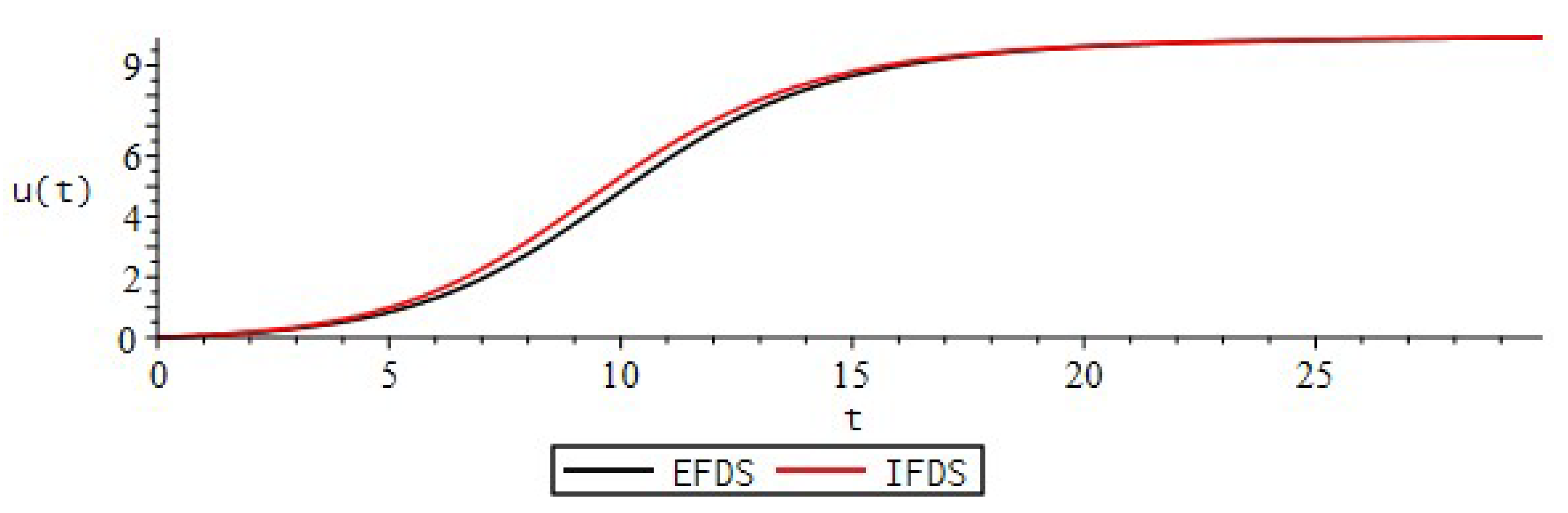
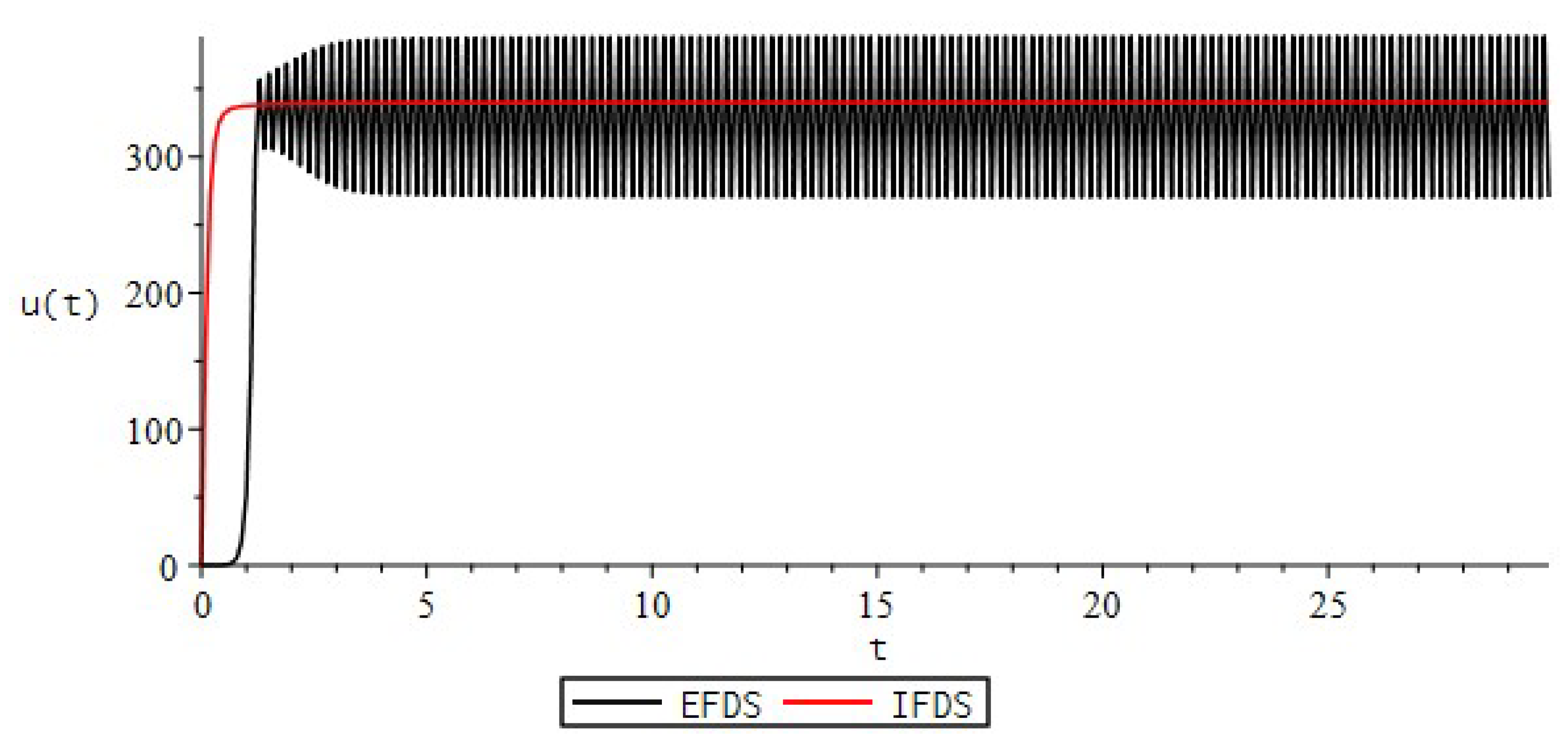
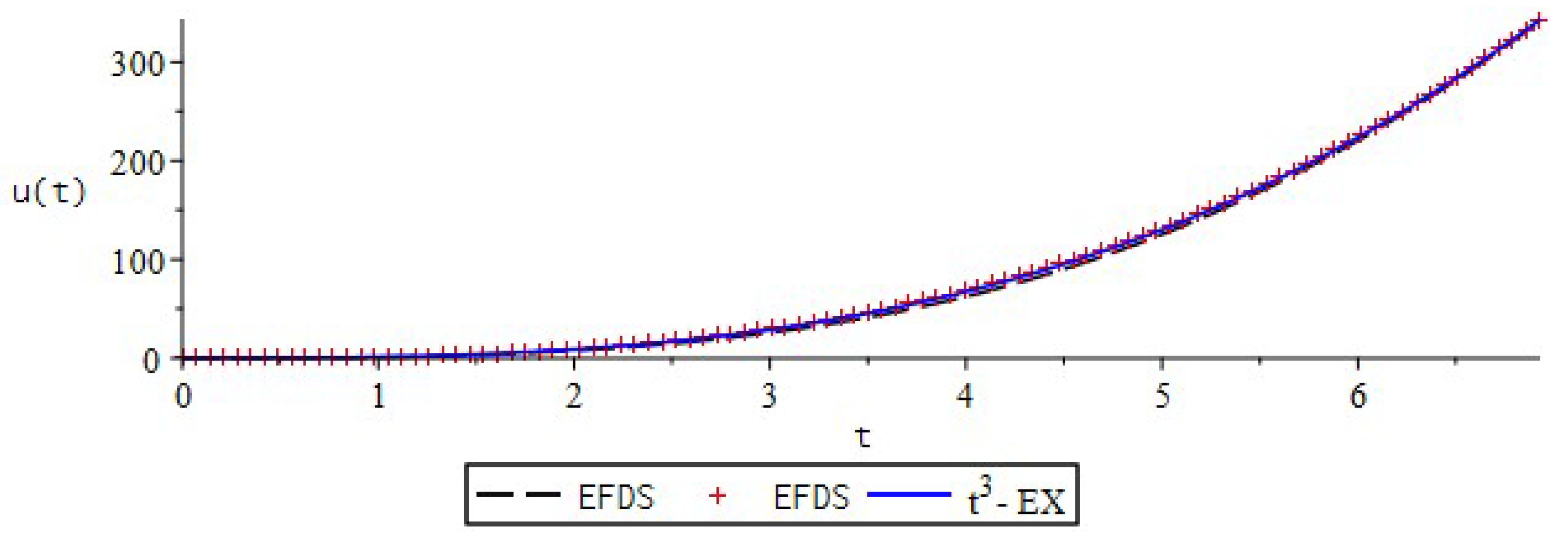
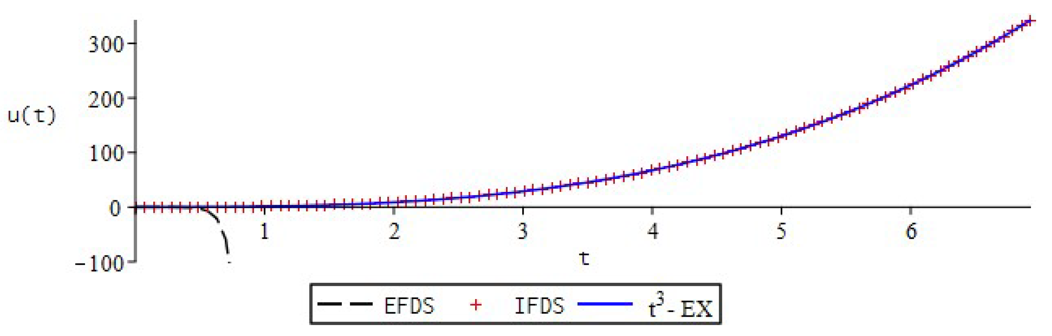
10. Computational Accuracy and Test Cases

Let us consider some examples: a non-local implicit finite-difference scheme (IFDS) (32) resolved by the modified Newton’s method (MNM) (34), as well as an explicit finite-difference scheme (EFDS) (38), which were implemented in the Maple 2021 computer mathematics environment.

Example 1.

Consider the case when $a\left(t\right),b\left(t\right),c\left(t\right)$ and $\alpha \left(t\right)$ are constants: $b=0.5,a=c=0.05$ and $\alpha =0.9$. The rest of the parameters are taken as follows: $u\left(0\right)=0,N=100,T=30$. Indeed, for such values of the parameters, the condition from Theorem 5 is satisfied: $\tau <\frac{2^{1-\widehat{\alpha }}-1}{\overline{b}}$ performed: $0.1<0.143$. Then, by (IFDS) (32) and EFDS (38) we get the calculated curves of the Figure 1. Data can be seen from supplementary material.

From Figure 1, it can be seen that the calculated curve has an s-shape, which is typical for dynamic processes in saturated media. It can also be seen that the trend of the calculated curves is increasing with the exit to the steady state. As the value of the b parameter increases and the value of the a parameter decreases, the s-shape becomes more pronounced.

Let us evaluate the computational accuracy of EFDS and IFDS.To do this, calculate the maximum error $\xi$ according to Runge’s rule, that is, ${\displaystyle \xi =\underset{\begin{array}{c}i\end{array}}{max}\left(\frac{|u_i-u_{2i}|}{2^{p_{Aprior}}-1}\right)}$, where $u_i$ and $u_{2i}$—calculated values obtained by formulas (32) and (38) on step $\tau$ and $\tau /2$ respectively, $p_{Aprior}=2-\alpha$—theoretical order of convergence for IFDS, $p_{Aprior}=1$—for EFDS. The computational accuracy is determined by the formula: $p={log}_2({\xi }_i/{\xi }_{i+1})$.

From

Table 1. Computational accuracy of EFDS and IFDS, at $T=30$.

			EFDS		IFDS
i	N	$\mathbf{\tau }$	$\mathbf{\xi }$	$\mathit{p}$	$\mathbf{\xi }$	$\mathit{p}$
1	20	3/2	3.84086	-	2.17611	-
2	40	3/4	2.25311	0.76951	1.10581	0.97664
3	80	3/8	1.21857	0.88671	0.48416	1.19153
4	160	3/16	0.64976	0.90720	0.22022	1.13650
5	320	3/32	0.34048	0.93231	0.10018	1.13630
6	640	3/64	0.17676	0.94577	0.04548	1.13917
7	1280	3/128	0.09126	0.95368	0.02056	1.14522

it can be seen that, with an increase in the nodes of the computational grid, the maximum error decreases and the computational accuracy for EFDS tends to unity, which corresponds to the condition of Theorem 5, and for IFDS it tends to the theoretical one according to (15 ) Lemma 3.

It should also be noted that the IFDS scheme has better accuracy, and the maximum error is an order of magnitude less than that of the EFDS.

Consider also for this example the case when the condition from Theorem 5: $\tau <\frac{2^{1-\widehat{\alpha }}-1}{\overline{b}}$ is violated. To do this, it is enough to take the values of b an order of magnitude larger, for example, $b=17$ then: $0.1>0.004$, and we leave the values of other parameters unchanged. Design curves: for EFDS obtained by the formula (38), and for IFDS by the formula (32), are shown in Figure 2.

Example 2.

Using the property of the fractional integral, we show that by solving the Cauchy problem:

$${\partial }_{0t}^{\alpha \left(t\right)}u\left(\tau \right)+a\left(t\right)u^2\left(t\right)-b\left(t\right)u\left(t\right)-c\left(t\right)=0,u\left(0\right)=u_0=0,$$

is the function $u\left(t\right)=t^3$. Indeed, according to the work [48] with:

$${\partial }_{0t}^{\alpha \left(t\right)}{t}^3=\frac{1}{\mathsf{\Gamma }(1-\alpha (t\left)\right)}{\int }_0^t\frac{{\left({\tau }^3\right)}^{\prime }d\tau }{{(t-\tau )}^{\alpha \left(t\right)}}=\frac{3}{\mathsf{\Gamma }(1-\alpha (t\left)\right)}{\int }_0^t\frac{{\tau }^{2}d\tau }{{(t-\tau )}^{\alpha \left(t\right)}}=\frac{3\mathsf{\Gamma }\left(3\right)t^{3-\alpha \left(t\right)}}{\mathsf{\Gamma }(4-\alpha (t\left)\right)},$$

we get that:

$$\begin{array}{c}\hfill \begin{array}{c}{\partial }_{0t}^{\alpha \left(t\right)}u\left(\tau \right)+a\left(t\right)u^2\left(t\right)-b\left(t\right)u\left(t\right)-c\left(t\right)=0,u\left(0\right)=u_0=0,\\ c\left(t\right)=\frac{3\mathsf{\Gamma }\left(3\right)t^{3-\alpha \left(t\right)}}{\mathsf{\Gamma }(4-\alpha (t\left)\right)}+a\left(t\right)u^6\left(t\right)-b\left(t\right)u^3\left(t\right).\end{array}\end{array}$$

(43)

Notice that $\alpha \left(t\right)=\alpha \left(t_k\right)=const$, which means for the EFDS schema (38) $\alpha \left(t\right)=\alpha \left(t_{k+1}\right)=const$.

Consider (43), with parameters similar to example 1, when: $c\left(t\right)=\frac{3\mathsf{\Gamma }\left(3\right)t^{3-\alpha \left(t\right)}}{\mathsf{\Gamma }(4-\alpha (t\left)\right)}+a\left(t\right)u^6\left(t\right)-b\left(t\right)u^3\left(t\right)$, $b=0.7$, $a=0.005$ and $\alpha =0.8$. Other parameters: $u\left(0\right)=0,N=100,T=7$. Condition from Theorem 5: $\tau <\frac{2^{1-\widehat{\alpha }}-1}{\overline{b}}$ executed: $0.07<0.2124$. The calculated curves are shown in Figure 3.

Let us estimate the computational accuracy: the exact solution EX: $u\left(t\right)=t^3$, IFDS and EFDS. To do this, we calculate the maximum error $\xi$ between the obtained solutions, that is, $\xi ={max}_{\begin{array}{c}i\end{array}}\left(|u_{i,M1}-u_{i,M2}|\right)$, where $u_{i,M1}$ and $u_{i,M2}$—calculated values obtained by one and the second method, respectively.

From

Table 2. Computational precision: accurate solution EX, EFDS and IFDS, at $T=1$.

			EX – EFDS		EX – IFDS
i	N	$\mathbf{\tau }$	$\mathbf{\xi }$	$\mathit{p}$	$\mathbf{\xi }$	$\mathit{p}$
1	20	1/20	0.14430	-	0.05206	-
2	40	1/40	0.07790	0.88928	0.02274	1.19515
3	80	1/80	0.04112	0.92166	0.00993	1.19410
4	160	1/160	0.02140	0.94215	0.00434	1.19527
5	320	1/320	0.01103	0.95550	0.00189	1.19671
6	640	1/640	0.00565	0.96457	0.00082	1.19788
7	1280	1/1280	0.00288	0.97105	0.00035	1.19870

, as we can see, for EFDS and IFDS schemes, in comparison with the exact EX solution, with an increase in the nodes of the computational grid, the maximum error $\xi$ decreases, and for IFDS the error value is an order of magnitude less. Computational accuracy p for EFDS tends to unity, which corresponds to the condition of Theorem 5, and for IFDS, tends to theoretical $p_{Aprior}=2-\alpha$ according to (15) Lemma 3.

Similarly to Example 1, consider the case when the condition from Theorem 5: $\tau <\frac{2^{1-\widehat{\alpha }}-1}{\overline{b}}$ is violated. We take b an order of magnitude more, $b=18$ then: $0.07>0.008$, and we leave the values of other parameters unchanged. The calculated curves are shown in Figure 4.

From Figure 4, we see that the EFDS scheme (38) falls apart when the condition $\tau <\frac{2^{1-\widehat{\alpha }}-1}{\overline{b}}$ is violated, similar to the case from example 1.

Example 3.

Consider the case when in the model fractional Riccati Equation (31) the variable order of fractionality: $\alpha \left(t\right)=0.9-0.1t/T$ is a monotonically decreasing function, equation coefficients: $a\left(t\right)={cos}^2\left(t\right)/T$, $b\left(t\right)=1-0.1t/T$, $c\left(t\right)={sin}^2\left(t\right)/T$, and the rest of the parameters: $u\left(0\right)=0.9,N=2000,T=20$. Condition: $\tau <\frac{2^{1-\widehat{\alpha }}-1}{\overline{b}}$ performed for EFDS: $0.01<0.07$. Modeling results using formulasIFDS (32) and EFDS (38) give the calculated curves in Figure 5.

The calculated curves in Figure 5 obtained by the numerical methods IFDS and EFDS practically coincided. Due to the fact that the coefficients in the model Equation (31) change according to the harmonic law, their shape resembles the shape of curves for oscillatory processes. We also note that the general trend of the calculated curves is an increasing one when the steady-state regime is reached. Similar dynamics are found in economics when describing cycles and crises [49].

Let us evaluate the computational accuracy of EFDS and IFDS, similar to Example 1.

For the case of $\alpha \left(t\right)$ and $a\left(t\right),b\left(t\right),c\left(t\right)$—functions, we see from

Table 3. Computational accuracy EFDS and IFDS, at $T=10$.

			EFDS		IFDS
i	N	$\mathbf{\tau }$	$\mathbf{\xi }$	$\mathit{p}$	$\mathbf{\xi }$	$\mathit{p}$
1	20	1/2	16.9716	-	21.8875	-
2	40	1/4	4.10786	2.04666	5.21343	2.06980
3	80	1/8	2.83581	0.53462	2.14741	1.27963
4	160	1/16	1.70580	0.73330	0.90911	1.24006
5	320	1/32	0.95277	0.84024	0.39496	1.20272
6	640	1/64	0.51645	0.88350	0.17357	1.18613
7	1280	1/128	0.27275	0.92105	0.07673	1.17768

that, with an increase in the nodes of the computational grid, the maximum error $\xi$ decreases, and for IFDS the error value is an order of magnitude less. Computational accuracy p for EFDS tends to unity, which corresponds to the condition of Theorem 5, and for IFDS, tends to theoretical ${\displaystyle p_{Aprior}=2-\underset{t}{max}\left(\alpha \left(t\right)\right)=2-0.9=1.1}$ according to (15) Lemma 3.

Example 4.

Consider the case when, in the model fractional Riccati Equation (31), the variable order of fractionality: $\alpha \left(t\right)=0.4+0.5t/T$ is a monotonically increasing function, the coefficients of the equation are: $a\left(t\right)={cos}^2\left(t\right)/T$, $b\left(t\right)=1-0.1t/T$, $c\left(t\right)={sin}^2\left(t\right)/T$, and the remaining parameters: $u\left(0\right)=0.9,N=2000,T=20$. Condition: $\tau <\frac{2^{1-\widehat{\alpha }}-1}{\overline{b}}$ performed for EFDS: $0.01<0.07$. Modeling results using formulas IFDS (32) and EFDS (38) give the calculated curves in Figure 6.

Let us evaluate the computational accuracy of EFDS and IFDS, similar to Example 3.

We see from

Table 4. Computational accuracy EFDS and IFDS, at $T=10$.

			EFDS		IFDS
i	N	$\mathbf{\tau }$	$\mathbf{\xi }$	$\mathit{p}$	$\mathbf{\xi }$	$\mathit{p}$
1	20	1/2	4.62978	-	18.3955	-
2	40	1/4	3.95342	0.22784	4.11895	2.15900
3	80	1/8	3.04877	0.37487	1.65080	1.31910
4	160	1/16	1.93859	0.65321	0.66586	1.30986
5	320	1/32	1.16042	0.74036	0.27601	1.27050
6	640	1/64	0.64893	0.83850	0.11415	1.27376
7	1280	1/128	0.34560	0.90893	0.04734	1.26961

that, with an increase in the nodes of the computational grid, the maximum error $\xi$ decreases, and for IFDS the error value is an order less. Computational accuracy p for EFDS tends to unity, which corresponds to the condition of Theorem 5, and for IFDS, tends to theoretical ${\displaystyle p_{Aprior}=2-\underset{t}{max}\left(\alpha \left(t\right)\right)=2-0.9=1.1}$ according to (15) Lemma 3.

Example 5.

Consider the case when, in the model fractional Riccati Equation (31), the variable order of fractionality: $\alpha \left(t\right)=0.4+{sin}^2\left(t\right)/2$ is a periodic function, the coefficients of the equation are: $a\left(t\right)={cos}^2\left(t\right)/T$, $b\left(t\right)=1-0.1t/T$, $c\left(t\right)={sin}^2\left(t\right)/T$, and the remaining parameters: $u\left(0\right)=0.9,N=2000,T=20$. Condition: $\tau <\frac{2^{1-\widehat{\alpha }}-1}{\overline{b}}$ performed for EFDS: $0.01<0.07$. Modeling results using formulas IFDS (32) and EFDS (38) give the calculated curves in Figure 7.

Let us evaluate the computational accuracy of EFDS and IFDS, similar to Examples 3 and 4.

We see from

Table 5. Computational accuracy EFDS and IFDS, at $T=10$.

			EFDS		IFDS
i	N	$\mathbf{\tau }$	$\mathbf{\xi }$	$\mathit{p}$	$\mathbf{\xi }$	$\mathit{p}$
1	20	1/2	4.53506	-	23.0946	-
2	40	1/4	3.23887	0.48562	4.58889	2.33133
3	80	1/8	2.65104	0.28893	1.64571	1.47942
4	160	1/16	1.71817	0.62568	0.64363	1.35441
5	320	1/32	1.01576	0.75831	0.26495	1.28046
6	640	1/64	0.56034	0.85818	0.11185	1.24414
7	1280	1/128	0.29775	0.91215	0.04785	1.22502

that, with an increase in the nodes of the computational grid, the maximum error $\xi$ decreases, and for IFDS the error value is an order less. Computational accuracy p for EFDS tends to unity, which corresponds to the condition of Theorem 5, and for IFDS, tends to theoretical ${\displaystyle p_{Aprior}=2-\underset{t}{max}\left(\alpha \left(t\right)\right)=2-0.9=1.1}$ according to (15) Lemma 3.

11. Software Package for Maple 2021 Environment

The library <<FDREext>> (short for Fractional Derivative in Riccati Equation Extended) otherwise (<<FDRE>> version 2.0) was developed as part of the software package for solving problems of numerical modeling using the Riccati equation with the Gerasimov-Caputo fractional differentiation operator. The software package is implemented in the environment of symbolic computer mathematics Maple 2021, and is a development and generalization of the previously developed programs <<NSFDRE>> version 1.0 implemented in C ++, and the program <<FDRE>> version 1.0 in Maple language.

The main difference between the developed new software package from the previous one is the ability to use the wide functionality of the Maple 2021 environment, which is reflected in the following:

• implementation of a non-local explicit finite difference scheme (EFDS);
• implementation of a non-local implicit finite difference scheme (IFDS);
• implementation of the modified Newton’s method (MNM), for solving the IFDS scheme;
• implementation of modifications of the Gerasimov-Caputo fractional operator of the form $\alpha (t-\tau )$ and $\alpha \left(\tau \right)$, considered in [50];
• the ability to set the coefficients $a\left(t\right),b\left(t\right),c\left(t\right)$ of functions from t;
• the ability to set non-constant $\alpha \left(t\right)$ as a function of t.

The basis of the developed library (module) <<FDREext>> is: the module (function) $ApproxFractDeriv\left(\right)$—which implements numerical methods for solving the fractional Riccati equation with a derivative in the sense of Gerasimov-Caputo.

A number of auxiliary figures are also implemented. Figure 8 procedures (functions) for:

• $ClearSeq\left(\right)$—clears the transmitted data from the specified elements;
• $CreateFileName\left(\right)$—create a name for a custom file;
• $CreateFilePath\left(\right)$—display the path to the $.mw$ file where the function is called;
• $ExcelExtractColumn\left(\right)$—extract a column from a $.xlsx$ file;
• $ExtendedData\left(\right)$—cubic spline data smoothing;
• $NormalizeOnMax\left(\right)$—normalization of the transmitted data to the maximum;
• $PeriodicFunc\left(\right)$—periodic function $0<x<1$;
• $PlotData\left(\right)$—displaying the chart based on the transmitted data;
• $ResearchOnError\left(\right)$—investigation of the solution for computational accuracy and maximum error;
• $TextExtractColumn\left(\right)$—extract a column from a $.txt$ file;
• $WriteFile\_txt\left(\right)$—output the results to a $.txt$ file;
• $WriteFile\_xlxs\left(\right)$—output the results to a $.xlsx$ file.

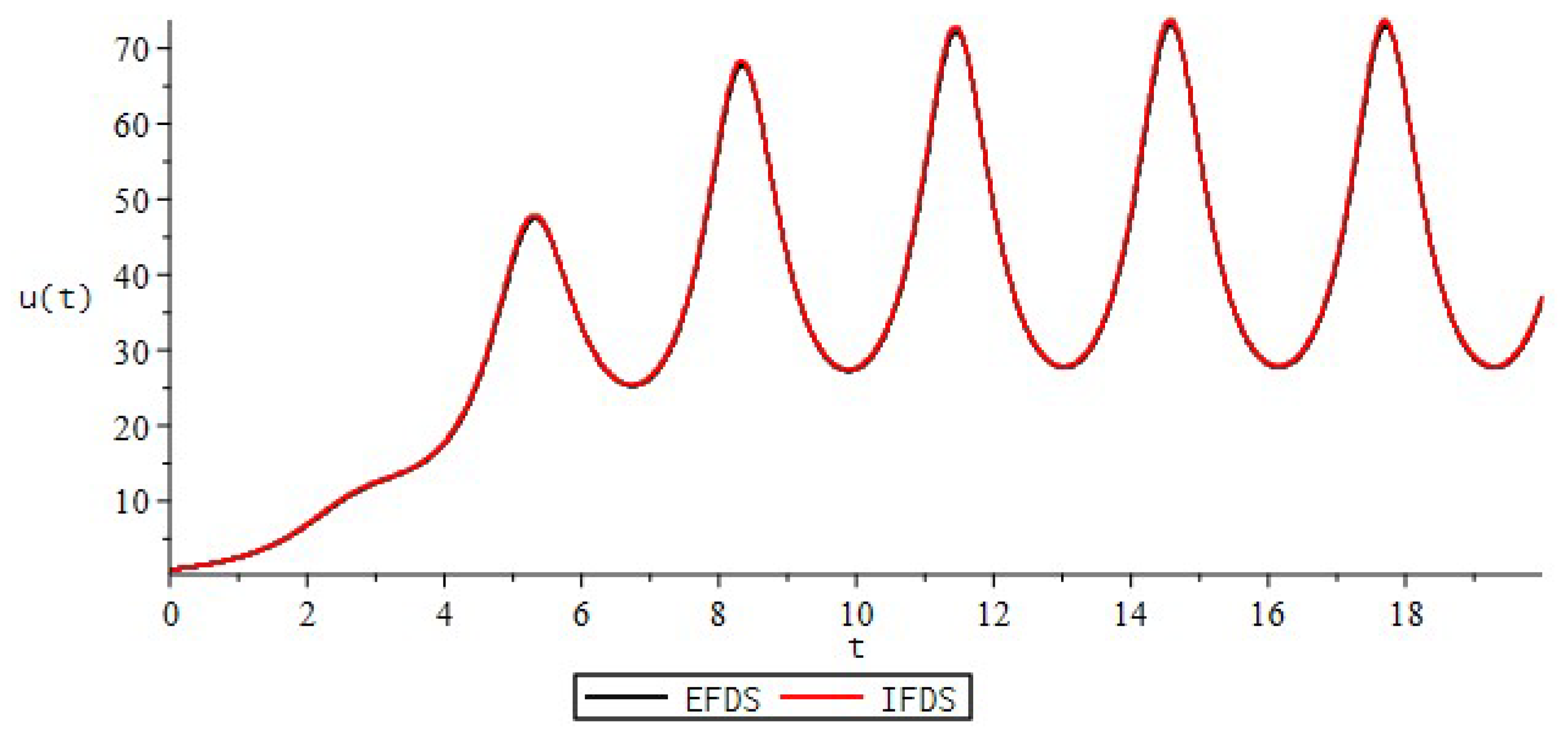
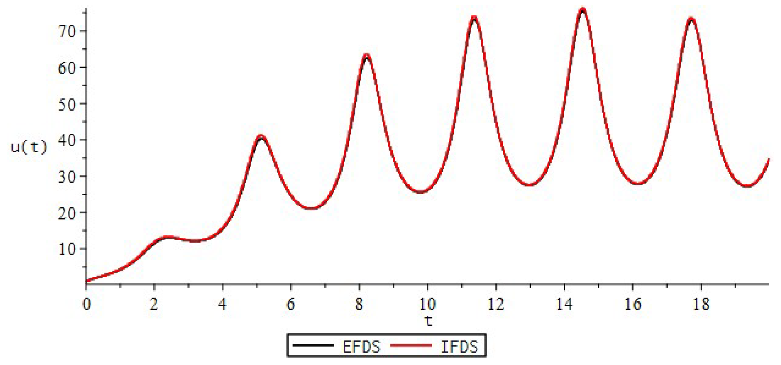
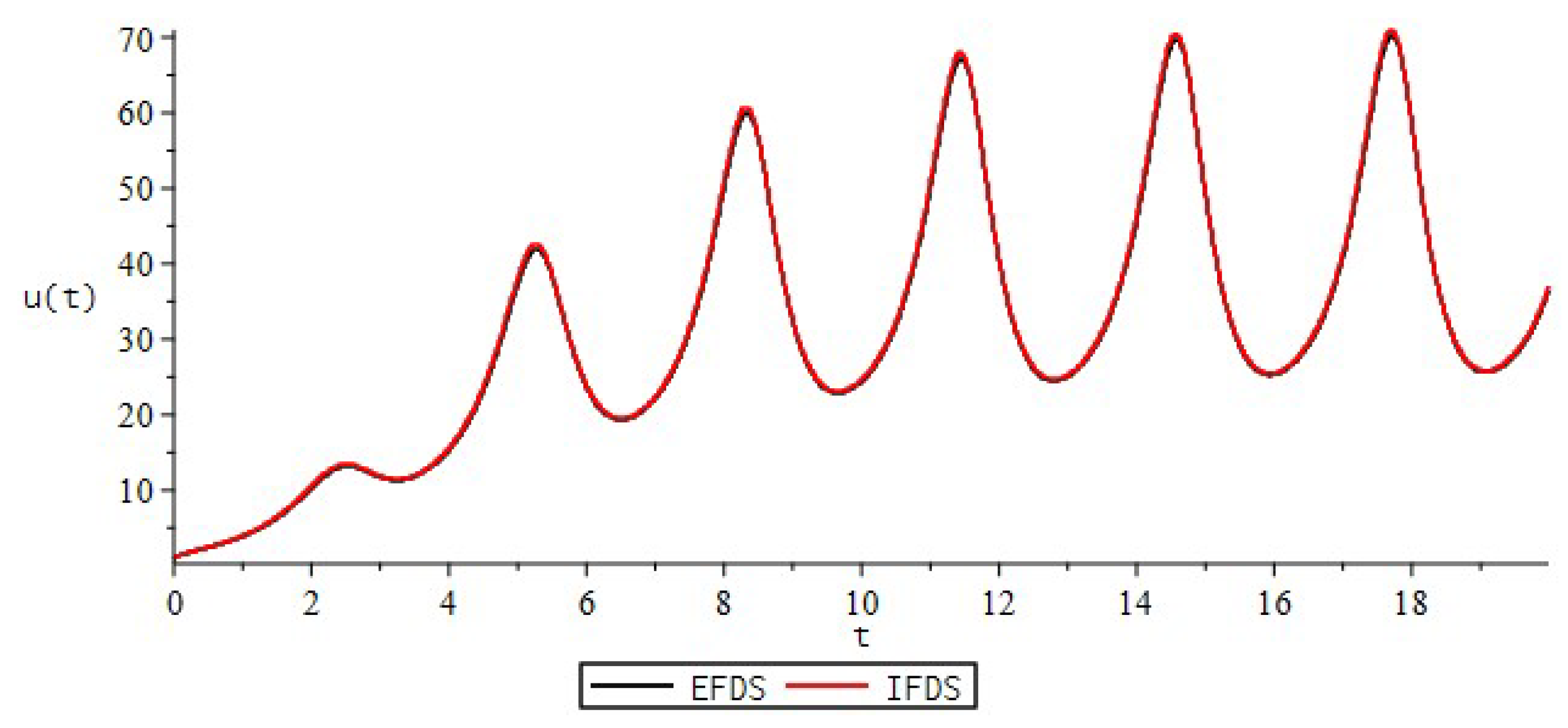
12. Some Applications of the Fractional Riccati Equation

Various applications of the fractional Riccati equation for modeling dynamic processes with saturation are considered: the dynamics of solar activity [51], the dynamics of radon accumulation in the storage chamber [52] and the dynamics of the spread of coronavirus infection Covid-19 in the Republic of Uzbekistan and the Russian Federation [53].

Using the experimental data of the processes described above, the parameters of the proposed mathematical model were best determined, based on the fractional Riccati equation with non-constant coefficients and the derivative of the fractional variable order of the Gerasimov-Caputo type, which indicates its adequacy and applicability to saturation processes taking into account dynamic memory.

It is shown that with an optimal choice of the corresponding simulation parameters: $\alpha \left(t\right)$ and $a\left(t\right),b\left(t\right),c\left(t\right)$, the calculated curves are in good agreement with the experimental data. The model (31), when choosing the appropriate parameters, can also provide some forecasts about the possible investigation of the processes under consideration.

Further continuation of the work associated with applications of the developed mathematical model may consist in the refinement of the model parameters as a result of solving the corresponding inverse problem, as well as in their further understanding.

13. Conclusions

The main contributions of this research are as follows:

• A mathematical model is proposed for describing processes with saturation based on the fractional Riccati equation with variable coefficients and the derivative of a fractional variable order of the Gerasimov-Caputo type;
• Numerical methods for solving the Cauchy problem for a mathematical model are proposed: non-local EFDS, non-local IFDS, and also MNM for solving IFDS;
• The questions of approximation, stability and convergence of methods are investigated. It is shown that the EFDS converge conditionally with the first order of accuracy $O\left(\tau \right)$. IFDS is stable and has convergence order $O\left({\tau }^{2-\widehat{\alpha }}\right)$;
• This theoretical result is confirmed by specific test examples and estimates of the computational accuracy according to Runge’s rule. It is important to note that, as a test case, the case of comparing a numerical solution using the IFDS and EFDS schemes with an exact solution is also considered. It is shown that the order of computational accuracy of numerical methods approaches the theoretical order of accuracy with an increase in the nodes of the computational grid;
• A library in the environment of symbolic mathematics Maple 2021 has been developed, which contains procedures for the numerical analysis of the fractional Riccati equation with a variable fractional order derivative of the Gerasimov-Caputo type and non-constant coefficients with the ability to visualize the simulation results.

Further continuation of the work, connected with the theoretical issues of the developed mathematical model, may consist, for example, in investigating the behavior of a numerical solution and its stability under the influence of random noise.

14. Patents

Algorithms that implement calculations according to: numerical methods, processing of results, comparison with experimental data and visualization are implemented in the author’s library <<FDREext>> (short for Fractional Derivative in Riccati Equation Extended) otherwise (<<FDRE>> versions 2.0) for the environment of symbolic computer mathematics Maple 2021. A certificate of state registration of computer programs was obtained for the developed library.

References

1. Nazarov, V.E.; Kiyashko, S.B. Wave processes in media with inelastic hysteresis with saturation of nonlinear losses. Radiophysics 2016, 59, 124–136. (In Russian) [Google Scholar]
2. Kurkin, A.A.; Kurkina, O.E.; Pelenovskij, E.N. Logistic models for the spread of epidemics. Proc. NSTU Im. R.E. Alekseeva 2020, 129, 9–18. (In Russian) [Google Scholar]
3. Volterra, V. Theory of Functionals and of Integral and Integro-Differential Equations; Dover Publications: Mineola, NY, USA, 2005; p. 288. [Google Scholar]
4. Volterra, V. Sur les ´equations int´egro-differentielles et leurs applications. Acta Math. 1912, 35, 295–356. [Google Scholar] [CrossRef]
5. Uchajkin, V.V. Fractional Derivatives Method; Artichoke: Ulyanovsk, Russia, 2008; p. 510. (In Russian) [Google Scholar]
6. Nakhushev, A.M. Fractional Calculus and Its Applications; Fizmatlit: Moscow, Russia, 2003; p. 272. (In Russian) [Google Scholar]
7. Ortigueira, M.D.; Machado, J.T. What is a fractional derivative? J. Comput. Phys. 2015, 321, 4–13. [Google Scholar] [CrossRef]
8. Kilbas, A.A.; Srivastava, H.M.; Trujillo, J.J. Theory and Applications of Fractional Differential Equations; Elsevier Science Limited: Amsterdam, The Netherland, 2006; Volume 204, p. 523. [Google Scholar]
9. Uchaikin, V.V. Fractional Derivatives for Physicists and Engineers; Vol. I. Background and Theory; Springer: Berlin/Heidelberg, Germany, 2013; p. 373. [Google Scholar]
10. Ortigueira, M.D.; Valerio, D.; Machado, J.T. Variable order fractional systems. In Communications in Nonlinear Science and Numerical Simulation; Elsevier: Amsterdam, The Netherland, 2019; Volume 71, pp. 231–243. [Google Scholar] [CrossRef]
11. Parovik, R.I. Mathematical Modeling of Linear Hereditary Oscillators; Kamchatka State University Named after Vitus Bering: Petropavlovsk-Kamchatsky, Russia, 2015; p. 187. (In Russian) [Google Scholar]
12. Pskhu, A.V. Uravneniya v Chastnyh Proizvodnyh Drobnogo Poryadka; Science: Moscow, Russia, 2005; p. 199. (In Russian) [Google Scholar]
13. Mamchuev, M.O. Boundary Value Problems for Equations and Systems of Partial Differential Equations of Fractional Order; Publishing House KBSC RAS: Nalchik, Russia, 2015; p. 200, (In Russian). [Google Scholar] [CrossRef]
14. Shogenov, V.K.; Akhkubekov, A.A.; Akhkubekov, R.A. Fractional differentiation method in the theory of Brownian motion. Izv Vyssh. Uchebn. Zaved. Severo-Kavkaz. Reg. Estestv. Nauki. 2004, 1, 46–50. [Google Scholar]
15. Méhauté, A.L.; Nigmatullin, R.R.; Nivanen, L. Flèches du Temps et Géométrie Fractale; Hermes: Paris, France, 1998; p. 348. [Google Scholar]
16. Kobelev, Y.L. Phenomenological Models for Describing Large Systems with Fractal Structures. In Abstract of the Dissertation of the Candidate of Physical and Mathematical Sciences; Ural State University A.M. Gorky: Yekaterinburg, Russia, 2001. (In Russian) [Google Scholar]
17. Sun, H.; Chen, W.; Wei, H.; Chen, Y.Q. A comparative study of constant-order and variable-order fractional models in characterizing memory property of systems. Eur. Phys. J.-Spec. Top. 2011, 193, 185–192. [Google Scholar] [CrossRef]
18. Sun, H.; Chen, W.; Li, C.; Chen, Y. Finite difference schemes for variable-order time fractional diffusion equation. Int. J. Bifurc. Chaos 2012, 22, 1250085. [Google Scholar] [CrossRef] [Green Version]
19. Momani, S.; Shawagfeh, N. Decomposition method for solving fractional Riccati differential equations. Appl. Math. Comput. 2006, 182, 1083–1092. [Google Scholar] [CrossRef]
20. Tan, Y.; Abbasbandy, S. Homotopy analysis method for quadratic Riccati differential equation. Commun. Nonlinear Sci. Numer. Simul. 2008, 13, 539–546. [Google Scholar] [CrossRef]
21. Jafari, H.; Tajadodi, H. He’s variational iteration method for solving fractional Riccati differential equation. Int. J. Differ. Equ. 2010, 2010, 1–8. [Google Scholar] [CrossRef] [Green Version]
22. Khan, N.A.; Ara, A.; Jamil, M. An efficient approach for solving the Riccati equation with fractional orders. Comput. Math. Appl. 2011, 61, 2683–2689. [Google Scholar] [CrossRef] [Green Version]
23. Sweilam, N.H.; Khader, M.M.; Mahdy, A.M.S. Numerical studies for solving fractional Riccati differential equation. Appl. Appl. Math. 2012, 7, 595–608. [Google Scholar]
24. Merdan, M. On the solutions fractional Riccati differential equation with modified Riemann–Liouville derivative. Int. J. Differ. Equ. 2012, 2012, 1–17. [Google Scholar] [CrossRef]
25. Khader, M.M. Numerical treatment for solving fractional Riccati differential equation. J. Egypt. Math. Soc. 2013, 21, 32–37. [Google Scholar] [CrossRef] [Green Version]
26. Khader, M.M.; Mahdy, A.M.S.; Mohamed, E.S. On approximate solutions for fractional Riccati differential equation. Int. J. Eng. Appl. Sci. 2014, 4, 1–10. Available online: https://citeseerx.ist.psu.edu/viewdoc/download?doi=10.1.1.682.4526&rep=rep1&type=pdf (accessed on 15 November 2021).
27. Ezz-Eldien, S.S. On solving fractional logistic population models with applications. Comput. Appl. Math. 2018, 37, 6392–6409. [Google Scholar] [CrossRef]
28. Khan, N.A.; Ara, A.; Khan, N.A. Fractional-order Riccati differential equation: analytical approximation and numerical results. Adv. Differ. Equ. 2013, 185. [Google Scholar] [CrossRef] [Green Version]
29. Salehi, Y.; Darvishi, M.T. An investigation of fractional Riccati differential equation. Int. J. Light Electron Opt. 2016, 127, 11505–11521. [Google Scholar] [CrossRef]
30. Aminikhah, H.; Sheikhani, A.H.R.; Rezazadeh, H. Approximate analytical solutions of distributed order fractional Riccati differential equation. Ain Shams Eng. J. 2018, 9, 581–588. [Google Scholar] [CrossRef] [Green Version]
31. Syam, M.I.; Alsuwaidi, A.; Alneyadi, A.; Al Refai, S.; Al Khaldi, S. Implicit hybrid methods for solving fractional Riccati equation. J. Nonlinear Sci. Appl. 2019, 12, 124–134. [Google Scholar] [CrossRef] [Green Version]
32. Khader, M.M.; Sweilam, N.H.; Kharrat, B.N. Numerical Simulation for Solving Fractional Riccati and Logistic Differential Equations as a Difference Equation. Appl. Appl. Math. Int. J. 2020, 15, 37. Available online: https://digitalcommons.pvamu.edu/aam/vol15/iss1/37/ (accessed on 21 December 2021).
33. Cai, M.; Li, C. Numerical approaches to fractional integrals and derivatives: A review. Mathematics 2020, 8, 43. [Google Scholar] [CrossRef] [Green Version]
34. Volterra, V. Mathematical Theory of the Struggle for Existence; Nauka: Moscow, Russia, 1976; p. 286. [Google Scholar]
35. Gerasimov, A.N. Generalization of linear deformation laws and their application to internal friction problems. AS USSR. Appl. Math. Mech. 1948, 12, 529–539. [Google Scholar]
36. Caputo, M. Linear models of dissipation whose Q is almost frequency independent—II. Geophys. J. Int. 1967, 13, 529–539. [Google Scholar] [CrossRef]
37. Caputo, M. Elasticita e Dissipazione; Zanichelli: Bologna, Italy, 1969; p. 150. [Google Scholar]
38. Oldham, K.; Spanier, J. The Fractional Calculus Theory and Applications of Differentiation and Integration to Arbitrary Order; Academic Press: London, UK, 1974; p. 240. [Google Scholar]
39. Parovik, R.I. Mathematical models of oscillators with memory. Oscil.-Recent Dev. 2019, 3–21. [Google Scholar] [CrossRef] [Green Version]
40. Parovik, R.I. On a finite-difference scheme for an hereditary oscillatory equation. J. Math. Sci. 2021, 253, 547–557. [Google Scholar] [CrossRef]
41. Parovik, R.I. Explicit finite-difference scheme for the numerical solution of the model equation of nonlinear hereditary oscillator with variable-order fractional derivatives. Arch. Control. Sci. 2016, 26, 429–435. [Google Scholar] [CrossRef] [Green Version]
42. Parovik, R.I. Mathematical modeling of linear fractional oscillators. Math. Model. Linear Fract. Oscil. 2020, 8, 1879. [Google Scholar] [CrossRef]
43. Parovik, R.I.; Tverdyi, D.A. Some Aspects of Numerical Analysis for a Model Nonlinear Fractional Variable Order Equation. Math. Comput. Appl. 2021, 26, 55. [Google Scholar] [CrossRef]
44. Cai, M.; Li, C. Theory and Numerical Approximations of Fractional Integrals and Derivatives; Society for Industrial and Applied Mathematics: Philadelphia, PA, USA, 2020; p. 317. [Google Scholar] [CrossRef] [Green Version]
45. Torres-Hernandez, A.; Brambila-Paz, F.; Iturrarán-Viveros, U.; Caballero-Cruz, R. Fractional Newton–Raphson Method Accelerated with Aitken’s Method. Axioms 2021, 10, 47. [Google Scholar] [CrossRef]
46. Tvyordyj, D.A. Hereditary Riccati equation with fractional derivative of variable order. J. Math. Sci. 2021, 253, 564–572. [Google Scholar] [CrossRef]
47. Garrappa, R. Numerical Solution of Fractional Differential Equations: A Survey and a Software Tutorial. Mathematics 2018, 6, 16. [Google Scholar] [CrossRef] [Green Version]
48. Tverdyi, D.A. Investigation of numerical methods for solving the Riccati equation with a fractional derivative of variable order. Probl. Comput. Appl. Math. 2021, 23, 5–18. (In Russian) [Google Scholar]
49. Korotayev, A.V.; Grinin, L.E. Kondratieff waves in the world system perspective. In Kondratieff Waves. Dimensions and Prospects at the Dawn of the 21st Century; Uchitel: Volgograd, Russia, 2012; pp. 23–64. [Google Scholar]
50. Tverdyi, D.A.; Parovik, R.I. Research of the Hereditary Dynamic Riccati System with Modification Fractional Differential Operator of Gerasimov-Caputo. AIP Conf. Proc. 2021, 2365, 020011. [Google Scholar] [CrossRef]
51. Tverdyi, D.A.; Parovik, R.I. Mathematical modeling of the dynamics of solar activity using the fractional Riccati equation with variable heredity. In Proceedings of the VI International Scientific Conference IAMA KBSC RAS, Nalchik, Russia, 5–9 December 2021; p. 155. (In Russian). [Google Scholar]
52. Tverdyi, D.A.; Parovik, R.I.; Makarov, E.O.; Firstov, P.P. Application of the Riccati hereditary mathematical model to the study of the dynamics of radon accumulation in the storage chamber. In EPJ Web of Conferences; EDP Sciences: Paris, France, 2021; Volume 254, pp. 1–5. [Google Scholar] [CrossRef]
53. Tverdyi, D.A.; Parovik, R.I. Fractional Riccati equation to model the dynamics of COVID-19 coronovirus infection. J. Physics Conf. Ser. 2021, 2094, 032042. [Google Scholar] [CrossRef]
Figure 1. Numerical solutions of the fractional Riccati equation with constant coefficients and α = 0.9 taking into account the fulfillment of the condition.
Fractalfract 06 00023 g001
Figure 2. Numerical solutions of the fractional Riccati equation with constant coefficients and α = 0.9 when the condition is violated.
Fractalfract 06 00023 g002
Figure 3. Exact solution EX: u ( t ) = t 3 and numerical solutions of the fractional Riccati equation with constant coefficients and α = 0.8 , taking into account the fulfillment of the condition.
Fractalfract 06 00023 g003
Figure 4. Exact solution EX and numerical solutions of the fractional Riccati equation with constant coefficients and α = 0.8 when the condition is violated.
Fractalfract 06 00023 g004
Figure 5. Numerical solutions of the fractional Riccati equation with variable coefficients α ( t ) = 0.9 0.1 t / T —monotonically decreasing function
Fractalfract 06 00023 g005
Figure 6. Numerical solutions of the fractional Riccati equation with variable coefficients α ( t ) = 0.4 + 0.5 t / T —monotonically increasing function.
Fractalfract 06 00023 g006
Figure 7. Numerical solutions of the fractional Riccati equation with variable coefficients α ( t ) = 0.4 + sin 2 ( t ) / 2 —periodic function.
Fractalfract 06 00023 g007
Figure 8. Library call <<FDREext>>.
Fractalfract 06 00023 g008